Two-speed phase dynamics in Si(111) (7$\times$7)-(1$\times$1) phase transition

Abstract

We propose a natural two-speed model for the phase dynamics of Si(111) 7$\times$7 phase transition to high temperature unreconstructed phase. We formulate the phase dynamics by using phase-field method and adaptive mesh refinement. Our simulated results show that a 7$\times$7 island decays with its shape kept unchanged, and its area decay rate is shown to be a constant increasing with its initial area. LEEM experiments concerned are explained, which confirms that the dimer chains and corner holes are broken first in the transition, and then the stacking fault is remedied slowly. This phase-field method is a reliable approach to phase dynamics of surface phase transitions.

Introduction It is well known that bulk terminated 1$\times$1 semiconductor surfaces usually are unstable against reconstruction at low temperatures and some of the reconstructed surface phases transit to the 1$\times$1 ones at high temperatures01 . Si surfaces are well studied because silicon plays the centering role in modern computer industry02 ; 03 ; 04 and potential silicon-based spintronics05 . The most important Si surface phase is the Si(111) 7$\times$7 reconstructed surface das . It is the ground state structure of Si(111) surface and transits to an unreconstructed 1$\times$1 structure above $T_{c}$=1125 Krr2 ; rr3 ; rr5 ; f0 ; f1 ; f3 ; f4 ; f5 ; f6 ; s1 . In situ scanning-tunneling-microscopy (STM) observationsrr2 ; rr3 , supported by Monte Carlo simulationstMC1 ; f4 , indicated that the stacking faulted triangle unit is the basic building block in forming the 7$\times$7 surface phase. The phase transition is believed to be of first orderl1 ; f1 ; f3 ; f4 ; f5 ; f6 ; l3 ; tMC1 , although earlier data implied a continuous phase transitions1 . It is of much interest to clarify the phase dynamics during the phase transition. Low-energy electron microscopy (LEEM) imaging is a powerful approach to experimentally measure time-dependent surface phasesl2 ; l3 ; l4 . Recent LEEM results showed that big 7$\times$7 islands always decay faster than small ones, with area decay rates increasing with their initial areasl3 . It seams like that the area decays have something like momentum. This phenomenon is very intriguing. It means that the phase transition dynamics and the microscopic processes meanwhile are very much complex, what we have known about them may be just a tip of the iceberg, and therefore much more investigation is in need.

Here we investigate the time-dependent phase dynamics during the phase transition of Si(111) 7$\times$7 islands to the unreconstructed high temperature phase. Through analyzing experimental results and the atomic structures of both surface phases, we propose a two-speed model for the phase dynamics. We formulate the phase dynamics using phase field method, famous for various growth and solidification issuespf1 ; pf2 ; pf2a ; pf3 ; pf4 ; g1 ; g2 , and adaptive mesh refinement techniquepfa . Our simulated results indicate that the dimer chains and corner holes are broken first in the phase transition, and then follows the slower remedying of the stacking fault. Our simulated images and linear area decays of 7$\times$7 islands are in agreement with the experimental results, which supports the two-speed model. This is a reliable approach to understand the phase dynamics of the Si(111) 7$\times$7 phase transition and other surface phase transitions.

Experimental clues The bulk terminated Si(111) 1$\times$1 surface and the dimers-adatoms-stacking-fault (DAS) model of Si(111) 7$\times$7 reconstructed surface phase are shown in Fig. 1 das ; 01 . This 1$\times$1 surface is not experimentally realized. The real experimental phase at high-temperature is a “1$\times$1” phase that is formed by covering the bulk terminated 1$\times$1 surface with 0.25 monolayer (ML) of fast-moving adatomsr4a ; r4b . The 7$\times$7$\rightarrow$“1$\times$1” phase transition needs extra 0.17 ML of adatoms because the former has 0.08 (4/49) ML more adatoms than the bulk terminated 1$\times$1 surface. On the experimental side, the appearing of the 7$\times$7 LEED pattern, or the seventh-order spots, means that the “1$\times$1”$\rightarrow$7$\times$7 transition happens, and on the other hand the absence of it means that the 7$\times$7 structure is destroyedr22 . The adatoms stay at T₄ sites above the second-layer atoms in the 7$\times$7 surface, and some of them moves to H₃ sites above the forth-layer atoms when the surface transits to the “1$\times$1” phaser21 . The movement of adatoms from T₄ sites to H₃ sites or vice versa is easy because it can be realized without breaking any bond. The formation of the dimer chains, corner holes, and stacking fault is considered essential to the 7$\times$7 reconstructionr13 . The presence of the LEEM image means that the key 7$\times$7 factors, the dimer chains and corner holes, still exist. Without the key factors, the 7$\times$7 phase is destroyed. The resultant region without dimer chains and corner holes, although still having stacking-fault, cannot be distinguished from the “1$\times$1” phase by means of LEEM experiment, being ‘ghost’ region to LEEM imagingr24 .

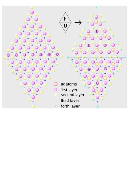
Figure 1: (color online). The atomic structures of bulk terminated Si(111) 1$\times$1 surface (left) and the DAS model of Si(111) 7$\times$7 reconstructed surface (right). The top four layers are shown for both structures, and in addition, the 12 adatoms are included for the latter. The 7$\times$7 unit is divided into the faulted (F, upper) half and the unfaulted (U, lower) half by the dash line.

Model and phase-field realization Therefore, we believe that the atoms reorganization during the 7$\times$7$\rightarrow$“1$\times$1” transition can be described by two basic processes: (a) the destroying of the dimer chains and corner holes, and (b) the remedying of the stacking-fault. The latter process should take more time because it requires collective movement of many atoms concerned. We adopt phase field methodpf1 ; pf2 ; pf2a ; pf3 ; pf4 to simulate the phase dynamics during the 7$\times$7$\rightarrow$“1$\times$1” transition. We use phase-field variables $\phi$ and $\xi$ together to describe the 7$\times$7 phase with respect to the “1$\times$1” phase. $\phi$ is used for the aspect of the dimers and corner holes according to process (a) and $\xi$ for the aspect of the stacking fault according to process (b). Both $\phi$ and $\xi$ are functions of the time $t$ and two-dimensional space coordinates ($x$,$y$), and are made to have two stable values, 1 and -1, as is done in usual phase-field simulationspf1 ; pf2 ; pf2a ; pf3 ; pf4 . The adatoms are described with another variable $u$ to be defined in the following. Therefore, the complete 7$\times$7 region, with not only the dimer chains and corner holes but also the stacking-fault, is described by $\phi$=1 and $\xi$=1; and the complete “1$\times$1” region by $\phi$=-1 and $\xi$=-1. $\phi$=1, regardless of $\xi$, reflects the presence of the dimer chains and corner holes, the key 7$\times$7 character detected in LEEM imaging experiment. $\xi$=1 and $\phi$=-1 together describe the temporary ‘ghost’ regions during the 7$\times$7 –“1$\times$1” phase transition. The governing equations can be expressed as

$$\left\{\begin{array}[]{l}\displaystyle\tau_{\phi}\frac{\partial\phi}{\partial t}=w_{\phi}^{2}\nabla^{2}\phi-f_{\phi}(\phi)-\lambda g_{\phi}(\phi)u-\lambda^{\prime}g_{\phi}(\phi)g(\xi)\\[5.69054pt] \displaystyle\tau_{\xi}\frac{\partial\xi}{\partial t}=w_{\xi}^{2}\nabla^{2}\xi-f_{\xi}(\xi)-\lambda^{\prime}g(\phi)g_{\xi}(\xi)\end{array}\right.$$ (1)

where $\nabla^{2}$ is defined as $\frac{\partial^{2}}{\partial x^{2}}+\frac{\partial^{2}}{\partial y^{2}}$, and the functions $f_{\eta}(\eta)$ and $g_{\eta}(\eta)$ ($\eta$=$\phi$, $\xi$) are the derivatives of functions $f(\eta)$ and $g(\eta)$, respectively. We define $f(\eta)$ as $\exp[(\eta^{2}-1)^{2}]$, rather than usual $(\eta^{2}-1)^{2}$, because the $\lambda^{\prime}$ terms are fifth-order polynomials of $\phi$ and $\xi$. This choice not only keeps the two stable values, +1 and -1, and the parabolic shape in their neighborhoods without adding extra extreme values, but also guarantees the stability of the system against the $\lambda^{\prime}$ terms. The $\tau_{\phi}$ and $\tau_{\xi}$ describe the characteristic evolution times of the phase fields. The $\nabla^{2}$ term and the time derivative one together determines the evolution rate of the phase-field, with $D_{\eta}$=$w_{\eta}^{2}/\tau_{\eta}$ acting as controlling parameter. In addition, $w_{\eta}^{2}$ determines the transition zone of the phase-fields in the asymptotic regime. Here we have $D_{\xi}<D_{\phi}$ because process (b) is slower than process (a). The $\lambda$ term describes the interaction between $u$ and $\phi$, reflecting the growth or the shrinkage of LEEM-detectable islands with the help of adatoms. The $\lambda^{\prime}$ term describes enhanced evolution of $\phi$=1 ($\xi$=1) islands in the presence of $\xi$=1 ($\phi$=1). We use $g(\eta)$=$(2+3\eta-\eta^{3})/3$ because the growth and shrinkage of the $\phi$=1 region takes place only by the $u$ exchange along its boundary and is enhanced only with the existence of $\xi$=1 regions.

Computational methods and parameters The variable $u$ describes the local density difference of adatoms between the “1$\times$1” structure and the 7$\times$7 one. Because the adatoms move very quickly, we suppose that $u$ does not directly depend on space positions, but is a function of the phase field $\phi$, $u$=$u_{0}[1-\tanh(\phi)/\tanh(1)]/2$. This means that $u$ is zero deeply in the $\phi$=1 islandsl3 , equal to $u_{0}$ deeply in the $\phi$=-1 regions, and in between in transition zones where $\phi$ takes values between 1 and -1. We take $u_{0}$=1.33nm^-2 in terms of experimental adatom measurementsr4b ; 01 . Other parameters are taken in terms of basic time interval $dt$=0.08s and basic grid length $dx$=1.77 nm. The latter is determined in terms of the area of the minimal 7$\times$7 equilateral triangle. Because the half 7$\times$7 unit cell is an equilateral triangle, we conserve the threefold anisotropy by using $w_{\phi}$=$w_{1}h(\theta_{\phi})$, $w_{\xi}$=$w_{2}h(\theta_{\xi})$, $\tau_{\phi}$=$\tau_{1}h^{2}(\theta_{\phi})$, and $\tau_{\xi}$=$\tau_{2}h^{2}(\theta_{\xi})$. The function $h(\theta_{\eta})$ ($\eta$=$\phi$, $\xi$) is defined as $h(\theta_{\eta})$=$1+\epsilon\cos(3\theta_{\eta})$, where $\epsilon$ parameters the anisotropy, and the directional function $\theta_{\eta}$ is defined as $\arcsin(-\eta_{y}/\sqrt{\eta^{2}_{x}+\eta^{2}_{y}})-\pi/2$, where the $\eta_{x}$ and $\eta_{y}$ denote the derivatives of $\eta$ with respect to $x$ and $y$. We take $\epsilon$=0.3, $w_{1}$=$w_{2}$=$dx$, $\tau_{1}$=$dt$, and $\tau_{2}$=3$dt$ in our simulated results. The ratio $D_{\xi}/D_{\phi}$=0.33 is the relative rate of process (b) with respect to process (a). The interaction constants $\lambda$ and $\lambda^{\prime}$ are 2.34$dx^{2}$ and 2.225, respectively. All our simulated results are robust enough against changes of the parameters.

We use an adaptive mesh refinement methodpfa to perform effectively our phase-field simulations in two dimensional space. The adaptive mesh refinement enables us to simulate a large spatial scale ($\sim\mu$m) within an acceptable computational time, and to get enough details about the regions where the phase fields change drastically without adding too much computational time.

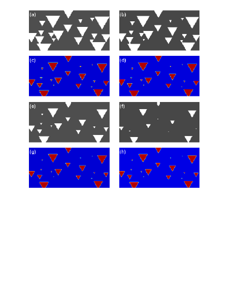
Figure 2: (color online). Simulated images of the $\phi$ and $\xi$ fields within the two-phase-field model. White triangles denote the $\phi$=1 islands and black background the $\phi$=-1 region in (a), (b), (e), and (f), and red (grey) triangles denote the $\xi$=1 islands and blue (black) background the $\xi$=-1 region in (c), (d), (g), and (h). The time interval is 200, 400, or 300 time steps between (a) and (b), (b) and (e), or (e) and (f), respectively, where 100 time steps are equal to 8 secondsl3 .

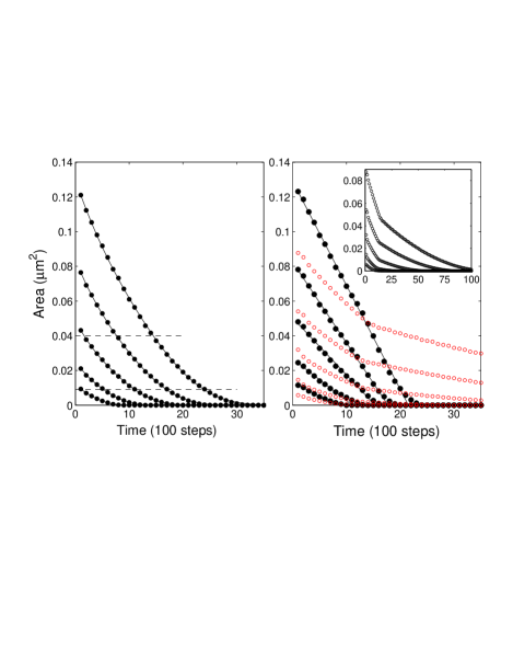
Figure 3: (color online). Simulated decay behaviors of five $\phi$=1 islands with initial areas $S_{0}$=0.1210, 0.0764, 0.0431, 0.0211, and 0.0093 $\mu m^{2}$ (from top to bottom) within the single phase-field model (left) and the two-phase-field model (right). In the left panel, the circle indicates the simulated island areas and the curve is fitted with the function $S_{0}\exp(-\alpha t-\beta t^{3.5})$. In the right panel, the filled (hollow) circles indicate the simulated areas of $\phi$=1 ($\xi$=1) islands and the lines are linearly fitted $\phi$=1 results. The inset shows the $\xi$=1 areas over the whole simulation time.

Main findings through simulation The simulated images are presented in Fig. 2. The whole time sequence of the 7$\times$7$\rightarrow$“1$\times$1” phase transition is shown in the eight panels (a-h), among which (a), (b), (e), and (f) for $\phi$ and (c), (d), (g), and (h) for $\xi$. At the beginning, the $\xi$=1 region is always enclosed in a larger $\phi$=1 region, as shown in the four panels (a)-(d). The $\xi$=1 region must be right in size with respect to the $\phi$=1 region in order to achieve the linear area decay behavior of the 7$\times$7 regions. Too small $\xi$=1 region is not enough to drive the decay from the exponential behavior, and on the other hand too large $\xi$=1 region overdrives the area decay from the linear behavior. The right area difference satisfies the condition that $S^{0}_{\phi}-S^{0}_{\xi}$ is a linear function of $S^{0}_{\phi}$. This can be understood by considering the fact that when the sample is quenched, the slow faulted stacking lags the formation of the dimers and corner holes.

The area decays for five islands are presented in the right panel of Fig. 3. The filled circles are the areas of $\phi$=1 islands and the hollow ones those of $\xi$=1 regions. The area decays are linear with time and the decay rates are 0.0060, 0.0046, 0.0031, 0.0021 and 0.0014 ($\mu$m² per 100 time steps) for the initial areas: 0.1210, 0.0764, 0.0431, 0.0211, and 0.0093 $\mu$m², respectively. It can be concluded that the area decay rate of a 7$\times$7 island increases with its initial area, being independent of its current area. An initially larger island always decays faster than an initially smaller one even when their sizes become equivalent to each other. The area decay rate of a 7$\times$7 island remains the same until the island disappears.

If using only one phase-field variable, we get area decay results shown in the left panel of Fig. 3. The filled circles show the areas of five islands with the same five initial areas as those of the two-phase-field model. They can be fitted with the function $S_{0}\exp(-\alpha t-\beta t^{3.5})$, with the parameters $\alpha$ and $\beta$ decreasing with $S_{0}$. Area decay rates of different 7$\times$7 islands increase with their current areas, not directly depending on their initial areas. The rate is 0.0047 $\mu$m² per 100 time steps at $S$=0.04$\mu$m² (upper dash line), and reduces to 0.0024 $\mu$m² per 100 time steps at $S$=0.01$\mu$m² (lower dash line). This behavior is not compatible with the experimental LEEM resultsl3 , and therefore the two phase-field variables are necessary to explaining the experiment.

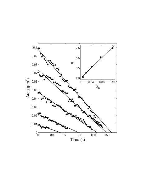
Figure 4: The two-phase-field simulated area decay (lines) of five 7$\times$7 islands compared with experimental LEEM data (dots)l3 . Inset: the simulated decay rate ($R$ in units of $10^{-4}\mu m^{2}/s$) vs the initial area $S_{0}$ ($\mu m^{2}$), where the squares, derived from Fig. 3, are fitted with a linear function.

Comparison with experiment In Fig. 4 we compare our simulated area decay results ($\phi$=1) in terms of the two-phase-field model with experimental data concerned. In the inset we present the relation of the area decay rate ($R$) with the initial area ($S_{0}$). We obtain a linear function, $R=0.00015+0.0051S_{0}$. With this function, the area decay rates are obtained by comparing the simulated island areas with experimental ones, or vice versa. The experimental island area $S$ can be described with a linear function of the time $t$, $S=S_{0}-Rt$. Because initial island area $S_{0}$ can be determined more accurately in LEEM experiment, we obtain $S_{0}$ by fitting experimental area data. The fitted $S_{0}$ are 0.0976, 0.0737, 0.0475, 0.0216, and 0.0090$\mu m^{2}$, and the corresponding area decay rates are 6.4, 5.2, 3.9, 2.6, and 2.0$\times 10^{-4}\mu m^{2}/s$. The theoretical linear behaviors are in good agreement with the experimental datal3 . Therefore, our theoretical model is very good for understanding the experimental results.

Conclusion We have proposed a natural two-speed model for the phase dynamics of the phase transition of Si(111) 7$\times$7 islands to unreconstructed high temperature “1$\times$1” phase. We formulate the phase dynamics by using phase-field method and adaptive mesh refinement technique. Our simulated results show that a 7$\times$7 island decays through step flow and the triangular shape is kept all the time. The decay rate of the island area is shown to be approximately a constant increasing with the initial area only. The LEEM experiments are explained quantitatively. This in return supports our conclusion: the corner holes and dimer chains are broken first and the remedying of the stacking-fault is slower and takes longer time. Therefore, the phase dynamics is elucidated. This phase-field theory is a reliable approach to studying the phase dynamics of general surface phase transitions.

- (1) W. Monch, Semiconductor Surfaces and Interfaces, Springer, Berlin 2001.
- (2) E. Kasper and D. J. Paul, Silicon quantum integrated circuits, Springer, Berlin 2005.
- (3) J. B. Hannon et al, Nature 440, 69 (2006).
- (4) Y. Sugimoto et al, Nature 446, 64 (2007).
- (5) I. Appelbaum et al, Nature 447, 295 (2007).
- (6) K. Takayanagi et al, Surf. Sci. 164, 367 (1985).
- (7) T. Hoshino et al, Phys. Rev. B 51, 14594 (1995).
- (8) T. Hoshino et al, Phys. Rev. Lett. 75, 2372 (1995).
- (9) W. Shimada and H. Tochihara, Surf. Sci. 526, 219 (2003).
- (10) F. J. Giessibl et al, Science 289, 422 (2000).
- (11) J. Kanamori and Y. Sakamoto, Surf. Sci. 242, 102 and 119 (1991).
- (12) S. Hasegawa et al, Phys. Rev. B 47, 9903 (1993).
- (13) T. Kato et al, Surf. Sci. 416, 112 (1998).
- (14) C.-W. Hu et al, Surf. Sci. 487, 191 (2001).
- (15) H. Hibino et al, Phys. Rev. B 72, 245424 (2005).
- (16) P. A. Bennett and M. W. Webb, Surf. Sci. 104, 74 (1981).
- (17) M. Itoh, Phys. Rev. B 54, 5873 (1996); 56, 3583 (1997).
- (18) W. Telieps and E. Bauer, Surf. Sci. 162, 163 (1985).
- (19) J. B. Hannon et al, Nature 405, 552 (2000).
- (20) J. B. Hannon et al, Phys. Rev. Lett. 86, 4871 (2001).
- (21) J. B. Hannon, J. Tersoff, and R. M. Tromp, Science 295, 299 (2002).
- (22) A. Karma and W. J. Rappel, Phys. Rev. E 53, R3017 (1996); Phys. Rev. Lett. 77, 4050 (1996); Phys. Rev. E 57, 4323 (1998).
- (23) A. Karma, Phys. Rev. Lett. 87, 115701 (2001).
- (24) F. Liu and H. Metiu, Phys. Rev. E. 49, 2601 (1994).
- (25) O. Pierre-Louis, Phys. Rev. E. 68, 021604 (2003).
- (26) Y.-M. Yu and B.-G. Liu, Phys. Rev. E 69, 021601 (2004); Phys. Rev. B 70, 205414 (2004); Phys. Rev. B 73, 035416 (2006).
- (27) D. D. Vvedensky, J. Phys. CM 16, R1537 (2004).
- (28) J. W. Evans, P. A. Thiel, and M. C. Bartelt, Surf. Sci. Rep. 61, 1 (2006).
- (29) N. Provatas, N. Goldenfeld, and J. Dantzig, Phys. Rev. Lett. 80, 3308 (1998); J. Comp. Phys. 148, 265 (1999).
- (30) Y.-N. Yang and E. D. Williams, Phys. Rev. Lett. 72, 1862 (1994).
- (31) Y. Fukaya and Y. Shigeta, Phys. Rev. Lett. 85, 5150 (2000).
- (32) W. Telieps and E. Bauer, Ultramicroscopy 17, 57 (1985).
- (33) S. Kohmoto and A. Ichimiya, Surf. Sci. 223, 400 (1989); T. Suzuki et al, Phys. Rev. B 59, 12305 (1999).
- (34) T. Hoshino et al, Surf. Sci. 394, 119 (1997).
- (35) E. Bauer, Rep. Prog. Phys. 57, 895 (1994).