Dots, clumps and filaments: the intermittent images of synchrotron emission in random magnetic fields of young supernova remnants

Abstract

Non-thermal X-ray emission in some supernova remnants originates from synchrotron radiation of ultra-relativistic particles in turbulent magnetic fields. We address the effect of a random magnetic field on synchrotron emission images and spectra. A random magnetic field is simulated to construct synchrotron emission maps of a source with a steady distribution of ultra-relativistic electrons. Non-steady localized structures (dots, clumps and filaments), in which the magnetic field reaches exceptionally high values, typically arise in the random field sample. These magnetic field concentrations dominate the synchrotron emission (integrated along the line of sight) from the highest energy electrons in the cut-off regime of the distribution, resulting in an evolving, intermittent, clumpy appearance. The simulated structures resemble those observed in X-ray images of some young supernova remnants. The lifetime of X-ray clumps can be short enough to be consistent with that observed even in the case of a steady particle distribution. The efficiency of synchrotron radiation from the cut-off regime in the electron spectrum is strongly enhanced in a turbulent field compared to emission from a uniform field of the same magnitude.

1. Introduction

The forward shocks of supernova remnants (SNRs) are the most probable accelerators of cosmic rays to high energies. Supporting this idea is the believe that the diffusive shock acceleration (DSA) mechanism is capable of accelerating particles to above 100 TeV in young and middle age SNRs. Electrons (and/or positrons) accelerated to $\sim\!10$ TeV will efficiently radiate in X-rays if magnetic fields exceed 100 $\mu$G. With Chandra’s imaging capability it is possible to distinguish the synchrotron structures in the X-ray images of Cas A, RCW 86, Kepler, Tycho and some other SNRs (e.g., Vink & Laming, 2003; Bamba et al., 2006; Patnaude & Fesen, 2008). The non-thermal emission seen by Chandra concentrates in very thin filaments in all SNRs. Bamba et al. (2006) also reported on the time evolution of the scale length of the filaments and roll-off frequency of the SNR spectra.

The synchrotron filamentary structures could be due to a narrow spatial extension of the highest energy electron population in the shock acceleration region limited by efficient synchrotron energy losses. In this case, strong magnetic field amplification in the shock vicinity is required to match the observed thickness of the non-thermal filaments (e.g., Vink & Laming, 2003; Bamba et al., 2005; Völk et al., 2005), thus supporting the case for highly efficient DSA. An alternative interpretation, that the observed narrow filaments are limited by magnetic field damping and not by the energy losses of the radiating electrons, was proposed by Pohl et al. (2005).

There is an emerging class of SNRs (SN1006, RXJ1713.72-3946, Vela Jr, etc) dominated by non-thermal X-ray emission. These SNRs are of particular interest since their X-ray emission most likely originates from synchrotron radiation of electrons accelerated to well above TeV energies. Many of the non-thermal X-ray SNRs are known to be radio-faint compared with most SNRs, and some of these remnants were first discovered in X-rays. The sources mentioned are now known to emit TeV photons as well and the origin of this emission is of fundamental importance for the origin of cosmic rays. Is it inverse-Compton emission from the X-ray emitting electrons, or pion-decay emission from proton-proton interactions, or both? One way to get the answer is to study the magnetic field structure in the SNRs.

Recently Uchiyama et al. (2007) reported variability of X-ray hot spots in the shell of SNR RXJ1713.72-3946 on $\sim$ one-year timescales. The authors suggested that this X-ray variability results from radiation losses and, therefore, reveals the ongoing shock-acceleration of electrons in real time. In order for radiation losses to be this rapid, the underlying magnetic field would need to be amplified by a factor of more than 100. From multi-wavelength data analysis Butt et al. (2008) concluded however, that the mG-scale magnetic fields estimated by Uchiyama et al. (2007) cannot span the whole non-thermal SNR shell, and if small regions of enhanced magnetic field do exist in RX J1713-3946, it is likely that they are embedded in a much weaker extended field. Therefore, it is essential to study the effects of magnetic field structure and particle distributions on the observed synchrotron emission maps.

Turbulent magnetic fields, with energy densities approaching a substantial fraction of the shock ram pressure, are a generic ingredient in the efficient DSA mechanism. However, the effect of turbulence on synchrotron emission images and spectra has not yet been addressed. In this paper, we model specific features in synchrotron images arising from the stochastic nature of magnetic fields. In §2 we describe our random magnetic field simulations, and these are used in §3 to construct synchrotron emission maps for different frequencies. Our results show that the rapid time variations seen in some SNRs may well be produced by steady electron distributions in turbulent fields.

2. Simulation of a random magnetic field

In order to simulate numerically an isotropic and spatially homogeneous turbulent field we sum over a large number ($N_{m}$) of plane waves with wave vector, polarization, and phase chosen randomly (see e.g. Giacalone & Jokipii, 1999; Casse et al., 2002; Candia & Roulet, 2004), i.e.,

$${\bf B}({\bf r},t)=\sum_{n=1}^{N_{m}}\sum_{\alpha=1}^{2}{\bf A}^{(\alpha)}(k_{n})\cos({\bf k}_{n}\cdot{\bf r}-\omega_{n}({\bf k}_{n})\cdot t+\phi_{n}^{(\alpha)})\ ,$$ (1)

where the two orthogonal polarizations ${\bf A}^{(\alpha)}(k_{n})$ ($\alpha=1,2$) are in the plane perpendicular to the wave vector direction (i.e., ${\bf A}^{(\alpha)}(k_{n})\perp{\bf k}_{n}$, so as to ensure that $\nabla\cdot{\bf B}=0$). We divided k-space between $k_{\mathrm{min}}=2\pi/L_{\mathrm{max}}$ and $k_{\mathrm{max}}=2\pi/L_{\mathrm{min}}$ into $N$ spherical shells distributed uniformly on a logarithmic scale (a number of points in the s-shell is $M_{s}$). Here $L_{\mathrm{min}}$ and $L_{\mathrm{max}}$ are the minimum and maximum scales of turbulence respectively. The spectral energy density of the magnetic field fluctuations is taken as $W(k)\propto k^{-\delta}$, where $\delta$ is the spectral index (c.f. Giacalone & Jokipii, 1999). The average square magnetic field $\langle B^{2}\rangle=\int dk\,W(k)$ is an input parameter for our model. In the particular simulation runs presented below we assume $\omega_{n}({\bf k}_{n})=v_{\rm ph}\cdot k_{n}$. The parameter $v_{\rm ph}$ would be a phase velocity in the case of a superposition of linear modes (e.g., magnetosonic waves). In this paper, however, we are modeling strong magnetic field fluctuations, so the random Fourier harmonics in Eq.(1) comprising the random field should not be exactly associated with any MHD eigen modes.

Following the prescription given above in Eq.(1), we simulated the temporal evolution of random magnetic fields filling a cube of scale size $D$, where $L_{\mathrm{min}}=2\times 10^{-4}\pi D$, $L_{\mathrm{max}}=0.2\,\pi D$, $N_{m}=4800$, and $N=6$, $M_{s}=800$. The choice of the mode number $N_{m}=4800$ provided the simulated fluctuation spectrum to be fitted with power law of index $\delta=1.0$ between $k_{\mathrm{min}}$ and $k_{\mathrm{max}}$ with accuracy better than 2$\%$. The spectral index $\delta=1$ corresponds to the so-called Bohm diffusion model in DSA. With the simulated random magnetic fields, we calculated the local spectral emissivity of polarized synchrotron emission at various times and for different distributions of electrons or positrons. The technique is described next along with the simulated emission maps.

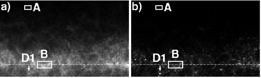
Figure 1.— Panels (a) and (b) are simulated maps of synchrotron emission in a random magnetic field. Intensities, $\nu^{2}\cdot I({\bf R_{\perp}},t,{\nu})$, are shown with a linear grayscale (white is maximum). The map (a) is made at 5 keV, while (b) is made at 50 keV. The shock position, where the electron distribution peaks, is indicated with a dashed line. The stochastic magnetic field sample has $\sqrt{\langle B^{2}\rangle}=10^{-4}$ G and $\delta=1.0$. A dim region “A” is marked to contrast a bright region ”B” and a dot marked as “D1”.

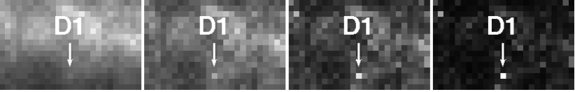
Figure 2.— Details of Fig.1 in the vicinity of the bright dot D1. The four panels show, from left to right, $\nu^{2}\cdot I({\bf R_{\perp}},t,{\nu})$ maps of synchrotron emission at 0.5, 5, 20 and 50 keV, respectively.

3. Synchrotron image simulations

The formation length $l_{f}$ of the synchrotron radiation pattern of an individual ultra-relativistic electron is energy independent, i.e., $l_{f}\approx R_{g}/\gamma=mc^{2}/eB\approx 1.8\times 10^{9}~{}B_{\mu G}^{-1}$ cm, where $R_{g}$ is the gyro-radius of a particle with Lorentz factor $\gamma$. The length $l_{f}$ is a small ($\gamma^{-1}$) fraction of the particle gyro-radius. In this study we only consider the effects of magnetic fluctuations having scales comparable to the gyro-radii of ultra-relativistic particles that are much larger than $l_{f}$. Therefore, the fluctuation wavenumbers $k$ satisfy $k\cdot l_{f}\ll$ 1. This restriction allows us to apply the standard formulae for the synchrotron power of a single particle of Lorentz factor $\gamma\gg 1$ in a homogeneous magnetic field, and then to integrate this power over the line of sight through the system filled with random field fluctuations.

We start with the spectral flux densities $p^{(1)}_{\nu}(\theta,E)$ and $p^{(2)}_{\nu}(\theta,E)$ with two principal directions of polarization radiated by a particle with energy $E$, given by Ginzburg & Syrovatskii (1965) [their Eqs.(2.20)]. Here $\theta$ is the angle between the local magnetic field ${\bf B}({\bf r},t)$ and the direction to the observer. In the case of a random magnetic field it is convenient to use the local spectral densities of the Stokes parameters (Ginzburg & Syrovatskii, 1965). A synchrotron map of a source can be constructed as a function of the position ${\bf R_{\perp}}$ in the plane perpendicular to the observer direction from the photons of a fixed frequency. Because of the additive property of the Stokes parameters for incoherent photons, we can integrate $p^{(1)}_{\nu}+p^{(2)}_{\nu}$ over the line of sight in the observer direction weighted with the distribution function of emitting particles $N({\bf r},E,t)$ to get intensity $I({\bf R_{\perp}},t,{\nu})$. To collect the photons reaching the source surface at the same moment, $t$, we performed the integration over the source depth using the retarded time $t^{\prime}=t-|{\bf r}-{\bf R_{\perp}}|/c$ as arguments in ${\bf B}({\bf r},t^{\prime})$ and $N({\bf r},E,t^{\prime})$. The integration grid had cell size smaller than $L_{\mathrm{min}}$. We produce the maps at different frequencies $\nu$ and for different times to study spectra and variability. Below we present synchrotron images simulated with a steady model distribution of electrons accelerated by a plane shock of velocity 2,000 $\rm~{}km~{}s^{-1}$ propagated in a fully ionized plasma of number density 0.1$\rm~{}cm^{-3}$. The kinetic model used to simulate the electron distribution was described in detail by bceu00. The magnetic field in the far-upstream region was fixed at 10 $\mu$G and it was assumed that magnetic field amplification produced a random field of $\sqrt{\langle B^{2}\rangle}=10^{-4}$ G in the shock vicinity. The effective shock compression ratio is about 4.7.

The spatial distribution of $\sim$ TeV electrons is highly non-uniform and concentrated near the shock due to synchrotron losses (see, also Zirakashvili & Aharonian, 2007). The simulated electron energy spectrum at the shock front position has asymptotic behavior $N\propto 7\times 10^{-12}[E/\mathrm{TeV}]^{-1.8}\exp[-(E/7\,\mathrm{TeV})^{2}]$ $\rm~{}cm^{-3}\,TeV^{-1}$ in the cut-off energy regime.

We note that, in reality, the distribution of the emitting electrons would be a random function of the position and particle energy because of the stochastic nature of both the electromagnetic fields and the particle dynamics. However, such a stochastic distribution can currently only be determined with particle-in-cell (PIC) simulations and then only for very limited energy ranges. The PIC simulation of TeV distributions in SNR shocks is beyond current computer capabilities (see, Vladimirov et al., 2008).

Our model highlights the effects of a stochastic magnetic field on the synchrotron mapping and demonstrates the importance of the high-energy cutoff region of the electron distribution where the synchrotron emissivity depends strongly on the local magnetic field.

4. Mapping of a synchrotron emission source

In this section we calculate maps of a synchrotron emission source with a random magnetic field. We use a set of parameters for a stochastic magnetic field sample with $\sqrt{\langle B^{2}\rangle}=10^{-4}$ G and $\delta=1.0$. Note that a 7 TeV electron has a characteristic synchrotron emission energy $h\nu_{\rm max}\approx$ 0.1 keV (calculated for a uniform magnetic field $B=10^{-4}$ G). However, this energy is not a good spectral characteristic in a random magnetic field because of the presence of the long tails in the probability distribution function (PDF) of the random field, as is clear in Figure 3. In Figure 1 we show $\nu^{2}\cdot I({\bf R_{\perp}},t,{\nu})$ maps at some particular time. Shock is propagating perpendicular to the line of sight direction. The 5 keV image (left panel a) clearly demonstrates the presence of structures: filaments, clumps and dots produced by the stochastic field topology. Filaments are less prominent at 50 keV (panel b), while dots and clumps are present. Polarization maps, where the degree of polarization is determined in a standard way also show clumpy structures. The degree of polarization reaches very high values in high energy clumps. We will discuss in detail the polarization properties of synchrotron structures and clump statistics elsewhere.

In Figure 2, the synchrotron emission of a small region around the dot D1 is shown for 0.5, 5, 20 and 50 keV. There are observable differences in the synchrotron maps indicating that some features are bright at high energies and much less prominent at lower energies and vice versa. The physical reason for this difference comes from the fact that in the high-energy cut-off region of the electron spectrum, the local synchrotron emissivity depends strongly on the local field value. High order statistical moments of the field dominate the synchrotron emissivity at high energies, and even a single strong local field maximum can produce a feature (dot or clump) that stands out on the map even after integrating the local emissivity over the line of sight. In lower energy maps, the contribution of a single maximum can be smoothed or washed out by contributions from a number of weaker field maxima integrated over the line of sight. The high energy map is highly intermittent because the synchrotron emissivity depends on high order moments of the random magnetic field at the cut-off frequency regime.

4.1. Spectra and temporal evolution of structures

In Figure 3 we show the simulated spectral density of the surface emissivity of a synchrotron source of size $D$ = 0.3 pc with the magnetic field model described above. The spectra for the regions of different surface emissivity apparent in Figure 1 are plotted separately in Figure 3. A dim rectangular region A and a bright dot D1 indicated in Figure 1 have drastically different spectra above 0.1 keV in the model. At the same time the spectrum of D1 is very similar to the total emissivity averaged over the whole map, indicating that the total emissivity is dominated by the bright dots and clumps.

The fact that bright dots and clumps contribute so strongly to the total emission means that there will be a clear spectral difference between the case where a source is filled with a uniform magnetic field (i.e., one equal to 0.1  mG in our simulation), and the case where the field is turbulent with $\sqrt{\langle B^{2}\rangle}=0.1$ mG, as we simulate in Fig.1. The presence of magnetic field fluctuations can substantially increase the synchrotron emissivity of electrons in the exponential tail of the distribution and if this effect is neglected, average magnetic fields may be inferred that are factors of several larger than is in fact the case.

An important aspect of synchrotron emission in turbulent fields is that the emission will vary in time even for a static electron distribution. In Figure 4 we show the relative intensity of the bright unresolved dot D1 [of size $\sim 10^{-2}D$] as a function of time measured in units of $D/v_{\mathrm{ph}}$, where $v_{\mathrm{ph}}$ is a characteristic speed of the magnetic turbulence, e.g., the Alfvèn speed. Figure 4 shows that a factor of two or more change in intensity will occur on times of a year if $D/v_{\rm ph}\sim 10^{10}$ s for X-rays with energies $\gtrsim 5$ keV. We simulate the image with minimal pixel size $10^{-2}D=10^{16}$ cm, while $L_{\mathrm{min}}$ was $6\times 10^{14}$ cm. For SNRs at kpc distances the simulated pixel size corresponds to the $\sim arcsecond$ range resolution of Chandra. The minimal variability time scale depends on the size of the structure $l$ if $l>L_{\mathrm{min}}$ and the dependence on $l$ is nonlinear since the photon emission is determined by high statistical moments of the random field in the cutoff regime. A one year variation-time of D1 at 5 keV requires $v_{\rm ph}\lesssim 10^{8}\rm~{}cm~{}s^{-1}$, which is a realistic value for the Alfvèn velocity for SNRs if the magnetic field is $\;\raise 1.29167pt\hbox{$>$\kern-7.5pt\raise-4.73611pt\hbox{$\sim$}}\;0.1$ mG. Figure 4 shows that higher energy X-rays in bright spots can vary on much shorter time scales, another consequence of emission from the exponential tail of the electron distribution. Some of the large scale filamentary structures seen in Fig.1 also show a complex time variability.

Figure 3.— Spectral densities of surface emissivity for regions in Fig. 1 as labeled. The solid curve is the average over the entire region shown in Fig. 1, while the dot-dashed curve is the spectrum produced if the region is filled with a uniform magnetic field of fixed magnitude $B$=10^-4 G, but of random direction.

Figure 4.— Temporal evolution of dot D1 shown in Fig.2 at 50 keV (dot-dashed curve), 20 keV (dashed curve), and 5 keV (solid line). The upper panel shows the evolution of D1 at 5 keV on a longer time scale.

5. Conclusions

We show that prominent, evolving, localized structures (e.g., dots, clumps and filaments) can appear in synchrotron maps of extended sources with random magnetic fields, even if the particle distribution is smooth and steady. The bright structures originate as high-energy electrons radiate efficiently in local enhancements of the magnetic field intensity. The peaks in synchrotron emission maps occur due to high-order moments of the magnetic field probability distribution function (PDF).

Even if the PDF of projections of the local magnetic field is nearly Gaussian, the corresponding PDF of synchrotron peaks, simulated for a spatially homogeneous relativistic particle distribution, has strong departures from the Gaussian at large intensity amplitudes. This is because of the non-linear dependence of the synchrotron emissivity on the local magnetic field in the high-energy cut-off regime of the electron spectrum.

Our model makes two basic predictions. One is that the overall efficiency of synchrotron radiation from the cut-off regime in the electron spectrum can be strongly enhanced in a turbulent field with some $\sqrt{\langle B^{2}\rangle}$, compared to emission from a uniform field, $B_{0}$, where $B_{0}=\sqrt{\langle B^{2}\rangle}$. The second is that strong variations in the brightness of small structures can occur on time scales much shorter than variations in the underlying particle distribution. The variability time scale is shorter for higher energy synchrotron images. Our estimate of the time scales of these intensity variations is consistent with the rapid time variability seen in some young SNRs by Chandra. The strong energy dependence we predict may be important for the future missions NuSTAR, Simbol-X and GRI that will image SNR shells up to 50 keV.

Non-thermal emission in many sources of interest such as gamma-ray bursts, AGNs and galaxy clusters originates from synchrotron radiation of ultra-relativistic particles in turbulent magnetic fields. The effect of random fields on synchrotron spectra and time evolution should be accounted for in their models. Relativistic flows in GRBs, PWNs and AGNs likely produce random magnetic fields with large amplitudes that should increase the efficiency of synchrotron radiation from electrons/positrons in the spectral cut-off regime.Synchrotron radiation in highly stochastic fields also results in energy band specific variability of the observed emission and its polarization. These specific characteristics of the synchrotron images and spectra in the cut-off regime can be used to study the turbulent magnetic fields in astrophysical sources.

References

- Bamba et al. (2005) Bamba, A., Yamazaki, R., Yoshida, T., Terasawa, T., & Koyama, K. 2005, ApJ, 621, 793
- Bamba et al. (2006) —. 2006, Advances in Space Research, 37, 1439
- Butt et al. (2008) Butt, Y. M., Porter, T. A., Katz, B., & Waxman, E. 2008, MNRAS, 386, L20
- Candia & Roulet (2004) Candia, J., & Roulet, E. 2004, Journal of Cosmology and Astro-Particle Physics, 10, 7
- Casse et al. (2002) Casse, F., Lemoine, M., & Pelletier, G. 2002, Phys. Rev. D, 65, 023002
- Giacalone & Jokipii (1999) Giacalone, J., & Jokipii, J. R. 1999, ApJ, 520, 204
- Ginzburg & Syrovatskii (1965) Ginzburg, V. L., & Syrovatskii, S. I. 1965, ARA&A, 3, 297
- Patnaude & Fesen (2008) Patnaude, D. J., & Fesen, R. A. 2008, ApJ (submitted) ArXiv 0808.0692
- Pohl et al. (2005) Pohl, M., Yan, H., & Lazarian, A. 2005, ApJ, 626, L101
- Uchiyama et al. (2007) Uchiyama, Y., Aharonian, F. A., Tanaka, T., Takahashi, T., & Maeda, Y. 2007, Nature, 449, 576
- Vink & Laming (2003) Vink, J., & Laming, J. M. 2003, ApJ, 584, 758
- Vladimirov et al. (2008) Vladimirov, A. E., Bykov, A. M., & Ellison, D. C. 2008, ApJ, 688, 1084
- Völk et al. (2005) Völk, H. J., Berezhko, E. G., & Ksenofontov, L. T. 2005, A&A, 433, 229
- Zirakashvili & Aharonian (2007) Zirakashvili, V. N., & Aharonian, F. 2007, A&A, 465, 695