Understanding the sub-critical transition to turbulence in wall flows

Abstract

Contrasting with free shear flows presenting velocity profiles with inflection points which cascade to turbulence in a relatively mild way, wall bounded flows are deprived of (inertial) instability modes at low Reynolds numbers and become turbulent in a much wilder way, most often marked by the coexistence of laminar and turbulent domains at intermediate Reynolds numbers, well below the range where (viscous) instabilities can show up [1, 2]. There can even be no unstable mode at all, as for plane Couette flow (pCf) or for Poiseuille pipe flow (Ppf) that currently are the subject of intense research. Though the mechanisms involved in the transition to turbulence in wall flows are now better understood [3], statistical properties of the transition itself are yet unsatisfactorily assessed. A widely accepted interpretation rests on nontrivial solutions of the Navier–Stokes equations in the form of unstable travelling waves [4, 5, 6, 7, 8] and on transient chaotic states associated to chaotic repellors [9]. Whether these concepts typical of the theory of temporal chaos are really appropriate is yet unclear owing to the fact that, strictly speaking, they apply when confinement in physical space is effective while the physical systems considered are rather extended in at least one space direction, so that spatiotemporal behaviour cannot be ruled out in the transitional regime. The case of pCf [10, 11, 12, 13] will be examined in this perspective through numerical simulations of a model with reduced cross-stream ($y$) dependence, focusing on the in-plane ($x,z$) space dependence of a few velocity amplitudes.[14] In the large aspect-ratio limit, the transition to turbulence takes place via spatiotemporal intermittency [15] and we shall attempt to make a connection with the theory of first order (thermodynamic) phase transitions, as suggested long ago by Y. Pomeau [16, 17].

Keywords. transition to turbulence, wall flows, sub-critical bifurcations
PACS Nos 47.27Cn, 47.27Lx, 47.20Ky

1 Introduction

The transition to turbulence is an important long standing problem owing to the marked difference between transport properties of laminar and turbulent flows but the process can follow different scenarios depending on the physical situation under consideration.

In closed flows, besides the instability mechanisms, e.g. Rayleigh–Bénard or Bénard–Marangoni for convection, Taylor–Couette for centrifugal flows [1], lateral effects play an important role. One can distinguish confined systems from extended ones. In confined systems, all the dimensions of the experimental cell are of the order of the length over which the mechanism operates, bifurcation theory applies to a limited set of central modes governed by normal forms obtained through adiabatic elimination of enslaved modes. The classical scenarios of transition to temporal chaos follow. In extended systems, at least one of the transverse dimensions is much larger than that in the direction selected by the instability mechanism and, while the latter still generates cells at a local scale, large scale modulations well described within the envelope formalism can degenerate into spatio-temporal chaos [18].

In open flows, the situation is more complex and less well understood. The natural control parameter is the Reynolds number $\mbox{Re}=\Delta U\Delta\ell/\nu$, where $\Delta\ell$ is the typical length scale, $\Delta U/\Delta\ell$ the typical shear in the system, and $\nu$ the kinematic viscosity measuring dissipation effects. At the linear stage [1, 2], standard stability analysis helps one classify base flow profiles into inflectional and non-inflectional (fig. 1). On general grounds, inflectional profiles become unstable and then turbulent through linear instability mechanisms of inertial origin (Kelvin–Helmholtz mechanism) at rather low Re and via cascading scenarios with mild super-critical flavour, i.e. with the bifurcated state staying in some sense close to the bifurcating one.

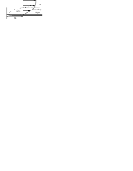
Figure 1: The wake of a blunt obstacle (left) and the boundary layer flow (right) are examples of inflectional and non-inflectional base flow profiles, respectively.

On the contrary non-inflectional flow profiles experience no instability at low Re but can possibly become unstable against subtle linear viscous mechanisms (Tollmien–Schlichting waves) at large $\mbox{Re}\geq\mbox{Re}_{\rm TS}$ only.

An essential assumption of linear stability analysis is the mathematically infinitesimal character of the perturbations. Relaxing this assumption one finds that, when $\mbox{Re}_{\rm TS}$ is large, the flow can depart from its laminar profile at values of $\mbox{Re}<\mbox{Re}_{\rm TS}$. Conditional stability is thus expected to be the rule for non-inflectional base flow profiles.

The physical role of advection in open flows is worth considering (fig. 2, left). Assuming a perturbation in the form of streamwise vortices (i.e. with axes aligned along the flow direction), it is immediately seen to induce flow corrections, called streaks, that are alternatively slowed down and accelerated with respect to the base flow. This mechanism, called lift-up, leads to transient perturbation energy growth even in linearly stable flows, thus plays a role in the direct transition to turbulence, and is an indisputable ingredient of the sustainment of turbulence in wall flows (fig. 2, right), see [3, 19].

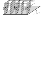
Figure 2: Left: Lift-up mechanism by which streamwise vortices induce alternatively slow and fast streaks. Right: Self-sustaining process in wall flows.

At the nonlinear stage, the by-pass scenario usually involves the nucleation and growth of turbulent spots embedded in linearly stable laminar flow. An example of turbulent domain (mature spot) immersed into laminar plane Couette flow (pCf) is given in figure 3 (left). Laminar-turbulent coexistence can be observed in other wall flows such as plane Poiseuille channel flow or the boundary layer flow. The shape and relative speed of spots depend on the case studied, see figure 1 of [10] for illustrations. Owing to the absence of overall advection and of TS instability mode ($\mbox{Re}_{\rm TS}=\infty$), plane Couette flow seems to be the simplest possible case to study. Poiseuille pipe flow (Ppf) is another classical example of flow that is always linearly stable [1] but becomes turbulent due to nonlinear perturbations. There, the coexistence of laminar and turbulent flows take the form of turbulent puffs becoming turbulent slugs at larger Re [20]. These systems have been the subject of intense study recently. Here we consider the case of pCf and keep in mind Ppf results [21, 22, 23] for comparison.

2 Phenomenology of plane Couette flow

Plane Couette flow is the flow ideally obtained by shearing a fluid between two infinite parallel plates at a distance $2h$ moving in opposite directions at speeds $\pm U$, which defines the streamwise direction $x$, $y$ and $z$ being the wall-normal and spanwise directions, respectively. The laminar profile is just $U_{\rm b}(y)=Uy/h$. It is known [1] to stay linearly stable for all values of the Reynolds number $\mbox{Re}=Uh/\nu$ ($\nu$ is the kinematic velocity) but, of course, to become turbulent for large enough Re. Here we summarise experimental results obtained by the Saclay group [24, 25, 11, 12, 13, 26, 10].

Basically, three kinds of experiments were performed: i₁) spot triggering, a tiny impulsive jet of controlled intensity is sent through the flow [24, 25, 13];

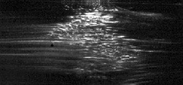
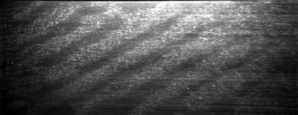
Figure 3: Left: spot in plane Couette flow at a late stage of its evolution; the streamwise direction is horizontal and the streaks are clearly visible; the hole through which the triggering jet is shot appears as a dark dot on the left of the picture’s centre (courtesy S. Bottin). Right: turbulent stripes at the upper end of the transitional regime (courtesy A. Prigent). In units of the half-gap $h$, the size of the set-up was $380h\times 2h\times 70h$ for the left snapshot and $770h\times 2h\times 340h$ for the right one.

i₂) quench experiments, turbulent flow is prepared at some initial high value of $\mbox{Re}_{\rm i}$ and Re is suddenly decreased to some final value $\mbox{Re}_{\rm f}$ [12, 13]; and ii) variable-strength permanent modifications to the base flow [11]. Experiments of kind (ii) which approach pure Couette flow by a continuation method confirm the results of experiments of kind (i) which are basically initial value problems. The bifurcation diagram given in figure 4 summarises the outcome of kind-(i) experiments:
– For $\mbox{Re}<\mbox{Re}_{\rm u}\simeq 280$, the laminar profile is rapidly recovered whatever the intensity of the perturbation brought to the flow.
– For $\mbox{Re}_{\rm u}<\mbox{Re}\lesssim\mbox{Re}_{\rm g}=325$, turbulence is only transient but as $\mbox{Re}_{\rm g}$ is approached from below, the lifetime of turbulence increases. For $\mbox{Re}_{\rm g}\lesssim\mbox{Re}\lesssim 360$ turbulence takes the form of irregular large spots (fig. 3, left). The actual status of $\mbox{Re}_{\rm g}$ is discussed in more detail below.
– For $360\lesssim\mbox{Re}\lesssim\mbox{Re}_{\rm t}=415$ the spots merge to form oblique stripes (fig. 3, right). These stripes are characterised by a regular modulation of the turbulence intensity which dies out when $\mbox{Re}_{\rm t}$ is approached from below, leaving one with a regime of featureless turbulence [26, 10].

Figure 4: Bifurcation of the plane Couette flow as obtained by the Saclay group.

Here we concentrate our attention on the lowest part of the transitional regime, i.e. $\mbox{Re}\lesssim 360$ where turbulent patches are not yet organised in oblique stripes. In the diagram, $\mbox{Re}_{\rm g}=325$ presents itself as the global stability threshold (‘g’ for ‘global’), i.e. the value of the control parameter below which the final state is always the laminar profile, whatever the amplitude of the initial triggering perturbation. Below $\mbox{Re}_{\rm g}$ turbulence is therefore not sustained. The lifetimes of transients were found to be distributed according to exponentially decreasing laws in the form $\mathcal{N}(\tau^{\prime}>\tau)\propto\exp(-\tau/\langle\tau\rangle)$, see figure 5 (left). The early proposal, made by Bottin and Chaté [13], that the characteristic times $\langle\tau\rangle$ of the distributions were diverging as $1/(\mbox{Re}_{\rm g}-\mbox{Re})$, was extracted from the results by simply taking the mean of the transients’ lifetimes at given Re (fig. 5, right). However, these results were somewhat noisy and $\mbox{Re}_{\rm g}$ was not approached sufficiently closely to make the conclusion decisive. The methodology giving $\langle\tau\rangle$ was further criticised by Hof et al. [21] who rather suggested the absence of a “critical” point and an exponential increase of the characteristic time with Re. This new proposal, made in close correspondence with their findings in the related problem of transitional Ppf, fully agrees with our reanalysis of the original data by fitting the terminal parts of the distributions in figure 5 (left) against straight lines. However the extrapolation of the exponential variation of the characteristic time with Re to much larger values may not be justified owing to the limited range of values studied.

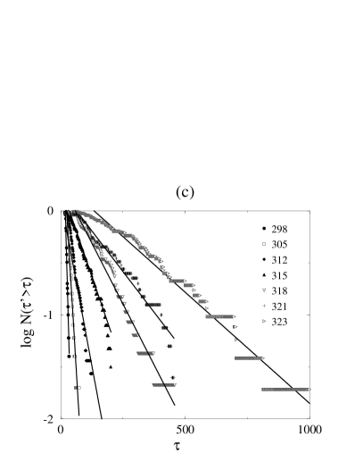
Figure 5: Left: distributions of transient lifetimes for a series of Reynolds numbers (quench experiments). Right: characteristic times extracted from these distributions as functions of Re. Courtesy S.Bottin.

According to Hof et al., transient behaviour with exponential distribution of lifetimes is associated to homoclinic tangles [9], themselves resulting from the presence of nontrivial unstable periodic orbits in a low dimensional dynamical systems perspective. Such solutions are known to exist both in Ppf [6, 7, 8] and in pCf [4, 5] and are furtively observed in experiments [7]. Since Poincaré’s work, the way a transverse intersection of stable and unstable manifolds of a limit cycle generates an uncountable infinity of intersections is well understood, as well as how complexity enters, through the symbolic dynamics attached to the modelling of that tangle in terms of Smale’s horseshoe. The exponential distribution of lifetimes of transient chaotic trajectories around the corresponding chaotic repellor then follows but, unfortunately, this nice application of the theory of low dimensional dynamical systems cannot predict how the slopes of the distributions vary with Re. In this respect, the case of pPf is not completely settled, some results displaying exponential behaviour [21], others a “critical” behaviour $\propto 1/(\mbox{Re}_{\rm g}-\mbox{Re})^{\alpha}$ for some global threshold $\mbox{Re}_{\rm g}$ with $\alpha\sim 1$ [22, 23]. A first reason explaining the observed discrepancies could be the experimental conditions since some experiments were performed at constant driving pressure gradient [21] and others at constant mass flux [22, 23]. As suggested by our results on plane Couette flow, another plausible possibility is linked to the fact that the physical system is not confined, but quasi-1D in physical space, i.e. confined in the radial direction, discretised in the azimuthal direction, but extended in the streamwise direction. Recent results from R.R. Kerswell and coll. (private communication) seem to point in that direction.

Taking for granted that the reduction of the dynamics to a 0D problem in physical space leaves aside interesting questions about the transitional regime in pCf, even more than in Ppf, we now study its dynamics in a quasi-2D spatiotemporal context, i.e. depending on space in the streamwise ($x$) and spanwise ($z$) directions, while keeping confinement conditions in the cross-flow direction ($y$).

3 Modelling transitional plane Couette flow

In contrast with most numerical studies restricting the system size by placing in-plane periodic boundary conditions at small distances (the size of the so-called minimal flow unit is typically $4\pi h\times 2h\times 2\pi h$ where $h$ is the half-gap [36]) and implicitly analysing the results in a finite-dimensional dynamical systems framework, experiments reported above were performed in domains at least as large as $380h\times 2h\times 70h$. Direct numerical simulations of the full Navier–Stokes equations in such domains are indeed not yet feasible with accuracy so that we have found it advisable to develop a spatiotemporal model. Instead of a set of differential equations governing scalar amplitudes (Lorenz-like model), the resulting model was a set of partial differential equations for a few fields (Swift–Hohenberg-like model). It was obtained from primitive equations (3D) through a systematic weighted residual approach, the Galerkin method, which uses a basis that fulfils the no-slip boundary conditions and projects the residuals on the same basis [31]. Here a simple polynomial basis was chosen and the expansion was truncated at lowest nontrivial order thus freezing most of the cross-flow space dependence, while leaving the in-plane dependence free. This was justified by the fact that, in the lowest part of the transitional regime, experimental and numerical evidence suggests the existence of coherent patterns occupying the full gap $2h$ with limited cross-stream structure [11, 30]. This restriction could of course be overcome but at a price of heavier analytical and numerical computations that we are not ready to pay for, since we mostly look for qualitative hints and not for quantitative agreement.

Due to the way it is obtained, the model a priori displays the problem’s most relevant general properties such as non-normal linear terms accounting for lift-up mechanism, linear viscous damping, nonlinear advection terms preserving perturbation kinetic energy, and linear stability of the base profile for all Re. Numerical simulations a posteriori show that it also shares many features of the complete physical system. In particular the statistics of homogeneous turbulent state no longer depends on the size of the simulation domain as soon as it is large enough (extensivity property) while the turbulent$\>\to\>$laminar transition is indeed discontinuous with exponentially distributed transient lifetimes [14].

Using this model, our main objective has been to contribute to “critical/exponential” controversy in the pCf case (with possible extrapolation to the Ppf case) and more particularly to point out the possible role of size effects.

3.1 Sub-criticality in the $32h\times 2h\times 32h$ system

In a first instance a $32h\times 2h\times 32h$ system has been considered, which is of moderate size when compared to the size of coherent structures $\sim 12h\times 2h\times 6h$ [19]. The state of the system was determined from its mean turbulent energy contents. The global stability threshold, with all the ambiguities the term covers, was determined by a combination of quench experiments, where Re is abruptly decreased from $\mbox{Re}_{\rm i}=200$ for which the flow is uniformly turbulent to variable $\mbox{Re}_{\rm f}\ll\mbox{Re}_{\rm i}$, and annealing experiments where Re was quasi-adiabatically decreased. As a result, turbulence seemed sustained for Re greater than $\approx 175$ but definitely transient for $\mbox{Re}<175$: the time series of the mean turbulent energy presented well distinct long plateaus before unpredictable sudden decay happened. Furthermore, the distributions of the transients’ lifetimes were clearly exponential and closely resembled the experimental ones depicted in figure 5 (left). The difference between the global threshold in the model $\mbox{Re}_{\rm g}\approx 175$ and in the laboratory $\mbox{Re}_{\rm g}\approx 325$ could be attributed to the under-estimation of viscous dissipation and energy transfer towards small cross-stream scales due to truncation. In spite of this lowering of the transitional regime by an empirical factor of about two, most qualitative aspects of nonlinear processes seemed preserved, e.g. those linked to the development of turbulent spots [32].

The variation with Re of the decay rate of the lifetime histograms is given in figure 6, which shows well aligned points in lin-log scale, hence exponential behaviour, except for $\mbox{Re}=174$ and $174.5$ which are mis-aligned. It turns out that this mis-alignment could not be explained by statistical errors, which suggests a crossover

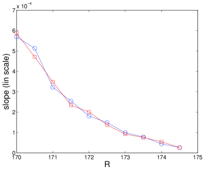
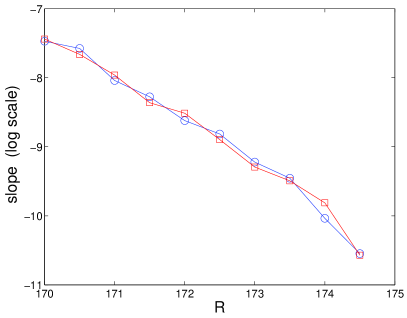
Figure 6: Decay rate of lifetime distributions as functions of Re in lin-lin scale (left) and in lin-log scale (right).

to critical behaviour very close to $\mbox{Re}=175$, possibly linked to size effects. Improving over this result was however beyond reach of numerical means and the visualisation of the velocity fields during decay did not help us discriminate between temporal and spatio-temporal behaviour.

In view of the typical size of streak segments mentioned earlier, temporal behaviour remained plausible in the $32h\times 2h\times 32h$ system. Expecting that this will no longer be the case when confinement effects are made weaker, we considered a much larger system of size $256h\times 2h\times 128h$.

3.2 Sub-criticality in the $256h\times 2h\times 128h$ system

Annealing experiments (Re decreasing quasi-adiabatically) first showed that turbulence could be maintained for very long times well below $\mbox{Re}_{\rm g}\simeq 175$ without any sign of decay. The time series of the mean turbulent energy shown in figure 7 (left) was

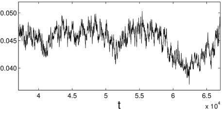
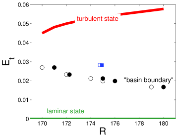
Figure 7: Left: Time series of the mean turbulent energy for the $256h\times 2h\times 128h$ system at $\mbox{Re}=170$. Right: Bifurcation diagram as obtained from the model in same system (full line: average mean turbulent energy during the adiabatic decrease of Re; open and filled dots: bracketing of the laminar/turbulent boundary for homogeneous low-level turbulent initial conditions; open and filled square: bracketing of the frontier at a single point for a strongly inhomogeneous initial state.

obtained in this way for $\mbox{Re}=170$. In contrast, relaxation at the end of a very long but regular and monotonic transient was observed for $\mbox{Re}=169$ without any trace of plateau indicating that turbulence could be metastable. So, at least down to $\mbox{Re}=170$ the turbulent state thus seems to be a local attractor and the continuous line in figure 7 (right) indicates the variation of the corresponding mean turbulent energy as a function of Re.

Visualisations of the turbulent pattern at $\mbox{Re}=170$ showed that, when the mean turbulent energy level was high, the system was in a state of fine-grained mixture of turbulent and laminar patches (spatiotemporal intermittency [15]), whereas during the excursions toward comparatively low values, large laminar domains were present for relatively long lapses of time. An explanation to the exponential behaviour of the lifetime distributions, alternative to the accepted one in terms of chaotic saddles, could then be obtained by considering the large $256h\times 2h\times 128h$ system as an assembly of 32 smaller $32h\times 2h\times 32h$ sub-systems and comparing the typical dynamics of the sub-systems to that of the $32h\times 2h\times 32h$ system [33]. Returning to the smaller system and comparing its time-series histograms at $\mbox{Re}=200$ to those at $\mbox{Re}=175$, it could be seen that an exponential tail appeared at low energy when Re was decreased, so that, when Re was further decreased, excursions toward smaller and smaller energies were more frequent, forcing the decay of a given transient when some limiting energy, $E_{\rm t}^{\rm lim}(32\times 32)\sim 0.025$, was reached. Setting this observation in the context of the sub-systems’ dynamics, one could then appeal to Pomeau’s analogy between sub-critical bifurcations in extended systems and first-order (thermodynamic) phase transitions [16] and the related theory of nucleation: The advent of a sizable laminar domain in the large system implies an excursion of the mean energy towards smaller values (e.g. $t~{}\sim 41000,\,51000,\,62500$ in fig. 7, left), though the system apparently remains in the sustained turbulent regime. Such excursions correspond to the breakdown of turbulence over regions already larger than the size of a sub-domain, which is also the size of the smaller system. Accordingly, while turbulence is relatively short-lived in the smaller system (since the occurrence of such a fluctuation would have led the turbulent regime to its end), it can be long-lived in the larger system because a wide region that fell laminar can become turbulent again by contamination from its surroundings. This observation opens the way to the understanding of the whole ‘turbulent $\to$ laminar’ transition in terms of directed percolation and statistical estimates that come with it [17].

The interpretation of the exponential decay of lifetime distributions in the smaller system thus rests on the idea that spatiotemporal fluctuations result in a random process exploring the low energy exponential tails of the mean turbulent energy histograms appearing when Re is small enough. While such a tail was indeed unobservable at $\mbox{Re}=200$, it was already sizable at $\mbox{Re}=175$, and quite substantial for $\mbox{Re}=170$ provided that the histogram was determined under the condition that the system is still in the chaotic transient state, i.e. as long as $E_{\rm t}>E_{\rm t}^{\rm lim}(32\times 32)$. The argument was closed by saying that the uniformly random exploration of the low-energy exponential histogram tails converted itself into exponentially decreasing lifetime histogram tails. Unfortunately, like the conventional view, this new interpretation does not predict how the lin-log slopes vary since it does not tell us how the tail’s importance changes with Re though the trend can be easily guessed. Invoking a spatiotemporal origin to the shape of the lifetime distribution could however help us understand the possible presence of a cross-over from exponential to critical variation.

Evidence that the turbulent state for $\mbox{Re}>170$ is a local attractor comes from the attempt to determine the frontier of its attraction basin as seen from the laminar $\to$ turbulent viewpoint. Open and filled dots in figure 7 (right) bracket the “line” separating random initial conditions with given initial mean turbulent energy obtained by attenuating the same homogeneous turbulent solution with variable factors. Above the line, the system evolves toward the turbulent state whereas it relaxes below. However the frontier appears to be strongly dependent on the shape of the initial condition and this dependence is better understood in physical space than in phase space. For example the open and filled squares in figure 7 (right) bracket the frontier corresponding to another kind of initial condition displaying wide laminar domains competing with the spatiotemporally intermittent state alluded to above. Still another frontier would be obtained for transverse turbulent stripes (parallel to the $z$ axis, not related to stripes in fig. 3) that are found to invade the system only when $\mbox{Re}>\mbox{Re}^{\perp}$, where $\mbox{Re}^{\perp}$ is the threshold value for spanwise turbulent stripes and happens to depend on the fraction $\alpha L_{x}$ of the system occupied by the stripe at the initial time (a single value $\alpha\approx 1/3$ has been studied, yielding $\mbox{Re}^{\perp}=195$). In the same way, strong localised perturbations form spots that make the whole system tumble into the turbulent state only for $\mbox{Re}>\mbox{Re}^{\rm spots}\sim 230$ but a precise determination of the corresponding threshold is barely feasible since it implies a three-parameter study by varying Re, the initial size and amplitude of the perturbation. Long range interactions associated to pressure effects, well accounted for in the model, also seem to play an important role.

To conclude, for decaying turbulence, the nucleation of sufficiently large laminar domains seems to provide a good understanding of the origin of the exponentially decreasing distribution of the transients’ lifetimes at given size, though a more complete study of the variation of the decay rates with Re combined with size effects is needed, which is currently underway. Though it has the same observable consequence as the saddle interpretation, this new approach clearly points to a spatiotemporal perspective that seems better suited than the strictly temporal one since spatial extension is a crucial feature of the problem. For onset, things are even much more complicated since the transition depends sensitively on the shape and amplitude of the initial condition and on the Reynolds number. Furthermore, it seems difficult to find a definite connection between our different results obtained in a spatiotemporal context and the search for edge states that have been much studied recently in a finite dimensional framework for both the pCf and the Ppf [34, 35, 36].

4 Conclusion

The transition to turbulence in wall flows leaves several problems open. Most difficulties stem from the nature of the non-trivial solution competing with the base state. Answers to this question have been looked for first within linear stability theory extended to take into account transient energy growth induced by non-normality, and next using the theory of nonlinear dynamical systems and temporal chaos. Accordingly, special periodic solutions (travelling waves) have been found, that serve as a skeleton for complex dynamics described in an abstract phase space in terms of homoclinic tangles and chaotic transients. This approach is however fully valid for confined systems and can only be applied to open systems at the price of putting artificial periodic boundary conditions at small distances in at least one (Ppf is quasi-1D), if not two (pCf is quasi-2D) directions of physical space. While the theory of chaotic transients well explains the exponential behaviour of the lifetime distributions, it does not account for the variation of their inverse decay rate with Re, which was found exponential in some cases and critical in others.

Taking another point of view, Pomeau long ago proposed an analogy of this kind of discontinuous bifurcation to a first-order (thermodynamic) phase transition [16] and put forward a related nucleation problem [17]. In the same time, he introduced the concept of transition to turbulence via spatiotemporal intermittency, a contamination process where above some threshold, activity invade the system whereas it dies below it [16]. The spatio-temporally intermittent state is a mixture of active and quiescent domains. Though at the time of the proposal, people focused mostly on the universality properties of the continuous transition [15], examples of discontinuous transitions were known. One of them was put in relation with the transition to turbulence in pCf [13] but the results were not reliable since the model was too far from concrete hydrodynamics. Keeping all this in mind, we developed a model which, instead of proceeding to full dimensional reduction in physical space, just froze part of the wall-normal dependence. In spite of an insufficient energy transfer through cross-stream (small) scales which led to a lowered transitional range, it correctly accounted for the interplay of streamwise vortices and streaks (large in-plane structures) and qualitatively reproduced hydrodynamical features, e.g. non-local pressure effects, and transitional properties. Even in the absence of firm conclusions (the work is still in progress), the most interesting results are a better appreciation of the drawbacks of the dynamical systems approach, and some support to the phase transition viewpoint. It indeed suggests a different interpretation of the transients’ lifetime distribution in systems of moderate size and offers a glimpse on the origin of complications arising from size effects and the role of topology of laminar/turbulent domains in pCf. The approach also suggests to look at Ppf along similar lines by considering it as a quasi-1D system and not as a 0D system in physical space.

Apart from perspectives open for other wall flows and flow control, the present approach and its spatiotemporal re-framing may help us better understand the nature of the turbulent attractor with respect to some “thermodynamic” approach to far-from-equilibrium systems to be defined in a firm statistical physics environment.

Acknowledgements:
It is my pleasure to thank people at LadHyX: M.Lagha (co-worker), C.Cossu, J.-M.Chomaz, P.Huerre, P.Schmid; at Saclay: S.Bottin, O.Dauchot, F.Daviaud, A.Prigent; at Marburg: B.Eckhardt, J.Schumacher; at ESPCI-Paris: L.Tuckerman, D.Barkley; at Bristol: R.R.Kerswell; at ENS-Paris: Y.Pomeau. All contributed at one level or another to my understanding of the problem but, of course, none should be taken responsible for the views expressed here. Large scale numerical simulations of the model were performed within the framework of projects #6/1462 and #6/2138 contracted with IDRIS-Orsay.

References

- [1] P.G.Drazin, W.H.Reid, Hydrodynamic Stability (Cambridge University Press, 1981).
- [2] P.Schmid, D.S.Henningson, Stability and Transition in Shear Flows (Springer, 2001).
- [3] T.Mullin, R.Kerswell, eds., IUTAM Symposium on Laminar-Turbulent Transition and Finite Amplitude Solutions (Springer, 2005).
- [4] G.Kawahara, S.Kida, J. Fluid Mech. 449, 291–300 (2001).
- [5] D.Viswanath, J. Fluid Mech. 580, 339–358 (2007).
- [6] H.Faisst, B.Eckhardt, Phys. Rev. Lett. 91, 224502 (2003).
- [7] B.Hof et al., Science 305, 1594–1598 (2004).
- [8] R.R.Kerswell, Nonlinearity 18, R17–R44 (2005).
- [9] B.Eckhardt, H.Faisst, “Dynamical systems and the transition to turbulence”, in [3], p.35–50.
- [10] A.Prigent and O.Dauchot, “Transition to versus from turbulence in subcritical Couette flows” in [3], p.195–219.
- [11] S.Bottin, O.Dauchot, F.Daviaud, P.Manneville, Phys. Fluids 10, 2597–2607 (1998).
- [12] S.Bottin, F.Daviaud, P.Manneville, O.Dauchot, Europhys.Lett. 43, 171–176 (1998).
- [13] S.Bottin, H.Chaté, Eur. Phys. J. B 6, 143–155 (1998).
- [14] M.Lagha, P.Manneville, Eur. Phys. J. B 58, 433–447 (2007).
- [15] H.Chaté, P.Manneville, “Spatiotemporal intermittency,” in Turbulence, a Tentative Sictionary, P.Tabeling, O.Cardoso, eds. (Plenum, 1995).
- [16] Y.Pomeau, Physica D 23, 3–11 (1986).
- [17] P.Bergé, Y.Pomeau, Ch.Vidal, L’Espace Chaotique (Hermann, 1998) Chapter IV [unfortunately available only in French].
- [18] P.Manneville, Dissipative Structures and Weak Turbulence (Academic Press, 1990).
- [19] F.Waleffe, J.Wang, “Transition threshold and the self-sustain ing process” in [3], p.85–106.
- [20] I.J.Wygnanski, F.H.Champagne, J. Fluid Mech. 59, 281–335 (1973).
- [21] B.Hof et al. Nature 443, 59–62 (2006).
- [22] J.Peixinho, T.Mullin, Phys. Rev. Lett. 96, 094501 (2006).
- [23] A.P.Willis, R.R.Kerswell, Phys. Rev. Lett. 98, 014501 (2007).
- [24] F.Daviaud, J.Hegseth, P.Bergé, Phys. Rev. Lett. 69, 2511–2514 (1992).
- [25] O.Dauchot, F.Daviaud, Europhys.Lett. 28, 225–230 (1994).
- [26] A.Prigent et al., Phys. Rev. Lett. 89, 014501 (2002).
- [27] N.Tillmark, P.H.Alfredsson, J. Fluid Mech. 235, 89–102 (1992).
- [28] A.Lundbladh, A.Johansson, J. Fluid Mech. 229, 499–516 (1991).
- [29] D.Barkley, L.Tuckerman, J. Fluid Mech. 576, 109–137 (2007).
- [30] O.Kitoh, K.Nakabyashi, F.Nishimura, J. Fluid Mech. 539, 199–227 (2005).
- [31] B.A.Finlayson, The Method of Weighted Residuals and Variational Principles, with Application in Fluid Mechanics, Heat and Mass Transfer (Academic Press, 1972).
- [32] M.Lagha, P.Manneville, Phys. Fluids 19, 094105 (2007).
- [33] P.Manneville, “Statistics of the laminar–turbulent transition in a model of plane Couette flow in extended geometry,” in preparation.
- [34] J.D.Skufca, J.A.Yorke, B.Eckhardt, Phys. Rev. Lett. 96, 174101 (2006).
- [35] T.M.Schneider, B.Eckhardt, J.A.Yorke, Phys. Rev. Lett. 99, 034502 (2007).
- [36] M.Lagha et al., “Laminar-turbulent boundary in plane Couette flow,” preprint.