Comments on “The long-period Galactic Cepheid RS Puppis. I. A geometric distance from its light echoes”

Abstract

Context. The luminous Galactic Cepheid RS Puppis is unique in being surrounded by a dust nebula illuminated by the variable light of the Cepheid. In a recent paper in this journal, Kervella et al. (2008) report a very precise geometric distance to RS Pup, based on measured phase lags of the light variations of individual knots in the reflection nebula.

Aims. In this commentary, we examine the validity of the distance measurement, as well as the reality of the spatial structure of the nebula determined by Feast (2008) based upon the phase lags of the knots.

Methods. Kervella et al. assumed that the illuminated dust knots lie, on average, in the plane of the sky (otherwise it is not possible to derive a geometric distance from direct imaging of light echoes). We consider the biasing introduced by the high efficiency of forward scattering.

Results. We conclude that most of the knots are in fact likely to lie in front of the plane of the sky, thus invalidating the Kervella et al. result. We also show that the flat equatorial disk structure determined by Feast is unlikely; instead, the morphology of the nebula is more probably bipolar, with a significant tilt of its axis with respect to the plane of the sky.

Conclusions. Although the Kervella et al. distance result is invalidated, we show that high-resolution polarimetric imaging has the potential to yield a valid geometric distance to this important Cepheid.

1 Introduction

RS Puppis (pulsation period 41.4 days) is one of the most luminous known Galactic Cepheids. It is thus a Milky Way analog of the bright Cepheids used to determine extragalactic distances, calibrate the brightnesses of Type Ia supernovae, and determine the Hubble constant. An accurate distance to RS Pup would provide a valuable anchor in setting the zero-point for the extragalactic distance scale and in determining whether there is a change in slope for the Cepheid period-luminosity relation (PLR) at long periods, as some authors have discussed (e.g., Ngeow et al. 2008 and references therein). Unfortunately, RS Pup is too far away for a trigonometric parallax measurement with existing instrumentation, even with the Fine Guidance Sensors onboard the Hubble Space Telescope (HST) (Benedict et al. 2007).

RS Pup is nearly unique among Galactic Cepheids in being embedded in a reflection nebula, as first pointed out by Westerlund (1961). Havlen (1972) demonstrated that features within the nebula show light variations at the Cepheid’s pulsation period and argued that these “echoes” could be used to derive a geometric distance. More recently, Kervella et al. (2008, hereafter K08) have used the 3.6-m ESO NTT telescope to monitor light variations within the nebula in excellent seeing. K08 were able to identify nearly three dozen nebular knots showing variations at the Cepheid period, of which the 10 best features were selected for analysis. By measuring the angular separations from the star, and determining the phase lags for each of these knots with respect to the stellar pulsation, they determined a geometric distance to RS Pup of $1992\pm 28$ pc. If valid, this would be by far the most precise distance measured for any Cepheid, Galactic or extragalactic (in terms of percent error), and it would provide a high-weight zero-point for the PLR, extragalactic distances, and $H_{0}$. It is important to examine the validity of this result, especially because it is about 15% higher than the 1728 pc found for RS Pup by Feast (2008) through application of the PLR of van Leeuwen et al. (2007); these latter authors have recently re-calibrated the zero-point on the basis of HST and revised Hipparcos trigonometric parallaxes of nearby Cepheids (none of which, however, have periods as long as that of RS Pup).

Unfortunately, in spite of the spectacular quality of their observations, we will demonstrate that K08’s analysis is based on an unjustified assumption that invalidates their result. We will argue that a geometric distance cannot be obtained from any direct imaging of the RS Pup nebula. However, we will also show that the addition of polarimetric imaging has the potential to enable a truly direct geometric distance determination for this important object.

2 Light-Echo Geometry

The geometry of a light echo is simple, in the case of a single flash from the illuminating star. At a time $t$ since outburst, the illuminated dust lies on the paraboloid given by $z=x^{2}/2ct-ct/2$, where $x$ is the projected separation from the star in the plane of the sky, and $z$ is the distance along the line of sight toward Earth. Thus the outer parts of the echo usually correspond to dust in front of the star, and the inner parts to dust behind the star. Because of the geometry, the outer parts of a light echo generally appear to expand at a speed much greater than the speed of light.

The most spectacular light echo in astronomical history is on display around the exotic variable star V838 Monocerotis (Bond et al. 2003; Corradi & Munari 2007), imaged extensively by HST (Bond 2007). Direct imaging of the echo cannot yield a geometric distance. However, polarimetric imaging can identify the region within the echo where the linear polarization is maximum, marking the location where the scattering angle toward the Earth is $90^{\circ}$. This highly polarized light corresponds to dust lying in the plane of the sky, where the light-echo equation shows that the linear distance from the star is $x=ct$. The angular separation of this location from the star then yields the geometric distance. This novel method for astronomical distance determination was first spelled out by Sparks (1994). Sparks et al. (2008, hereafter S08) have now applied the method to HST polarimetric images of V838 Mon obtained in 2002–5. They indeed detected a ring of highly polarized light expanding at the speed of light, and found a distance of $6.1\pm 0.6$ kpc. This determination has been verified independently through classical main-sequence fitting for a sparse stellar cluster associated with V838 Mon by Afşar & Bond (2007), yielding a distance of $6.2\pm 1.2$ kpc.

3 The Nested Light Echoes of RS Puppis

The light-echo situation is far more complicated when the illuminating source is a periodic variable star. In this case, as seen from Earth, a train of nested paraboloids propagates outward into the surrounding dust. This geometry is illustrated in Fig. 1. The illumination seen at a given projected separation, $x$, from the star will be the integral along the line of sight of the incident intensity at each $z$ location (a function of the corresponding phase of the Cepheid variation), modified by the dust density at each volume element, by $r^{-2}$, where $r$ is the distance of that volume element from the star, and by the dust scattering phase function $\Phi(\xi)$, where $\xi$ is the scattering angle (taken to be $0^{\circ}$ for forward scattering). See S08 for a detailed discussion of such calculations and references to earlier literature.

Fig. 1 thus demonstrates that, for a uniformly filled nebula, the light variations will largely average out over the line of sight, since all phases of the light variation are covered multiple times. Only if there is a non-uniform distribution of dust along the line of sight (for example, isolated nebular knots, or a very non-spherical nebular morphology) will we see high-amplitude periodic light variations at those locations. K08 in fact did confirm the work of Havlen by demonstrating the existence of locations in the nebula where there are such variations.

However, even for such isolated knots, there is an unavoidable ambiguity in their $z$ locations. Referring again to Fig. 1, let us consider the brightest variable knot found by K08, which is “Knot 5” in their Table 3. It lies at a separation of $x=16\aas@@fstack{\prime\prime}03$ from the star, marked as a vertical dashed straight line in Fig. 1. The fractional phase lag of Knot 5 is observed to be 0.504, i.e., its light maxima lag about 20.9 days behind those of RS Pup itself. Thus its $z$ location must lie halfway between a pair of parabolas along the straight line in Fig. 1, but we do not know which pair! The knot could lie $\sim$0.23 pc in front of the plane of the sky (phase lag 1.504 cycles), or 0.10 pc (2.504 cycles), or 0.02 pc (3.504 cycles), or in the plane of the sky (4.504 cycles), or 0.02 pc behind (5.504 cycles), etc. (The $z$ distances given here depend, of course, on the assumed stellar distance, in this case 2 kpc.) When the only observations available are direct images, there is no way to resolve this uncertainty without making arbitrary assumptions.

K08 resolved the ambiguity by assuming the knots to lie in the plane of the sky. Under this assumption, and making an initial guess at the distance to the star, the integer numbers of cycles in the phase lags become known (in the case of Knot 5, it is 4). Then the fractional phase lag for each knot yields a stellar distance, and the final result was taken as the mean of the distances determined from 10 individual features, i.e., $1992\pm 28$ pc.

K08 recognized that the assumption that the knots lie in the plane of the sky would generally not be true for any particular individual knot, but argued that the assumption would be true in the mean, as long as the spatial distribution of the knots is close to isotropic.

4 Critiques of the K08 Analysis

4.1 Summary of K08 Analysis Procedure

The RS Pup nebula was imaged by K08 using the 3.6-m European Southern Observatory New Technology Telescope (NTT) and the ESO Multi-Mode Instrument (EMMI). CCD images were obtained on 7 nights between 2006 October and 2007 March, in seeing generally ranging from $0\aas@@fstack{\prime\prime}8$ to $1\aas@@fstack{\prime\prime}1$.

The analysis procedure employed by K08, based on their superb time series of high-resolution images of the nebula, is first to isolate a set of locations within the nebula where there are light variations at the Cepheid’s pulsation period, and where the amplitudes of the variations are large and comparable to that of the Cepheid itself. The large amplitude ensures that the knot is isolated and that additional material elsewhere along the line of sight, and thus out of phase, is not significantly diluting the variations. K08 identified 10 prominent features that satisfied these criteria, as well as a larger number of lower-weight knots.

At each such location in the nebula, there are two observables: the angular separation of the knot from the star, and the phase lag of its light curve relative to RS Pup. In the notation of K08, the angular separation of knot $i$ is $\theta_{i}$, and its phase lag consists of an integer number of periods, $N_{i}$ (which is unknown), plus a fractional lag, $\Delta\phi_{i}$, determined from the amount of time by which the echo light curve is out of phase with the Cepheid.

With these two observables, the K08 procedure is to assume that the knot lies in the plane of the sky, adopt an initial estimate of the distance $d$, and then derive the integer number of periods in the time delay, according to $N_{i}={\rm int}(\theta_{i}\,d/cP)$, where $c$ is the speed of light and $P$ is the pulsation period of the Cepheid. Once $N_{i}$ is known for each knot, a distance, $d_{i}$, is obtained based on each one, using $d_{i}=(N_{i}+\Delta\phi_{i})P/c\theta_{i}$. If $\theta_{i}$ is in arcseconds, and $P$ in days, this equation becomes $d_{i}=(N_{i}+\Delta\phi_{i})P/(5.7755\times 10^{-3}\,\theta_{i})\,\rm pc$. K08 adopt a period of $P=41.4389$ days.

Using these equations, K08 stepped through a range of initial estimates of $d$, calculated $N_{i}$ and the corresponding $d_{i}$ for each knot, and then derived the standard deviation of the $d_{i}$ values. They found a deep minimum of the dispersion of the distance estimates at a weighted value of $1992\pm 28$ pc, as discussed in detail in their paper.

4.2 Statistical Significance

We first present a simple test of the statistical significance of the above result, which was based on searching for the minimum standard deviation of the distance estimates. We follow the procedure of K08, namely stepping through a range of starting values of the distance, and calculating the relative standard deviation (the standard deviation divided by the mean distance) at each assumed distance. We use the set of 10 high-weight pairs of $\theta_{i},\Delta\phi_{i}$ values given by K08 (their Table 3), and follow their procedure of deleting the two lowest and two highest values of $d_{i}$ before calculating the mean and standard deviation. The top left panel in Fig. 2 plots the relative standard deviation vs. assumed distance for the K08 data. This plot shows a minimum relative standard deviation of 1.6% at a distance of 1975 pc (K08 give 1.1% at 1992 pc, due presumably to a slightly different weighting and/or deletion scheme).

To test the significance of this result, we tried the experiment of adopting the same set of 10 values of $\theta_{i}$, but assigned phase lags, $\Delta\phi_{i}$, generated by a random-number routine that outputs values in the 0.00–1.00 range. We ran this experiment 9 times, and plot the results in the remaining 9 panels in Fig. 2. As the panels show, two-thirds of these randomizations (6 out of 9) show lower minima than the 1.6% obtained for the actual data. (The lowest minimum found in the range 0 to 3000 pc was a relative standard deviation of only 0.6% in the 8th randomization, at a distance of 2380 pc.)

We believe that this simple experiment demonstrates very low statistical significance for the distance of 1992 pc found by K08 through minimizing the relative standard deviation of the distance estimates. Note that the relative standard deviation systematically trends downward with increasing assumed distance. This arises naturally because the cycle count, $N_{i}$, increases with assumed distance, but the phase lags can never vary by more than $\pm$0.5; thus the percentage scatter in the derived distances decreases systematically with distance.

4.3 Biasing Away from the Plane of the Sky

However, there is a more fundamental objection to the K08 analysis. Unfortunately, the assumption that the light-variable knots are in the plane of the sky is quite unlikely to be true, not even in the mean, and not even if the knots are distributed isotropically around the star. In fact, we expect a strong biasing such that the brighter knots are likely to lie in front of the plane of the sky, because of the behavior of the scattering phase function $\Phi(\xi)$.

This phase function is usually taken to be that of Henyey & Greenstein (1941): $\Phi(\xi)=(1-g^{2})/[4\pi(1+g^{2}-2g\cos\xi)^{3/2}]$, in which the parameter $g$ for interstellar dust is empirically found to be near $g=0.6$ (see references in S08). In this case, for example, the relative scattering efficiencies for angles of $0^{\circ}$, $15^{\circ}$, $30^{\circ}$, $45^{\circ}$, $90^{\circ}$, and $180^{\circ}$ are 1, 0.71, 0.35, 0.17, 0.04, and 0.016. Thus knots with smaller scattering angles will be systematically brighter, and as Fig. 1 shows these knots are preferentially in the foreground. Hence the high efficiency of forward scattering imposes an unavoidable biasing away from knots lying in the plane of the sky.

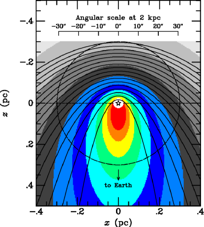
Figure 3: This figure repeats Fig. 1, with overplotted contours indicating the value at each $(x,z)$ point of the scattering function, $\Phi(\xi)$, divided by $r^{2}$, the square of the distance from the star. This ratio, multiplied by the local dust density, is proportional to the contribution to the surface brightness at a given line of sight along the $z$-direction as seen from Earth. Each contour represents a step of a factor of 2 in $\Phi(\xi)/r^{2}$. The strong biasing toward the brightest nebular knots lying in the foreground is illustrated. The horizontal line at $z=0$ marks the plane of the sky.

A quantitative illustration of this biasing is shown in Fig. 3. Here we have taken Fig. 1 and superposed regions that are color-coded according to the local values of $\Phi(\xi)/r^{2}$, where $\Phi(\xi)$ is the dust scattering efficiency described above, with $g=0.6$, and $r$ is the distance of the volume element from the star. Thus this function, multiplied by the local volume density of dust, is proportional to the observed surface brightness at that location in the nebula as seen from Earth. The contours between the colored regions correspond to steps of factors of 2 in $\Phi(\xi)/r^{2}$. To interpret the figure, consider for example a dust knot located at a projected separation of $x\simeq 0.15$ pc from the star, typical of the variable features found by K08. The same knot, if located $\sim$0.15 pc in front of the plane of the sky would be about 2 times brighter than if it were located in the plane, and about 9 times brighter than if it were located $\sim$0.15 pc behind the plane. At $x\simeq 0.1$ pc, a knot located $\sim$0.25 pc in front of the plane of the sky would be 1.8 times brighter than if in the plane of the sky, and 32 times brighter than the same knot located 0.25 pc behind the plane. More generally, there are large extents along the positive $z$ direction of nearly constant brightness, but once the plane of the sky is crossed the brightness drops very rapidly.

There is also a second and more subtle effect that likewise biases the variable knots toward lying in front of the plane of the sky. For a knot to show a large-amplitude light variation, it must be spatially isolated so as not to have its variation diluted by scattering from other material in the same line of sight, illuminated by light with a range of different phase lags. As Figs. 1 and 3 illustrate, the echo paraboloids become more closely spaced in the $z$-direction as we move down the line of sight. This means that a knot with the same linear extent along the line of sight will suffer increasingly more phase dilution as it is placed at successively greater distances from the observer along the $z$-axis.

Because of this strong biasing of the illuminated and high-amplitude knots to lie in the foreground, the assumption of K08 that they lie in the plane of the sky appears unjustified. When this assumption has to be abandoned, it is no longer possible to derive a geometric distance from the phase lags.

The assumption that a knot lies in the plane of the sky when it in fact does not will lead to very large errors in the derived distances. For a concrete example, we consider again Knot 5, lying at $\theta_{5}=16\aas@@fstack{\prime\prime}03$, which was discussed in §3. If this knot is assumed to lie in the plane of the sky, the distance will be calculated to be 673, 1120, 1568, and 2015 pc, for adopted values of $N_{5}$ of 1, 2, 3, and 4, respectively. K08 had assumed $N_{5}=4$. Actually, as shown in Fig. 3, Knot 5 is statistically likely to lie $\sim$0.2 pc in front of the plane of the sky and to have $N_{5}\simeq 1$ (if the distance to the star is of order 2 kpc).

5 Three-Dimensional Structure of the RS Puppis Nebula

5.1 Equatorial Disk?

In a paper that came to our attention as we were completing this critique, Feast (2008) discusses the results of K08 and reaches the same conclusion that we do, namely that the assumption that the echo knots lie in the plane of the sky is unjustified.

Feast then essentially reverses the analysis of K08, using the measured phase lags in order to study the three-dimensional distribution of the light-variable nebular knots. He assumes a distance to RS Pup of 1728 pc based on the PLR, and then uses the $\Delta\phi_{i}$ values to solve for the $z$ locations of each of the knots. If the knots are not in the plane of the sky, the equation in §4.1 becomes $(N_{i}+\Delta\phi_{i})=5.7755\times 10^{-3}D\,\theta_{i}(1+\sin\alpha_{i})/P\cos\alpha_{i}$, where $D$ is the distance to the star in pc, and the angle $\alpha_{i}$ is, in our notation, given by $\alpha_{i}=-\tan^{-1}z_{i}/x_{i}$. This equation can be solved to obtain a $z$ depth for each illuminated knot. Of course, a unique solution is not possible, as the $z$ location depends on the arbitrarily chosen integer number of cycles in the phase lag, $N_{i}$. Feast was, however, able to find a particular set of values of $N_{i}$, slightly modified from those obtained by K08 who assumed the knots to lie in the plane of the sky, which places the knots on the north side of the star in front of, and those on the south side behind, the plane of the sky. In his solution, the knots lie close to an inclined plane, which he interprets as indicating that the nebula is a highly flattened disk, tilted by only $8\aas@@fstack{\circ}1$ to the plane of the sky. In the top panel of Fig. 4 we have reproduced Feast’s Fig. 1, except that we use the same scale for both coordinates so as to show the correct proportions. Feast’s calculations were made for an expanded set of data for 31 knots, provided by Kervella to Feast and reproduced in the latter’s Table 1. In Feast’s notation, $d_{y}$ is our $-z$, and $d_{x}$ is the projected separation of the knot from the line where the plane of the disk intersects the plane of the sky, given by $d_{x}=0.008377\,\theta_{i}\sin(\beta_{i}-\gamma)$ pc, where $\beta_{i}$ is the position angle (PA) of the knot, and $\gamma$ is the azimuth at which the plane of the disk cuts the plane of the sky, taken by Feast to be $80^{\circ}$.

Feast’s result is surprising because most of the knots are found to be behind the plane of the sky, contrary to the expectation established here that they should preferentially lie in the foreground. However, Feast’s conclusions are entirely dependent upon an arbitrary assumption of values of $N_{i}$ that are large on the north side, and smaller on the south side, in order to yield this tilted geometry. To illustrate the arbitrary nature of this analysis, we repeated his calculations with our own set of $N_{i}$ values. By visual inspection of the K08 image of the nebula, it appears to us that there is a long axis oriented at a PA of about $35^{\circ}$, which would imply $\gamma=125^{\circ}$. With this new value, and by a process of trial and error, we were easily able to obtain a new set of $N_{i}$ values that gives the plane containing the knots the opposite tilt and nearly the same level of scatter, as Feast’s fit. Our plot is shown in the middle panel of Fig. 4.

This exercise primarily serves to demonstrate that there is no unique three-dimensional structure that can be inferred from the set of $\theta,\Delta\phi$ pairs. Our result does have the advantage that the knots on the south side of the nebula, where they are brightest (see below), are well in front of the plane of the sky. However, as we argue in the next subsection, it is more likely that the nebula actually has a pronounced bipolar morphology.

5.2 Bipolar Nebula?

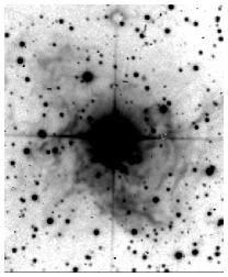
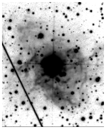
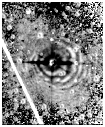
Figure 5: The first two panels are ESO 3.6-m CCD images of RS Pup obtained on 1995 March 5 and May 4, a time separation of 1.44 Cepheid cycles. The third panel shows the ratio of the two images. Stretches for the two direct images are logarithmic, and linear for the ratio image. In the ratio image, white marks regions brighter in May than March. North is at the top, east is on the left, and the frames are $160^{\prime\prime}$ wide. There is a bright satellite streak in the May image.

We can gain a general idea of the overall morphology and orientation with respect to the plane of the sky of the RS Pup nebula through ratio imaging. As a preliminary example of how such a study might proceed, we present in Fig. 5 two images of the nebula, obtained by W.B.S. with the 3.6-m ESO NTT and EFOSC CCD coronagraphic imager on 1995 March 5 and May 4. The time interval between the images was 59.86 days, or 1.44 cycles of the Cepheid.

The first two frames in Fig. 5 show the two direct images. They were obtained with an $R$ filter combined with polarizers at four different electric-vector angles, and these images are the sums of the four. The third frame in Fig. 5 shows the ratio of the May and March images, with an image stretch in the sense that white represents areas that were brighter in May and black represents areas that were fainter. The reflected light variations due to the Cepheid are clearly visible, as a series of bright and dark elliptical rings, most prominently on the SW side.

Although these images ($\rm FWHM\simeq 1\aas@@fstack{\prime\prime}5$) do not have seeing as excellent as the K08 frames, they reveal some important large-scale morphological properties. First, the direct images show that the nebula is elongated in the NE-SW direction, along a PA of about $35^{\circ}$. Second, the surface brightness is generally higher on the SW side of the star than it is on the NE. This is the appearance we would expect if the nebula has an overall cylindrical (or bipolar) structure, tilted such that the SW lobe is in front of the plane of the sky (giving it a relatively high surface brightness because of the smaller scattering angle), and the NE lobe is behind the plane of the sky (large scattering angle and lower surface brightness).

The elliptical rings seen in the ratio image in Fig. 5 strongly support this interpretation. First, as noted in §3, light variations will be averaged out if there is an appreciable depth along the line of sight. Thus, the prominent variations on the SW side indicate that there is a limited $z$-direction extent of the nebula, i.e., it is not spherical. Moreover, on the SW side, the arcs have the widest spacing, indicating a relatively wide spacing between the paraboloids in the $x$ direction. As Fig. 1 shows, this wide spacing occurs in the foreground. At least five separate rings can be seen on this side of the star, again showing that this material must lie well in front of the plane of the sky. By contrast, the rings are more closely spaced, and fade away rapidly, on the NE side. This strongly suggests that the material here is in the background, where the paraboloids are much more closely spaced in the $z$ direction, causing the light variations to average out.

The first, second, and third bright rings in the ratio image, where their spacing is largest on the SW side, lie at radii of $\sim$$18^{\prime\prime}$, $34^{\prime\prime}$, and $46^{\prime\prime}$. This suggests that the number of cycles in the lags is increasing in steps of 1 at each of those radii [e.g., if the first frame had been taken at a time of maximum of the Cepheid, the values of $(N_{i}+\Delta\phi_{i})$ could be 0.44, 1.44, and 2.44 at these rings; or, if the first ring is too close to the star to be resolved, the values could be 1.44, 2.44, and 3.44].

To give an indication of the orientation of the nebula suggested by these features, we repeated the analysis of the previous subsection, again adopting $\gamma=125^{\circ}$. For the 11 knots lying in the third quadrant ($180^{\circ}<\beta<270^{\circ}$), guided by the ring radii given above but with some degree of arbitrariness, we set $N_{i}=1$ if $10\aas@@fstack{\prime\prime}96<\theta_{i}<17^{\prime\prime}$, $N_{i}=2$ if $17^{\prime\prime}<\theta_{i}<30^{\prime\prime}$, and $N_{i}=3$ if $\theta_{i}>30^{\prime\prime}$. These choices place those knots well in front of the plane of the sky, as expected. We then artibrarily adjusted the $N_{i}$ values for the remainder of the 31 features so that they generally fall along the plane established by the third-quadrant knots. The resulting spatial distribution is plotted in the bottom panel of Fig. 4. This rendition is consistent with all of the expectations, i.e., most of the variable knots found by K08 lie in the foreground, most of them lie on the SW side of the star (positive values of $d_{x}$) where the nebula is brightest, and the knots in the SW quadrant have low values of $N_{i}$ ranging from 1 to 3. For this set of $N_{i}$ values, the axis of the bipolar structure is tilted by about $40^{\circ}$ with respect to the plane of the sky; but we emphasize that the $N_{i}$ values for most of the knots were chosen arbitrarily to yield a flattened distribution. The variable knots in the background are, actually, more probably those on the front surface of the bipolar structure rather than along its axis as shown.

6 Polarimetry to the Rescue

We have shown that the precise distance determination of K08 is invalidated by the unjustified assumption that the variable dust knots in the RS Pup nebula lie in the plane of the sky. In fact, we demonstrated that the nebula is plausibly an elongated struture, highly tilted with respect to the plane of the sky.

Fortunately, the use of polarimetric imaging, at HST resolution, has the potential to yield a geometric distance, much as it did for V838 Mon (see S08). The degree of polarization of scattered light, $p$, depends strongly on the scattering angle $\xi$, according to the classical Rayleigh function, $p=p_{\rm max}\,(1-\cos^{2}\xi)/(1+\cos^{2}\xi)$, which has its maximum value at $\xi=90^{\circ}$. In the case of the V838 Mon echo, S08 indeed found a high degree of linear polarization, $p_{\rm max}\simeq 50\%$, at the $90^{\circ}$ scattering angle, from which they obtained a geometric distance to V838 Mon. As described above (§2), this distance has been verified independently through a distance determination based on main-sequence fitting.

We thus have a simple recipe for determining a true geometric distance to RS Pup:

1. Obtain imaging polarimetry of the nebula over a 41.4-day pulsation cycle, using the polarimetric mode of HST’s Advanced Camera for Surveys (ACS; scheduled to be restored to service during the upcoming Servicing Mission 4). Search the images for small knots that (a) vary with the full light amplitude of the Cepheid variation (showing that they are indeed isolated along the line of sight), (b) have the highest degree of linear polarization (demonstrating that they lie near the plane of the sky), and (c) have a constant degree of polarization over the pulsation cycle (showing again that the line of sight is undiluted by contributions from out of the plane of the sky). If our conclusions in §5.2 regarding the morphology and viewing angle of the nebula are correct, the best place to look for knots lying close to the plane of the sky would be the NW and SE quadrants, or very close to the star in the NE and SW quadrants.

2. Determine the phase lag, $\Delta\phi_{i}$, for each such knot, relative to that of RS Pup. Assume an integer cycle count, $N_{i}$, based on an approximate distance to the star, e.g., that given by Feast (2008). Fig. 1 shows that, for the small values of $x$ observable with HST, there will be no ambiguity in $N_{i}$ when we know that the knot is near the plane of the sky, since we certainly already know the distance to within a factor of 2. Then the distance to the star is given by the equation in §4.1.

3. Average the $d_{i}$ values for all detected highly polarized knots in order to obtain the best mean distance value. Note that the equation for $p$ is symmetric around the $90^{\circ}$ scattering angle so biasing toward the foreground tends to be alleviated.

Our proposed method does require that there exist isolated bright knots within the nebula, in sufficient numbers that enough of them will in fact lie close to the plane of the sky. The case of V838 Mon is encouraging, because HST resolves its light echo into a wealth of bright features down to the limit of ACS resolution. Since the ground-based images of the RS Pup nebula already suggest numerous fine structures, there are grounds for optimism. In addition to the spatial resolution, ACS imaging provides the capability to go in very close to the star, where, as Fig. 1 shows, there is a very large difference in scattering angle with cycle count (along the $z$ direction), giving us a further tool to resolve the count ambiguity.

7 Conclusions

1. Kervella et al. (2008; K08) have reported determination of an extremely precise distance to the long-period Cepheid RS Pup, based on measurements of phase lags in the light echoes in its surrounding nebula.

2. Unfortunately, the K08 method was based on the assumption that the light-variable nebular knots lie in the plane of the sky. We show that the angular dependence of the scattering function, which strongly favors forward scattering, produces a a strong biasing toward the illuminated knots lying in front of the plane of the sky. This bias invalidates the assumption made by K08.

3. In addition, we show that the statistical significance of K08’s distance measurement is low.

4. Feast (2008) has derived a highly flattened spatial distribution of the variable knots based on K08’s phase-lag data and a distance adopted from the Cepheid period-luminosity relation, but we show that the derived distribution depends entirely upon the arbitrarily adopted integer phase lags.

5. Based on two direct images and their ratio image, we show that it is plausible that the RS Pup nebula has a cylindrical or bipolar structure tilted by about $40^{\circ}$ with respect to the plane of the sky, but our derived spatial distribution is not unique.

6. We argue that polarimetric imaging, at HST resolution, may potentially yield a true geometric distance, if there is a sufficient number of isolated small-scale knots in the nebula to identify the subset whose high linear polarization shows them to lie very close to the plane of the sky.

Figure 1: This figure illustrates the propagation of a train of nested light-echo paraboloids into the dust surrounding RS Pup, as viewed from the Earth. Each parabola marks a maximum in the 41.4-day variation of the illuminating star. The $x$ and $z$ scales are in pc. The corresponding angular scale depends on the distance to the star, and is shown at the top of the figure for a nominal distance of 2 kpc. The dashed circle of radius 0.3 pc encloses the brightest parts of the nebula, but fainter portions are seen out to at least twice that radius. The vertical dashed line marks the location of Knot 5 at a projected separation of $16\aas@@fstack{\prime\prime}0$. Knot 5 has a phase lag of 0.5 cycle relative to RS Pup, so it must lie halfway between a pair of parabolas, but we do not know which pair (see text).

Figure 2: These plots illustrate the method used by K08 to determine the distance to RS Pup using the phase lags of individual variable knots in the surrounding nebula. Over a range of assumed distances, plotted on the $x$ axis, the distance $d_{i}$ to each knot is calculated from the equation in §4.1, and the standard deviation of the distances (after deleting the 2 highest and 2 lowest values), divided by the mean distance, is plotted on the $y$ axis. The upper left panel shows the result for the 10 high-weight knots detected by K08, and shows a minimum relative standard deviation at a distance of 1992 pc. The remaining 9 panels show the result of the same calculation, using the same set of angular separations, $\theta_{i}$, but with phase lags, $\Delta\phi_{i}$, produced by a random-number generator. Two-thirds of these simulations produced minima lower than that from the actual data.

Figure 4: Top panel: Spatial distribution of 31 light-variable knots in the RS Pup nebula, according to the set of $N_{i}$ values adopted by Feast (2008). The distance from the plane of the sky is $d_{y}$ (equivalent to our $-z$), and $d_{x}$ is the distance in the plane of the sky perpendicular to a line of azimuth $\gamma=80^{\circ}$. Middle panel: Another possible spatial distribution, with $\gamma=125^{\circ}$ and a different arbitrary set of $N_{i}$ values. Bottom panel: A third spatial distribution, derived as discussed in §5.2, this time setting the $N_{i}$ values in the third quadrant based on the ratio image in Fig. 5, and then adjusting the remaining values to give a flattened distribution. The Appendix lists the adopted values of $N_{i}$ for the three distributions.

Appendix

Table A.1 presents the values of $N_{i}$ used to derive the spatial distributions shown in Fig. 4. The values of $\theta_{i}$, $\beta_{i}$, and $\Delta\phi_{i}$ have been tabulated by Feast (2008). Col. 1 is a running number, col. 2 gives the values adopted by Feast, col. 3 is our arbitrary set that yields the flattened distribution in the middle panel of Fig. 4, and col. 4 gives the set that yields the more highly tilted spatial distribution in the bottom panel of Fig. 4.

Table 1: Values of $N_{i}$ Producing the Spatial Distributions in Figure 4

$i$	$N_{i}$	$N_{i}$	$N_{i}$
1	5	3	3
2	5	3	2
3	5	3	2
4	4	2	1
5	4	2	1
6	3	2	1
7	3	2	1
8	6	7	7
9	4	4	6
10	4	3	2
11	3	2	1
12	3	1	1
13	4	3	2
14	3	4	6
15	4	3	2
16	4	2	2
17	4	4	5
18	4	3	2
19	5	3	2
20	5	3	3
21	5	4	2
22	6	6	8
23	7	4	2
24	7	6	4
25	7	5	4
26	6	7	7
27	7	8	12
28	8	5	3
29	8	9	12
30	8	7	4
31	8	8	5