Thermodynamics of free Domain Wall fermions

Abstract

Studying various thermodynamic quantities for the free domain wall fermions for both finite and infinite fifth dimensional extent $N_{5}$, we find that the lattice corrections are minimum for $N_{T}\geq 10$ for both energy density and susceptibility, for its irrelevant parameter $M$ in the range 1.45-1.50. The correction terms are, however, quite large for small lattice sizes of $N_{T}\leq 8$. We propose modifications of the domain wall operator, as well as the overlap operator, to reduce the finite cut-off effects to within 10% of the continuum results of the thermodynamic quantities for the currently used $N_{T}=$6-8 lattices. Incorporating chemical potential, we show that $\mu^{2}$ divergences are absent for a large class of such domain wall fermion actions although the chiral symmetry is broken for $\mu\neq 0$.

I Introduction

The nature of QCD matter at high temperatures and densities has been of interest due to the experiments at the Relativistic Heavy Ion Collider(RHIC) in BNL, New York and the upcoming Large Hadron Collider(LHC) in CERN, Geneva. Theoretically, it is expected that the spontaneously broken chiral symmetries at low temperatures are restored at high temperatures. While lattice methods have been very effective in predicting the transition temperature as well as the nature of the the strongly interacting matter near the transition temperature, fermions with exact chiral symmetry on lattice are important for such a study of the chiral phase transition. Kaplankaplan proposed to define fermions with exact chiral symmetry on a five-dimensional (5-D) lattice with a mass term $M$ in the form a step function(domain wall) and with an infinite extent along the fifth dimension. The massless 4-D fermions are obtained as localized on the wall, and are hence known as the domain wall fermions. On a finite lattice needed for numerical simulations, however, fermions of both chiralities exist with an exponentially small overlap between the respective chiral statesvranas . Currently, the most popularly used fermions in QCD simulations at finite temperatures/densities are the staggered fermions which have only a remnant chiral symmetry on the lattice. Moreover, they explicitly break spin and flavor symmetries. The full chiral symmetry for these fermions is recovered only in the continuum limit, i.e., in the limit of vanishing lattice spacing. In spite of the (exponentially small in $N_{5}$, the number of sites in the fifth dimension) chiral violation on the lattice, the domain wall fermions are more promising than the staggered fermions due to their exact flavor and spin symmetry on the lattice. On the other hand these are more expensive to simulate as the computational cost increases linearly with $N_{5}$. One has to optimize $N_{5}$ and $M$ for full QCD simulations. In order to gain insights on ways to minimize the lattice cut-off effects we study various thermodynamic quantities of free domain wall fermions as a function of $M$ and $N_{5}$ with an aim to optimize the irrelevant lattice parameters for faster convergence to their continuum values. We find that by adjusting the domain wall height $M$ in the range $1.45-1.55$ rather than the frequently used choice of $M=1.0$, a faster convergence to the continuum results for both finite and infinite values of $N_{5}$ is achieved. However, the cut-off effects are seen to be quite large on small lattices with temporal extent of 4-6 where most of the current QCD simulations are being done. We therefore examine modifications of the domain wall, as well as the overlap kernel to minimize such corrections for small lattice sizes.

The plan of the paper is as follows: In section II, we compute the energy density of free domain wall quarks on the lattice analytically and verify that it yields the correct continuum limit. In section III, the same quantity is computed numerically and the various lattice parameters for which the convergence to the continuum is fastest are estimated. In section IV, we repeat the calculations of energy density in the presence of chemical potential and susceptibility and confirm that this optimum M-range does not shift significantly. In section V, we propose a method of reducing the lattice cut-off corrections to thermodynamic quantities on small lattice sizes, computed using both the chiral fermions, namely the domain wall at infinite $N_{5}$ and the overlap fermions. This helps in faster convergence to the continuum results even for $M=1.0$.

II Energy Density of Domain wall fermions

The domain wall fermionskaplan in the continuum are defined on a 5D space-time with the mass term in the fifth dimension in form of a domain wall $\phi(M)=M\tanh(s)$. This helps in localizing a fermion of definite chirality on the domain wall. The domain wall operator in the continuum is given as,

$$D_{DW}=\sum_{\mu=1}^{4}\gamma_{\mu}\partial_{\mu}+\gamma_{5}\partial_{5}+\phi(M).$$ (1)

The massless fermion modes in 4-D are obtained when the following conditions are simultaneously satisfied.

$$\sum_{\mu=1}^{4}\gamma_{\mu}\partial_{\mu}\psi=0$$

$$(\gamma_{5}\partial_{5}+\phi(M))\psi = 0.$$ (2)

It was shown that only one normalizable solution exist, bounded to the wall at $s=0$ where the $\phi(M)$ changes abruptly. The corresponding analog of the domain wall term on the lattice is of the form

$$\phi(M)=M\Theta(s)$$ (3)

On the lattice we do not get a single massless mode by discretizing Eq. (1). This is because the lattice regulator is anomaly free, so massless fermions of both handedness exist on the lattice. A Wilson term is needed to spatially separate the left and the right handed fermions in the 5th dimension by localizing them on the domain wall and the anti-domain wall respectively which are separated from each other by the lattice extent in the fifth dimension $N_{5}$. To obtain thermodynamical quantities of free fermions with exact chiral symmetry on the lattice in 4-D, we need to divide out contribution of the heavy fermion modes which exist in the fifth dimension. This is done by subtracting a pseudo-fermion actionshamir from the standard 5-D action. Following Shamirshamir , the domain wall fermion action on a $N^{3}\times N_{T}\times N_{5}$ anisotropic lattice with lattice spacings of $a$, $a_{4}$ and $a_{5}$ in the three spatial, the temporal and the fifth dimension respectively can be written as,

$$S_{DW}=-\sum_{s,s^{\prime}=1}^{N_{5}}\sum_{x,x^{\prime}}\bar{\psi}(x,s)D_{DW}(x,s;x^{\prime},s^{\prime},\hat{\mu},\hat{m})\psi(x^{\prime},s^{\prime})$$

$$=-\sum_{s,s^{\prime}=1}^{N_{5}}\sum_{x,x^{\prime}}\bar{\psi}(x,s)\left[\left(\frac{a_{5}}{a}D_{W}(x,x^{\prime})+1\right)\delta_{s,s^{\prime}}\right.$$

$$-\left.\left(P_{-}\delta_{s^{\prime},s+1}+P_{+}\delta_{s^{\prime},s-1}\right)\delta_{x,x^{\prime}}\right]\psi(x^{\prime},s^{\prime}),$$ (4)

with the boundary conditions

$$P_{-}\psi_{N_{5}+1}=-\hat{m_{q}}P_{-}\psi_{1},~{}~{}P_{+}\psi_{0}=-\hat{m_{q}}P_{+}\psi_{N_{5}}$$ (5)

where $P_{\pm}=\frac{1\pm\gamma_{5}}{2}$ are the chiral projectors and $\hat{m_{q}}$ is the bare quark mass in lattice units. $D_{W}$ is the Wilson-Dirac operator defined on a 4-D lattice. The volume of the system is $V=N^{3}a^{3}$ and $T=1/(N_{T}a_{4})$ is its temperature. The chemical potential $\mu a_{4}=\hat{\mu}$ is usually introduced as a Lagrange multiplier corresponding to the conserved number density in the expression for the Lagrangian. For the domain wall fermions we do not have a good prescription for obtaining the conserved number density. Following Bloch and Wetting wettig , we incorporate the chemical potential in $D_{W}$ but in a general form using the functions $K$ and $L$ gav defined below. These multiply the $1\pm\gamma_{4}$ factors in the Wilson-Dirac operator leading to,

$$D_{W}(x,x^{\prime},\hat{\mu})=\left(3+\frac{a}{a_{4}}-M\right)\delta_{x,x^{\prime}}-$$

$$\sum_{j=1}^{3}\left(U_{j}^{\dagger}(x-\hat{j})\frac{1+\gamma_{j}}{2}\delta_{x,x^{\prime}+\hat{j}}+U_{j}(x)\frac{1-\gamma_{j}}{2}\delta_{x,x^{\prime}-\hat{j}}\right)$$

$$-\frac{a}{a_{4}}\left(K(\hat{\mu})U_{4}^{\dagger}(x-\hat{4})\frac{1+\gamma_{4}}{2}\delta_{x,x^{\prime}+\hat{4}}\right.$$

$$+\left.L(\hat{\mu})U_{4}(x)\frac{1-\gamma_{4}}{2}\delta_{x,x^{\prime}-\hat{4}}\right).$$ (6)

In this paper we consider the non-interacting fermions, i.e., $U_{\mu}(x)=1$. Introducing $R$ and $\theta$ by

$$\frac{K(\hat{\mu})+L(\hat{\mu})}{2}=R\cosh\theta~{}~{}~{}\frac{K(\hat{\mu})-L(\hat{\mu})}{2}=R\sinh\theta~{},~{}$$ (7)

the free Wilson-Dirac operator in Eq. (II) can be diagonalized in the momentum space in terms of the functions,

$$h_{j} = \sin ap_{j}~{},~{}h_{4}=-\frac{a}{a_{4}}R\sin(a_{4}p_{4}-i\theta)~{},~{}$$ (8)

$$h_{5} = M-\sum_{j=1}^{3}(1-\cos ap_{j})-\frac{a}{a_{4}}(1-R\cos(a_{4}p_{4}-i\theta)).$$

such that

$$D_{W}(\vec{p},p_{4})=-\sum_{i=1}^{4}i\gamma_{i}h_{i}-h_{5}.$$ (9)

To study thermodynamics of fermions one has to necessarily take anti-periodic boundary conditions along the temporal direction. Assuming periodic boundary conditions along the spatial directions we obtain

$$ap_{j} = \frac{2n_{j}\pi}{N},n_{j}=0,..,(N-1),j=1,2,3~{}{\rm and}$$

$$ap_{4} = \omega_{n}=\frac{(2n+1)\pi}{N_{T}},n=0,..,(N_{T}-1)$$ (10)

It is to be noted that $M$, the height of the domain wall on the lattice, is bound to $0<M<2$ to simulate one flavor quark on the lattice. To suppress the heavy mode contributions and recover a single chiral fermion, pseudo-fermion fields are introduced which have the same action but with $\hat{m_{q}}=1$ i.e with anti-periodic boundary condition in the fifth dimensionvranas . The fifth dimensional degrees of freedom can be integrated out to yield an effective domain wall operatorneu ; eh

$$\frac{D_{DW}(\hat{m}_{q})}{D_{DW}(1)}=1+\hat{m}_{q}+(1-\hat{m}_{q})\gamma_{5}\frac{1-T^{N_{5}}}{1+T^{N_{5}}},$$ (11)

where the transfer matrix $T$ is

$$T=(1+\frac{a_{5}}{a}\gamma_{5}D_{W}P_{+})^{-1}(1-\frac{a_{5}}{a}\gamma_{5}D_{W}P_{-}).$$ (12)

Since $T$ can be shown to be Hermitian for $\hat{\mu}=0$, and therefore has real eigenvalues, $T^{N_{5}}$ has only positive eigenvalues for even $N_{5}$. Introducing eh a notation $|T|$, the function $\frac{1-T^{N_{5}}}{1+T^{N_{5}}}$ in the domain wall operator can be expressed in the form of a tanh function as in Eq. (13).

$$\frac{D_{DW}(\hat{m}_{q})}{D_{DW}(1)}=1+\hat{m}_{q}-(1-\hat{m}_{q})\gamma_{5}\text{tanh}(\frac{N_{5}}{2}\ln|T|).$$ (13)

The above derivation of the effective domain wall operator assumes that $1+T^{N_{5}}$ does not have any zero eigenvalues. For if it does, then the contribution of the heavy modes is zero. If $\lambda$ be an eigenvalue of T, then this assumption requires that

$$\ln\lambda\neq i\frac{(2n+1)\pi}{N_{5}}~{}.$$ (14)

This is clearly true for $\hat{\mu}=0$ for even the interacting fermions where $T$ is Hermitian and thus any $\lambda$ is real. However, once chemical potential is introduced in the Wilson-Dirac operator, as above, $D_{W}$ and $T$ are not Hermitian any longer for the free fermions themselves, leaving open the possibility that this condition will not be met.

It is easy to see that three distinct limits are of interest in which we should compute the various thermodynamic quantities for massless domain wall operator. These are as follows:

1. $N_{5}\rightarrow\infty,a_{5}=\text{finite}$, where one obtains exact chiral fermions for $\hat{m_{q}}=0$,

2. $N_{5}\rightarrow\infty,a_{5}\rightarrow 0$, such that $L_{5}=N_{5}a_{5}$, leading to an approximate form for the overlap fermionsNeuNar , and

3. $N_{5}=\text{finite},a_{5}=\text{finite}$, corresponding to the form of domain wall operator directly relevant for practical simulations on the lattice.

II.1 $N_{5}\rightarrow\infty,a_{5}=\text{finite}$

In this limit, the tanh function in Eq. (13) becomes sign function and the resultant effective domain wall operator is given as

$$D^{eff}_{DW}=1+\hat{m}_{q}-(1-\hat{m}_{q})\gamma_{5}\epsilon(\ln|T|)$$ (15)

For $\hat{m}_{q}=0$, this form of the domain wall operator satisfies the Ginsparg-Wilson relation wil , as shown in the appendix A. Indeed, it is just like the overlap operator, but with a different argument of the sign function. The finite size corrections to various thermodynamic quantities computed with this lattice operator are expected to be different from the overlap case. For this type of Ginsparg Wilson fermion too the introduction of chemical potential necessarily leads to chiral symmetry breaking bgs on the lattice because the action in presence of $\hat{\mu}$ is not invariant under the chiral transformationsLuscher on lattice. Like in the case of the overlap fermions, chiral symmetry is exactly realized for these wall fermions only in the absence of chemical potential.

The energy density $\epsilon$ of the domain wall fermions in the chiral limit is evaluated from the temperature partial derivative of the partition function, $Z=\text{Det}(D^{eff}_{DW})$. This is equivalent to taking a partial derivative with respect to $a_{4}$ on a lattice of fixed size $N_{T}$. The energy density,

$$\epsilon=-\frac{1}{N^{3}a^{3}N_{T}}\left(\frac{\partial}{\partial a_{4}}\text{ln }Z\right)_{a,\hat{\mu}}.$$ (16)

can be evaluated analytically in terms of the quantities $q,s,t$ and $s^{{}^{\prime}},t^{{}^{\prime}}$ defined below in Eq. (II.1), where the dash denotes the $a_{4}$-derivative of the respective quantities. Defining

$$h^{2} = \sum_{i=1}^{4}h_{i}^{2}~{},~{}s^{2}=h^{2}+h_{5}^{2}~{},~{}$$

$$t = s\sqrt{s^{2}-4h_{5}+4}~{},~{}~{}q=s^{2}-2h_{5}+2~{},~{}$$

$$\alpha = \frac{\partial h_{4}}{\partial a_{4}}=\frac{a}{a_{4}^{2}}R\sin(a_{4}p_{4}-i\theta)~{},~{}$$

$$\gamma = \frac{\partial h_{5}}{\partial a_{4}}=\frac{a}{a_{4}^{2}}(1-R\cos(a_{4}p_{4}-i\theta))$$

$$s^{{}^{\prime}} = \frac{h_{4}\alpha+h_{5}\gamma}{s}~{},$$

$$t^{{}^{\prime}} = \frac{s^{{}^{\prime}}t}{s}+\frac{s^{2}(ss^{{}^{\prime}}-2\gamma)}{t}$$ (17)

one has

$$\epsilon a^{4}=\frac{1}{N^{3}N_{T}}\sum_{p_{j},n}\left(\frac{2t^{{}^{\prime}}}{t}-\frac{4h_{5}\gamma+4ss^{{}^{\prime}}(1+s^{2})}{2h_{5}^{2}+2s^{2}+s^{4}}\right.$$

$$\left.\frac{+2ss^{{}^{\prime}}t+s^{2}t^{{}^{\prime}}-4\gamma s^{2}-8h_{5}ss^{{}^{\prime}}-2\gamma t-2h_{5}t^{{}^{\prime}}}{+s^{2}t-4h_{5}s^{2}-2h_{5}t}\right)$$

$$\equiv\frac{1}{N^{3}N_{T}}\sum_{p_{j},n}F(R,\omega_{n},\vec{p}).$$ (18)

Setting $a=a_{4}$ after evaluating the $a_{4}$-derivatives, the summation over the discrete Matsubara frequencies can be evaluated analytically by the standard contour integral technique or numerically by explicitly summing over them and the momenta $p_{j}$. For the former, we need to determine the singularities of the summand $F$ in Eq. (II.1). We outline below briefly the results one obtains for the zero and finite temperature cases.

$T=0$, $\mu\neq 0$ :

In order to obtain a general condition for eliminating the spurious $\hat{\mu}^{2}$-divergences, we first calculate the energy density at zero temperature in the limit $N_{T}\rightarrow\infty$ at finite a. The frequency sum $1/N_{T}\sum_{n}$ in Eq. (II.1) gets replaced by the integral $\frac{1}{2\pi}\int_{-\pi}^{\pi}d\omega$ in this limit. Subtracting the vacuum contribution corresponding to $\hat{\mu}=0$, i.e. $R=1,\theta=0$, the energy density at zero temperature is given by

$$\epsilon a^{4}=\frac{1}{\pi N^{3}}\sum_{p_{j}}\left[\int_{-\pi}^{\pi}F(R,\omega-i\theta)d\omega-\int_{-\pi}^{\pi}F(\omega)d\omega\right]~{}.$$ (19)

For brevity, we suppress from now on the explicit $p_{j}$-dependence of the function $F$ although we retain the overall sign to remind of it.

Figure 1: Contour chosen for evaluating the energy density for nonzero value of chemical potential at zero temperature. The thick line indicates the Matsubara frequencies while the filled circles denote the poles of $F(R,\omega)$.

Choosing the contour shown in Figure 1, the expression above can be evaluated in the complex $\omega$-plane as

$$\epsilon a^{4} = \frac{1}{\pi N^{3}}\sum_{p_{j}}\left[2\pi i\sum_{i}\text{Res}~{}F(R,\omega_{i})\right.$$ (20)

$$- \int_{\pi-i\theta}^{\pi}F(R,\omega)d\omega-\int_{\pi}^{-\pi}F(R,\omega)d\omega$$

$$- \left.\int_{-\pi}^{-\pi-i\theta}F(R,\omega)d\omega-\int_{-\pi}^{\pi}F(\omega)d\omega\right]~{}.~{}$$

The second and fourth terms cancel since $F$ satisfies $F(R,\pi+i\eta)=F(R,-\pi+i\eta)$. Hence, we obtain

$$\epsilon a^{4} = \frac{1}{\pi N^{3}}\sum_{p_{j}}\left[2\pi R_{1}\Theta\left(\frac{K(\hat{\mu})-L(\hat{\mu})}{2}-\sqrt{f}\right)\right.$$ (21)

$$+ \left.\int_{-\pi}^{\pi}F(R,\omega)d\omega-\int_{-\pi}^{\pi}F(\omega)d\omega\right]~{},~{}$$

where -i$R_{1}$ is the residue of the function $F(R,\omega)$ at the pole $-i$ sinh${}^{-1}(\sqrt{f}/R)$ . It is clear from Eq. (21) that the condition $R=1$ cancels the integrals, yielding the canonical Fermi surface form of the energy density. For $R\neq 1$, there will in general be violations of the Fermi surface on the lattice. Moreover, in the continuum limit $a\to 0$, one will in general have the $\mu^{2}$-divergences for $R\neq 1$ in the energy density. The condition to obtain the correct continuum values of $\epsilon=\mu^{4}/4\pi^{2}$ turns out to be $K(\hat{\mu})-L(\hat{\mu})=2\hat{\mu}+O(\hat{\mu}^{2})$. That this effective domain wall fermion satisfy the same condition as the overlap bgs suggest that such condition may be generically true for Ginsparg-Wilson fermions. Also that one obtains identical condition in the staggered casegav suggests that the behavior near the continuum limit dictates this condition. Note also that the form used by Bloch and Wettig wettig , namely, exp($\pm\hat{\mu}$) for $K$, $L$, also satisfies the condition $R=K\cdot L=1$.

$T\neq 0$ :

In order to choose the appropriate contour in the $T\neq 0$ case, note that the function $F(R,\omega,\vec{p})$ has poles at $\cos^{-1}(\sqrt{d^{2}-g})=\pm i\sinh^{-1}\sqrt{f}$. These turn out to contain the physical poles in the continuum limit. However, there are additional(unphysical) poles at $\cos^{-1}(-\sqrt{d^{2}-g})=\pm\pi\pm i\sinh^{-1}\sqrt{f}$, $\pm\pi\pm i\cosh^{-1}\frac{d}{2g}(\pm i\cosh^{-1}\frac{d}{2g})$ for $\frac{d}{2g}>0(<0)$ and at $\pm i\cosh^{-1}\omega_{1}$ where $\omega_{1}=\frac{d+4-4g}{2(g-2)}$. The definitions of the quantities $d$,$f$,$g$ are

$$g = M-4+b,~{}{\rm with}$$

$$b = \cos(ap_{1})+\cos(ap_{2})+\cos(ap_{3})$$

$$f = h_{1}^{2}+h_{2}^{2}+h_{3}^{2}$$

$$d = 4+(M-4)^{2}+2(M-4)b+c,~{}{\rm with}$$

$$c = \sum_{i<j<4}2\cos(ap_{i})\cos(ap_{j})~{}.~{}$$ (22)

Note the obvious similarity with the case of the overlap fermionsbgs , where the same set of poles contribute as well. Unlike in the overlap case, however, there are no branch cuts present in this case. The contour chosen for evaluating the frequency sum shown in Figure 2, is thus different from that chosen for overlap fermions. The residue of the pole enclosed by the contour for $F$ comes out to be,

$$4\frac{\sqrt{f}}{\sqrt{1+f}}+\frac{\sqrt{1+f}-1}{\sqrt{f(1+f)}}G(M).$$ (23)

with the first term yielding the continuum value of the energy density in the limit of vanishing lattice spacing $a$. The energy density expression comes after performing the contour integral comes out to be,

$$\epsilon a^{4} = \frac{1}{N^{3}}\sum_{p_{j}}\left[4\frac{\sqrt{f}}{\sqrt{1+f}}+\frac{\sqrt{1+f}-1}{\sqrt{f(1+f)}}G(M)\right]$$ (24)

$$\times \frac{1}{e^{N_{T}\sinh^{-1}\sqrt{f}}+1}+\epsilon_{3}+\epsilon_{4}~{},~{}$$

which again turns out to be similar to the overlap case. Due to a different functional form of $F$ and a different choice of contour, the corresponding lattice correction terms $\epsilon_{3},\epsilon_{4}$ which are the line integrals of $F$ along lines 3,4 in the Figure 2, are different, leading to different finite size corrections. In the continuum limit the unphysical poles are pushed to infinity and the values of $\epsilon_{3},\epsilon_{4}$ vanish, leaving only the contribution of the physical poles to the energy density: In the square bracket, only first term gives the usual continuum expression with the other term vanishing as $a\rightarrow 0$. The same treatment goes through in presence of $\hat{\mu}$ only the contour has to be shifted along the imaginary $\omega$ plane by an amount dependent on $\hat{\mu}$ with the position of the poles in the complex $\omega$-plane remaining unchanged.

Figure 2: Contour chosen for evaluating the energy density at finite temperature. The crosses indicate the Matsubara frequencies while the filled circles denote the poles of $F(\vec{p},\omega)$.

II.2 $N_{5}\rightarrow\infty~{},~{}a_{5}\rightarrow 0~{},~{}L_{5}=N_{5}a_{5}=\text{finite}$

In the case when the lattice spacing in the fifth direction $a_{5}\rightarrow 0$ and the number of sites $N_{5}\rightarrow\infty$ such that $L_{5}=N_{5}a_{5}$ is finite, the effective domain wall operator reduces to

$$D_{DW}=(1+\hat{m_{q}})+(1-\hat{m_{q}})\gamma^{5}\text{tanh}(\frac{L_{5}}{2}\gamma^{5}D_{W})$$ (25)

Starting from the above expression we recover the overlap operator when $L_{5}\rightarrow\infty$. With this effective domain wall operator, the energy density can be evaluatedgs as,

$$\varepsilon a^{4}=\sum_{p_{j},n}\frac{4\sinh[\frac{sL_{5}}{2}](\left(-h_{4}h_{5}\alpha+h^{2}\gamma\right)\cosh[\frac{sL_{5}}{2}]}{sN^{3}N_{T}}$$

$$\frac{+\left(h_{4}h_{5}\alpha+(h_{5}^{2}+s^{2})\gamma+2h_{5}s^{2}t\right)\cosh(\frac{3sL_{5}}{2})-2s\sinh[\frac{sL_{5}}{2}]}{(h^{2}+\left(s^{2}+h_{5}^{2}\right)\cosh[2sL_{5}]}$$

$$\frac{(h_{5}^{2}t+h_{5}\gamma+(h^{2}t+h_{4}\alpha+2h_{5}(h_{5}t+\gamma))\cosh[sL_{5}]))}{-2h_{5}s\sinh[2sL_{5}])}~{},$$

where $\alpha$ and $\gamma$ are the same as defined previously and $t$ is now defined as,

$$t=\frac{(-\sin^{2}ap_{4}+h_{5}\gamma)(-\tanh\frac{L_{5}s}{2}+\frac{L_{5}s}{2}\text{sech}^{2}\frac{L_{5}s}{2})}{s^{2}\tanh\frac{L_{5}s}{2}}~{}.~{}$$ (27)

It was checked that the overlap energy density is obtained back when $L_{5}\rightarrow\infty$. We use the expression above for our numerical work presented in section III.

II.3 Finite $N_{5}$ and $a_{5}$

While performing Monte Carlo simulations with domain wall fermions one needs to work on lattices with finite number of sites in the fifth dimension. For finite $N_{5}$, the chiral symmetry is broken and it is important to ascertain the dependence of the correction terms with $N_{5}$. Evaluating the matrix ${\rm tanh}(N_{5}/2\ln|T|)$ in Eq. (13) various thermodynamic quantities of free domain wall fermions on the lattice can be evaluated. The energy density in the massless limit then is

$$\epsilon a^{4}=\frac{2}{N^{3}N_{T}}\sum_{p_{j},n}\left(\frac{t^{{}^{\prime}}}{t}+\frac{2^{N_{5}}u^{{}^{\prime}}}{2^{2N_{5}+1}+2^{N_{5}}u}\right.$$

$$\left.~{}~{}~{}~{}~{}~{}~{}~{}~{}~{}~{}-\frac{tu^{{}^{\prime}}+ut^{{}^{\prime}}-xq^{{}^{\prime}}-(q-2)x^{{}^{\prime}}}{tu-(q-2)x}\right)$$ (28)

where the quantities $u$ and $x$ are functions of h’s defined in Eq. (8) defined as,

$$u=\left(\frac{t-q}{h_{5}-1}\right)^{N_{5}}+\left(\frac{t+q}{1-h_{5}}\right)^{N_{5}}~{},$$

$$x=\left(\frac{t-q}{h_{5}-1}\right)^{N_{5}}-\left(\frac{t+q}{1-h_{5}}\right)^{N_{5}}~{}.$$ (29)

The partial derivatives of the above variables are represented as the same variables with a dash, and are functions of h’s, $\alpha$ and $\gamma$.

$$q^{{}^{\prime}} = 2ss^{{}^{\prime}}-2\gamma$$

$$u^{{}^{\prime}} = N_{5}\left(\frac{t-q}{h_{5}-1}\right)^{N_{5}-1}\left[\frac{t^{{}^{\prime}}-q^{{}^{\prime}}}{h_{5}-1}-\frac{\gamma(t-q)}{(h_{5}-1)^{2}}\right]$$

$$+ N_{5}\left(\frac{t+q}{1-h_{5}}\right)^{N_{5}-1}\left[\frac{t^{{}^{\prime}}+q^{{}^{\prime}}}{1-h_{5}}+\frac{\gamma(t+q)}{(1-h_{5})^{2}}\right]~{},$$

$$x^{{}^{\prime}} = N_{5}\left(\frac{t-q}{h_{5}-1}\right)^{N_{5}-1}\left[\frac{t^{{}^{\prime}}-q^{{}^{\prime}}}{h_{5}-1}-\frac{\gamma(t-q)}{(h_{5}-1)^{2}}\right]$$

$$- N_{5}\left(\frac{t+q}{1-h_{5}}\right)^{N_{5}-1}\left[\frac{t^{{}^{\prime}}+q^{{}^{\prime}}}{1-h_{5}}+\frac{\gamma(t+q)}{(1-h_{5})^{2}}\right]~{}.~{}$$

Again, we shall use these expressions for obtaining the numerical results presented below where we also show the results for quark number susceptibility. The same set of formulae remain valid for calculation of the susceptibility except for the fact that $\alpha_{\mu}$ and $\gamma_{\mu}$ then are the derivatives with respect to $\hat{\mu}$ and are defined as,

$$\alpha_{\mu} = \frac{\partial h_{4}}{\partial\hat{\mu}}=\frac{ia}{a_{4}}\cos(a_{4}p_{4}-i\hat{\mu})~{},~{}$$

$$\gamma_{\mu} = \frac{\partial h_{5}}{\partial\hat{\mu}}=-ih_{4}\text{(for number density)}$$

III Numerical results for $\hat{\mu}=0$

III.1 $N_{5}=\infty,a_{5}=1$

The goal of our numerical study is to find the optimum range of $M$ for which the finite lattice spacing corrections are minimum and compare it with that for the Dirac-Neuberger case bgs . We do this in the chiral limit and set $\hat{m}_{q}=0$. The lattice energy density given by Eq. (II.1) was computed numerically by summing over the momenta along the spatial and temporal directions. The zero temperature part of the energy density was determined in the limit $N_{T}\rightarrow\infty$ on a lattice with a very large spatial extent $N$ by numerically evaluating the $ap_{4}=\omega$ integral. Holding the physical volume constant in units of $T$ by keeping $V^{1/3}T=N/N_{T}\equiv\zeta$ fixed, we define the continuum limit by $N_{T}\rightarrow\infty$. The thermodynamic limit is then achieved in the limit of large $\zeta$. We first determine the acceptable range of $\zeta$ by looking for $\zeta$-independence. The $\epsilon$ obtained by subtracting the zero temperature part from the lattice energy density expression was normalized by its continuum value $\epsilon_{SB}$. Figure 3 displays the ratio $\epsilon/\epsilon_{SB}$ as a function of $N_{T}$ for different values of $\zeta$ at a fixed $M=1.50$. One notices that for $\zeta\geq 3$ the energy density plots lie on top of each other, suggesting the thermodynamic limit to have reached by $\zeta=4-5$.

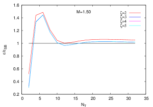
Figure 3: The $\zeta$ dependence of the energy density of domain wall fermions for $M=1.50$, $a_{5}=1$ and in the limit $N_{5}\rightarrow\infty$.

In order to highlight the deviations in the continuum limit, the same ratio is exhibited for different M values for $\zeta=4$ in Figure 4 as a function of $1/N_{T}^{2}$ and listed in Table 1 for a range of $N_{T}$ likely to be used in simulations. We choose to define the optimum range of M as the values of M for which the thermodynamic quantities are within 3% of the continuum values for the smallest possible $N_{T}$. One sees from both the Figure 4 and the Table 1 that the order $1/N_{T}^{2}$ corrections are minimum for M between 1.45-1.50 and $N_{T}\geq 12$.

Table 1: $\epsilon/\epsilon_{SB}$ values for different M for $\zeta=4$

$N_{T}$	M=1.0	1.40	1.45	1.50	1.55
4	0.909	1.240	1.286	1.333	1.384
6	1.308	1.413	1.426	1.444	1.469
8	1.317	1.221	1.197	1.175	1.159
10	1.236	1.090	1.051	1.009	0.966
12	1.168	1.048	1.011	0.966	0.915
14	1.123	1.043	1.014	0.977	0.930
16	1.092	1.046	1.026	0.998	0.960

The correction terms for $M=1$ are linear in $1/N_{T}^{2}$ for $N_{T}\geq 10$ and are about $20\%$ of the continuum value even for $N_{T}=12$. This is similar to that reported earlier for the overlap fermionsbgs . Though the continuum extrapolation with $M=1$ is easier due to the linear functional form, it is computationally expensive, needing simulations at more values of $N_{T}$, each greater than 10. Thus $M=$1.45-1.50 seems to be an optimum range for lattice simulation of the energy density of domain wall fermions. We have also varied the lattice spacing along the fifth dimension $a_{5}$ to find out how the cut-off dependent terms change with it. The correction terms to the energy density for $a_{5}=0.5$ at small lattice sizes $N_{T}\leq 10$ are indeed larger than that for $a_{5}=1$ for the above mentioned optimum range but for $N_{T}>12$ such terms are again within 2-3% of the Stefan Boltzmann value. The optimum $M$ range for which the lattice artifacts are minimum shifts to 1.50-1.60. Thus there is a marginal dependence on $a_{5}$ for $N_{T}\geq 10$. Reducing $a_{5}$ further does not increase the range much as we demonstrate in the plot for $a_{5}\rightarrow 0$ in Figure 6.

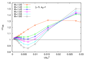
Figure 4: The variation of energy density of domain wall fermions with M in the limit $N_{5}\rightarrow\infty$ and $a_{5}=1$.

III.2 $N_{5}\rightarrow\infty~{},~{}a_{5}\rightarrow 0~{},~{}L_{5}=N_{5}a_{5}=\text{finite}$

Next we investigated the limit $N_{5}\rightarrow\infty~{},~{}a_{5}\rightarrow 0$ such that $L_{5}=N_{5}a_{5}=\text{finite}$ in order to estimate numerically the value of $L_{5}$ for which we recover the overlap energy density starting from Eq. (II.2). As can be observed from Figure 5, $L_{5}$-independent results are obtained for $L_{5}\geq 14$ for $M=1.55$. This was also the case for a range of $M$ around this value. For $L_{5}\leq 10$ the convergence towards the $\epsilon_{SB}$ value was seen to be very slow for all M and we find that the continuum value is not reached even for lattice size as large as $N_{T}=32$. Figure 6 displays the results as a function of $1/N_{T}^{2}$ for $L_{5}=14$ and various values of $M$ indicated on it. The deviations from the continuum for such $L_{5}$ are less than 3 % for the range of M between 1.50-1.60, in agreement with the overlap results bgs .

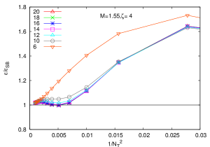
Figure 5: The variation of energy density on lattice with $N_{T}$ for domain wall fermions for different $L_{5}$, as shown by the respective labels, and $M=1.55$.

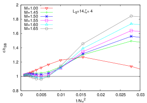
Figure 6: The variation of energy density on lattice with $1/N_{T}^{2}$ for domain wall fermions for $L_{5}=14$ and different M.

III.3 Finite $N_{5}$ and $a_{5}=1$

The case of finite $N_{5}$ with $a_{5}=1$ is clearly of most interest for practical simulations with dynamical fermions. Earlier numerical studies for free domain wall fermionsflem ; hegde employed $M=1.0$ and found somewhat slow convergence of various thermodynamic quantities towards their continuum values. We intend to check whether tuning the value of M results in a faster convergence. For that purpose we have computed the energy density expression for finite $N_{5}$ and $a_{5}=1$ in Eq.(II.3) by summing over all the discrete momenta. We display those results for $\epsilon/\epsilon_{SB}$ in Figure 7. The upper panel shows the results for a series of $N_{5}$ and a fixed $M=1.5$. The results are seen to become $N_{5}$-independent by $N_{5}=18$, making it an optimum choice for obtaining continuum results on the lattice. The lower panel shows the $M$-variation for $N_{5}=18$. Table 2 provides the values for lattices with reasonable $N_{T}$-extent. The general trend is clearly the same as above with $M=$1.45-1.50 emerging as the range for which the Stefan-Boltzmann limit is reached to within 3-4% for $N_{T}\geq 10$ (Table 2). Interestingly, $N_{5}=18$ seems to mimic the $N_{5}\rightarrow\infty$ limit quantitatively rather well as can be seen by comparing the Tables 1 and 2. Consequently, the same optimum range of $M$ is obtained for both.

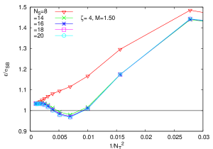
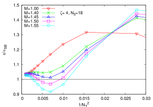
Figure 7: The variation of energy density on lattice with $1/N_{T}^{2}$ for domain wall fermions at different $N_{5}$ for $M=1.50$ (upper panel) and at $N_{5}=18$ for different $M$(lower panel).

Table 2: $\epsilon/\epsilon_{SB}$ values for different M for $\zeta=4,N_{5}=18$

$N_{T}$	M=1.0	1.40	1.45	1.50	1.55
4	0.909	1.240	1.285	1.333	1.383
6	1.308	1.413	1.425	1.443	1.467
8	1.317	1.221	1.197	1.174	1.156
10	1.237	1.090	1.052	1.009	0.965
12	1.169	1.049	1.013	0.968	0.917
14	1.123	1.045	1.017	0.980	0.934
16	1.093	1.048	1.029	1.002	0.966

IV Numerical results for $\hat{\mu}\neq 0$

It should be noted that in this case $T$ is no longer Hermitian but as long as the condition given in the Eq. (14) is satisfied the effective operator in Eq. (II.1) is well defined. We shall restrict the range of $\hat{\mu}$ to ensure that it is so. We choose $K$ and $L$ to be $e^{\pm\hat{\mu}}$ respectively in our numerical computations as suggested in wettig . Our aim again is to find the optimum $M$ for which the continuum results are obtained with least computational effort, and compare it with our the range obtained from the energy density above. We consider two observables here. One is the change in the energy density due to nonzero $\mu$ : $\Delta\epsilon(\mu,T)=\epsilon(\mu,T)-\epsilon(0,T)$. In the continuum limit this is

$$\frac{\Delta\epsilon(\mu,T)}{T^{4}}=\frac{\mu^{4}}{4\pi^{2}T^{4}}+\frac{\mu^{2}}{2T^{2}}.$$ (30)

Another observable we studied was the quark number susceptibility at $\hat{\mu}=0$. It is defined for any $\hat{\mu}$ by,

$$\chi=\frac{1}{N^{3}a^{2}N_{T}}\left(\frac{\partial^{2}\ln\det D}{\partial\hat{\mu}^{2}}\right)_{a_{4}}~{},~{}$$ (31)

and in the continuum is given by,

$$\chi(\mu)=\frac{\mu^{2}}{\pi^{2}}+\frac{T^{2}}{3}~{}.~{}$$ (32)

We will focus on $\chi(0)$ here due to its importance in the applications to the heavy ion collisions.

We estimated numerically $\Delta\epsilon(\mu,T)$ for $\mu/T=\hat{\mu}N_{T}$ fixed at 0.5. The upper and lower panels of the Figure 8 display our results for this observable in the units of $T^{4}$ for $N_{5}=\infty$ and 18 respectively for the $M$ values indicated. The horizontal line in each case shows the expected result in the continuum limit from Eq.(30). From the Figure 8 it is evident that there are no $\mu^{2}$ divergences on the lattice, as expected. The deviations from the continuum limit are due to the $M$ dependent finite size effects. These correction terms are again seen to be small for the same optimum range of $1.45\leq M\leq 1.50$ for both the cases, as obtained in the zero chemical potential case in section III.

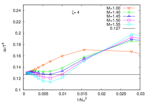
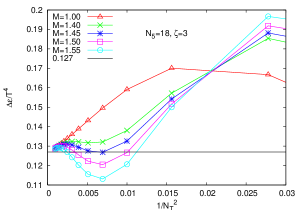
Figure 8: The energy density of domain wall fermions in presence of $\hat{\mu}$ for different $M$ for $\hat{\mu}=0.5/N_{T}$ and infinite $N_{5}$(upper panel) and for $N_{5}=18$ (lower panel).

The $N_{5}$ dependence of the quark number susceptibility at $\hat{\mu}=0$ is plotted in Figure 10. It too exhibits a convergence to the infinite $N_{5}$ results for $N_{5}\geq 16$, indicating that $N_{5}=18$ can again be used safely to approximate the infinite $N_{5}$. Figure 10 shows the $M$-dependence of the quark number susceptibility at $\hat{\mu}=0$. Both the $N_{5}=\infty$ (upper panel) and 18 (lower panel) show small deviations from the Stefan-Boltzmann value of $1/3$ for $1.45\leq M\leq 1.55$ range and for $N_{T}\geq 10$.

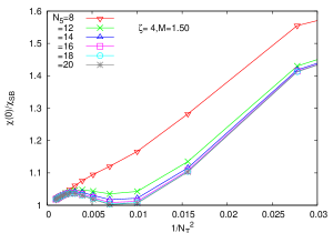
Figure 9: The quark number susceptibility as a function of $1/N_{T}^{2}$ for $N_{5}$ values as indicated for $M=1.5$ and $\zeta=4$.

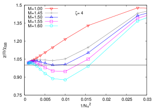
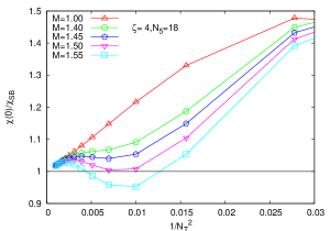
Figure 10: The quark number susceptibility as a function of $1/N_{T}^{2}$ for $M$ values as indicated for $\zeta=4$ and $N_{5}=\infty$ (upper panel) and 18 (lower panel).

Recent computations of this susceptibilityfks for the interacting domain wall fermions were performed with $M=1.8$. Of course, one expects some shift in $M$ due to the interactions, which should however be small for large enough temperature where one expects those computations to approach the free quark gas results. In all our plots we find that for the optimum $M$ range, the deviations from the ideal gas results at smaller $N_{T}=$4-8 are quite significant but with a relative mild $M$-dependence for $M>1.4$. Thus a slightly larger value of $M$ than the optimum range we found may not change the finite size effects drastically for small $N_{T}$. What one does need to be careful about though is the extrapolation to the continuum limit. For the optimal range of $M$ and $N_{T}\geq 10$, the smallness of corrections compared to other errors in the computations may make it a less important issue.

V Improvement of the chiral fermion kernels

In the previous sections we observed that the fermions with exact chiral symmetry on the lattice have large $1/N_{T}^{2}$ corrections for small $N_{T}$. While we found that the continuum limit for various thermodynamic quantities can be approached faster by choosing the irrelevant parameter $M$ in the range 1.45-1.55, the correction terms for $N_{T}=$4-6 are about twice that of the Stefan-Boltzmann result for such a choice of $M$ too. Here we describe our attempts to improve the convergence to the continuum results for small $N_{T}$ and even for $M=1.0$. Having the option of the choice of $M=1.0$ may be useful since it has been noted previouslyvranas ; cap that the residual mass for such a choice of $M$ is zero for a range of $N_{5}$ at the tree level.

V.1 Domain wall kernel

The domain wall operator given in Eq. (13) is a matrix-function of the Wilson-Dirac operator as in Eq. (II). It is clear that its improvement may lead to a better domain wall operator, or indeed even a better overlap operator, one is looking for. Inspired by the attempts to improve the staggered fermions in the so-called Naik-action naik , we add three-link terms to the $D_{W}$ as below.

$$D_{W}(x,x^{\prime},\hat{\mu})=\left(3+\frac{a}{a_{4}}-M\right)\delta_{x,x^{\prime}}-$$

$$\sum_{j=1}^{3}\left(U_{j}^{\dagger}(x-\hat{j})\frac{1+c_{1}\gamma_{j}}{2}\delta_{x,x^{\prime}+\hat{j}}+U_{j}(x)\frac{1-c_{1}\gamma_{j}}{2}\delta_{x,x^{\prime}-\hat{j}}\right)$$

$$- \frac{a}{a_{4}}\left(U_{4}^{\dagger}(x-\hat{4})\frac{1+c_{1}\gamma_{4}}{2}\delta_{x,x^{\prime}+\hat{4}}+U_{4}(x)\frac{1-c_{1}\gamma_{4}}{2}\delta_{x,x^{\prime}-\hat{4}}\right)$$

$$- \sum_{j=1}^{3}\left(U_{j}^{\dagger}(x-3\hat{j})\frac{c_{3}\gamma_{j}}{6}\delta_{x,x^{\prime}+3\hat{j}}-U_{j}(x)\frac{c_{3}\gamma_{j}}{6}\delta_{x,x^{\prime}-3\hat{j}}\right)$$

$$- \frac{a}{a_{4}}\left(U_{4}^{\dagger}(x-3_{\hat{4}})\frac{c_{3}\gamma_{4}}{6}\delta_{x,x^{\prime}+3_{\hat{4}}}-U_{4}(x)\frac{c_{3}\gamma_{4}}{6}\delta_{x,x^{\prime}-3_{\hat{4}}}\right)$$

Comparing with the Eq. (II), it is clear that the modification amounts to replacing $\gamma_{\mu}$ by $(c_{1}+c_{3}/3)\gamma_{\mu}$. The Wilson mass term, added to remove the doublers, is kept unchanged. Note that the modified $D_{W}$-operator is still $\gamma_{5}$-hermitian for arbitrary real values of the coefficients $c_{1}$ and $c_{3}$. The new domain wall operator can therefore be derived in the same way as Eq. (13) was obtained. We fix the coefficients by demanding the dispersion relation for free fermions on the lattice to be the same as in the the continuum up to $O(a^{4}p_{j}^{4})$. We find that all the terms at $O(a^{3}p_{j}^{3})$ are eliminated for the coefficients $c_{1}=9/8,~{}c_{3}=-1/8$. We employ them below for the calculation of the thermodynamic quantities.

The ratio of quark number susceptibilities, $\chi/\chi_{SB}$, computed using the above modified domain wall operator f1 , is plotted as a function of $1/N_{T}^{2}$ as in Figure 11 along with that for the unimproved domain wall operator of Eq. (13). We used $M=1$, $\zeta=4$, $N_{5}=18$ and $a_{5}=1$ for this computation. One clearly notices that the large correction terms ($\sim 45$%) at $N_{T}=$6-8 for the usual domain wall operator go down to about 7-8 %. Indeed, the size of corrections go down further as $N_{T}$ increases. Similarly, the the energy density of such improved fermions also exhibited smaller, about 15-5%, deviations from the continuum for $N_{T}=$6-10, as compared to about 30 % in the lower panel of Figure 7.

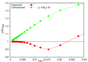
Figure 11: The susceptibility of improved and the conventional domain wall fermions at $M=1.0$ as a function of $1/N_{T}^{2}$.

V.2 Overlap kernel

From section II, we know that the overlap operator can be derived as a special limiting case of the domain wall operator. It would be thus interesting to check how the improvement in the Wilson Dirac operator in Eq. (V.1) fairs in the overlap case. For that purpose we compute the quark number susceptibility for non-interacting fermions on a $N^{3}\times N_{T}$ lattice numerically with the corresponding improved overlap operator. The $\chi/\chi_{SB}$ does have lower $1/N_{T}^{2}$ corrections for $N_{T}=6,8$ than for the conventional overlap operator with $M=1$ as shown in Figure 12. We also observe a faster approach to the continuum result with such improved overlap operator than with the Neuberger overlap operator even with optimum $M=1.55$ reported in bgs . Another advantage is that the thermodynamic quantities calculated from this improved operator are free from oscillations at odd-even values of $N_{T}$ exhibited bgs by the usual overlap operator. The improvement in the energy density is marginal up to $N_{T}=8$ but substantial for $N_{T}=10$ onwards.

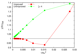
Figure 12: The $\chi/\chi_{SB}$ as a function of $1/N_{T}^{2}$ for the improved and the canonical overlap operators at $M=1.0$.

VI Conclusions & Discussions

Since the chiral violations vanish exponentially with the number of sites $N_{5}$ in the fifth dimension, the domain wall fermions offer a more practical alternative to the overlap fermions and yet have exact flavor and spin symmetry. We have computed the energy density and susceptibility at zero chemical potential of such fermions numerically for both finite and infinite $N_{5}$. The chiral symmetry is exact in the latter case and a choice $M$ between 1.45-1.50 allows faster convergence to the continuum results. We have also verified analytically that the energy density has the correct continuum value in the chiral limit. Varying the number of lattice sites in the fifth dimension, we have shown that $N_{5}=18$ is sufficient to restore chiral symmetry.

We found that introducing chemical potential $\hat{\mu}$ in domain wall operator leads to chiral symmetry breaking even for infinite $N_{5}$. But if we do allow that, there exist a large class of functions $K(\hat{\mu})$ and $L(\hat{\mu})$, with $K(\hat{\mu})\cdot L(\hat{\mu})=1$, for which there are no $\hat{\mu}$-dependent divergent terms in the physical observables. From the numerical evaluation of the energy density in presence of $\hat{\mu}$ , we conclude that the optimum range of $M$ remains the same. The lattice cut-off effects are however very large for small $N_{T}$ = 4-8. By systematically removing the dominant correction terms to the continuum value of the chiral fermion operators we have achieved a faster convergence to the continuum as well as small $1/N_{T}^{2}$ corrections for small lattice sizes even for $M=1.0$. This set of optimum parameters is anticipated to produce similar results in full QCD simulations with chiral fermions though an explicit check needs to be done.

Appendix A Proof for GW relation

We show here that the effective domain wall operator Eq. (15) satisfies the Ginsparg Wilson relation :

$$\gamma_{5}D_{DW} + D_{DW}\gamma_{5}=\gamma_{5}(1-\gamma_{5}\epsilon(\ln|T|))$$

$$+ (1-\gamma_{5}\epsilon(\ln|T|))\gamma_{5}$$

$$= 2~{}\gamma_{5}-\epsilon(\ln|T|)-\gamma_{5}\epsilon(\ln|T|)\gamma_{5}$$

$$D_{DW}\gamma_{5}D_{DW} = (1-\gamma_{5}\epsilon(\ln|T|))\gamma_{5}(1-\gamma_{5}\epsilon(\ln|T|))$$

$$= \gamma_{5}-\gamma_{5}\epsilon(\ln|T|)\gamma_{5}-\epsilon(\ln|T|)+\gamma_{5}\epsilon^{2}(\ln|T|)$$

Since,

$$\epsilon(\ln|T|) = \frac{\ln|T|}{\sqrt{(\ln|T|)\ln|T|}}$$

$$\therefore\epsilon^{2}(\ln|T|) = \frac{\ln|T|\ln|T|}{(\sqrt{\ln|T|\ln|T|})^{2}}=1$$ (34)

Hence $\{\gamma_{5},D_{DW}\}=D_{DW}\gamma_{5}D_{DW}$

References

- (1) D. B. Kaplan, Phys. Lett. B288, 342 (1992).
- (2) P. M. Vranas, Phys. Rev. D57, 1415 (1998).
- (3) Y. Shamir, Nucl. Phys. B406, 90 (1993).
- (4) J. Bloch and T. Wettig, Phys. Rev. D76, 114511 (2007).
- (5) R. V. Gavai, Phys. Rev. D32, 519 (1985).
- (6) H. Neuberger, Phys. Rev. D57, 5417 (1998).
- (7) R. G. Edwards and U. M. Heller, Phys. Rev. D63, 094505 (2001).
- (8) R. Narayanan and H. Neuberger, Phys. Rev. Lett. 71, 3251 (1993); H. Neuberger, Phys. Lett. 417B, 141 (1998).
- (9) P. H. Ginsparg and K. G. Wilson, Phys. Rev. D25, 2649 (1982).
- (10) M. Luscher, Phys. Lett. B428, 342 (1998).
- (11) D. Banerjee, R. V. Gavai and S. Sharma, Phys. Rev. D78, 014506 (2008).
- (12) R. V. Gavai and S. Sharma, J. Phys. G 35, 104097 (2008).
- (13) G. T. Flemming, Nucl. Phys. Proc. Suppl. 94, 393 (2001).
- (14) P. Hegde et al., Eur. Phys. J. , C55, 423 (2008).
- (15) P. Hasenfratz and F. Karsch, Phys. Lett. 125B, 308 (1983).
- (16) P. Hegde, F. Karsch and C. Schmidt, e-Print arxiv:0810.0290[hep-lat].
- (17) S. Capitani, Phys. Rev. D75, 054505 (2007).
- (18) S. Naik, Nucl. Phys. B316, 238 (1989).
- (19) Following gavlat , we use and for introducing for the 3-link terms.
- (20) R. V. Gavai, Nucl. Phys. Proc. Suppl. 119, 529 (2003).