Bounds on Rayleigh-Bénard convection with imperfectly conducting plates

Abstract

We investigate the influence of the thermal properties of the boundaries in turbulent Rayleigh-Bénard convection on analytical upper bounds on convective heat transport. We model imperfectly conducting bounding plates in two ways: using idealized mixed thermal boundary conditions of constant Biot number $\eta$, continuously interpolating between the previously studied fixed temperature ($\eta=0$) and fixed flux ($\eta=\infty$) cases; and by explicitly coupling the evolution equations in the fluid in the Boussinesq approximation through temperature and flux continuity to identical upper and lower conducting plates. In both cases, we systematically formulate a bounding principle and obtain explicit upper bounds on the Nusselt number $\mathit{Nu}$ in terms of the usual Rayleigh number $\mathit{Ra}$ measuring the average temperature drop across the fluid layer, using the “background method” developed by Doering and Constantin. In the presence of plates, we find that the bounds depend on $\sigma=d/\lambda$, where $d$ is the ratio of plate to fluid thickness and $\lambda$ is the conductivity ratio, and that the bounding problem may be mapped onto that for Biot number $\eta=\sigma$. In particular, for each $\sigma>0$, for sufficiently large $\mathit{Ra}$ (depending on $\sigma$) we show that $\mathit{Nu}\leq c(\sigma)R^{1/3}\leq C\mathit{Ra}^{1/2}$, where $C$ is a $\sigma$-independent constant, and where the control parameter $R$ is a Rayleigh number defined in terms of the full temperature drop across the entire plate-fluid-plate system. In the $\mathit{Ra}\to\infty$ limit, the usual fixed temperature assumption is a singular limit of the general bounding problem, while fixed flux conditions appear most relevant to the asymptotic $\mathit{Nu}$–$\mathit{Ra}$ scaling even for highly conducting plates.

1 Introduction

The Rayleigh-Bénard system, in which a fluid layer between two parallel plates is heated from below, is a popular model system for the experimental and theoretical investigation of the important phenomenon of convection, in which density changes due to heating give rise to buoyancy-driven fluid flow (Normand et al. (1977); Kadanoff (2001); Cross & Hohenberg (1993)). With sufficient heating the flow becomes turbulent, and the spatiotemporal dynamics become inaccessible to a detailed analytical or experimental understanding; instead, one focusses on bulk statistical properties. Of considerable interest is the dimensionless Nusselt number $\mathit{Nu}$, which measures the averaged total heat flux relative to what it would be in the absence of convection, since the convective fluid motion transports heat upward more efficiently than would be achieved by pure conduction with the same overall temperature gradient.

In particular, much research has concentrated on trying to understand the dependence of $\mathit{Nu}$ on the (averaged) temperature difference across the plates, represented in nondimensional form by the Rayleigh number $\mathit{Ra}$, which measures the relative strength of buoyancy and dissipative forces. This dependence is often assumed to take the power law form (with possible logarithmic corrections) $\mathit{Nu}\sim C\mathit{Ra}^{p}$. Here the prefactor $C$ may depend on the geometry of the experimental apparatus (for instance, the aspect ratio of a typical cylindrical cell) and/or the Prandtl number $\mathit{Pr}$.

In spite of numerous studies over the years, a consensus on the precise form of this scaling relationship (especially in the large-$\mathit{Ra}$ limit) remains elusive. Experiments have typically found the exponent $p$ to lie in the range $1/4$–$1/3$ (see for instance Heslot et al. (1987); Glazier et al. (1999); Niemela & Sreenivasan (2006b); Funfschilling et al. (2009), or the reviews by Kadanoff (2001), Procaccia & Sreenivasan (2008) and Ahlers et al. (2009b)), although higher values have also been reported (Chavanne et al. (2001)). Phenomenological models have also made various predictions, ranging from the early values $p=1/3$ (Malkus (1954)) and $p=1/2$ (Kraichnan (1962)), both supported by dimensional arguments, to a more recent model due to Grossmann & Lohse (2000), which predicts different superpositions of scaling exponents in different parameter regimes. Meanwhile, the numerical investigations of Amati et al. (2005) in cylindrical geometry (performed at higher resolution by Stevens et al. (2010)) found the scaling $p=1/3$ (though, surprisingly, the recent two-dimensional, horizontally periodic computations of Johnston & Doering (2009) are consistent with $p=2/7$).

Effect of imperfectly conducting plates bounding the fluid:

While some of the variations in the observed results and discrepancies between experiment and theory may be due to sidewall conductivity, Prandtl number variability, non-Boussinesq effects, geometry or other factors, recent attention has increasingly focussed on the influence of the thermal properties of the fluid boundaries. The standard assumption for Rayleigh-Bénard convection is that the upper and lower boundaries of the fluid are held at uniform and fixed temperature; this is equivalent to the bounding plates being perfectly conducting. In experimental situations, however, the thermal conductivity $\lambda_{s}$ of the plates is finite, though typically much larger than the conductivity $\lambda_{f}$ of the fluid. In the convective state, the rate at which the fluid transports heat is effectively comparable to that which would ensue from conduction with conductivity $\mathit{Nu}\,\lambda_{f}$. Hence, for sufficiently strong heating, the assumption that the plates transport heat much more efficiently than the fluid, and are able to maintain the fluid boundaries at constant temperature, loses validity; indeed, in the asymptotic high-$\mathit{Ra}$ limit, one might expect that relative to the fluid, the plates are effectively insulating.

A basic consideration in investigating the influence of poorly conducting boundaries on convection is the choice of thermal boundary conditions (BCs). Numerous researchers have concentrated solely on idealized fixed flux conditions corresponding to perfectly insulating boundaries (for instance Chapman & Proctor (1980); Otero et al. (2002); Verzicco & Sreenivasan (2008); Johnston & Doering (2009)), while other studies (including Sparrow et al. (1964); Gertsberg & Sivashinsky (1981); Westerburg & Busse (2001)) have imposed more general mixed conditions of fixed Biot number $\eta$ at the fluid boundaries. Note, though, that the Biot number in general depends on the horizontal “disturbance” wave number in the plates (Normand et al., 1977, Section V.C.1). For strong driving (high $\mathit{Ra}$), the temperature distribution in the plates is unsteady and contains a superposition of horizontal wave numbers, so that even mixed, fixed $\eta$ conditions form an approximation to the experimentally more realistic situation of a fluid bounded by plates of finite width and conductivity. Consequently, some authors have studied the effect of imperfectly conducting boundaries by directly incorporating plates in their models, for the study of both the convective instability and the weakly nonlinear behaviour beyond transition (for instance Hurle et al. (1967); Proctor (1981); Jenkins & Proctor (1984); Holmedal et al. (2005)) and for high-$\mathit{Ra}$ convective turbulence (Chillà et al. (2004); Verzicco (2004)).

The influence of the plate thermal properties on the initial instability of the conductive state and the weakly nonlinear dynamics and pattern formation beyond instability has been studied intensively since the pioneering works of Sparrow et al. (1964); Hurle et al. (1967); Busse & Riahi (1980); Chapman & Proctor (1980) and others. Their effect on heat transport in turbulent convection has, however, only been considered much more recently, though it is now receiving attention in the context of experiments, numerical computation, phenomenological modelling and rigorous analysis. In the latter category is the study by Otero et al. (2002), who considered analytical bounds for fixed flux convection (perfectly insulating boundaries), as discussed further below.

The suggestion that the finite (even if large) heat capacity and conductivity of the plates would affect heat transport was made by Chaumat et al. (2002), who subsequently extended their phenomenological model to propose a criterion for sufficient ideality of the plates’ thermal properties for the Kraichnan $p=1/2$ “ultimate regime” to develop (Chillà et al. (2004); see also Roche et al. (2005)); while Hunt et al. (2003) modelled the effect of the thermal diffusivity of the lower plate on plume formation and eddy motion. On the basis of extensive numerical studies with varying plate properties Verzicco (2004) concluded that the effects of the plates are governed by the ratio of the thermal resistance of the fluid layer to that of the plates, and proposed a model quantifying the resultant effect on the Nusselt number, which was partially confirmed in experiments by Brown et al. (2005); see also Niemela & Sreenivasan (2006a) and Ahlers et al. (2009a).

The role of boundary thermal properties is also receiving increasing attention in the geophysical community in the context of heat transport due to mantle convection. The ocean floor and continents impose different thermal conditions at the upper boundary of the Earth’s mantle: the oceans are well-described as enforcing a fixed temperature, while continents act as (partial) insulators, and are modelled as lids of finite conductivity fully or partially covering the convecting fluid. The presence of continents is understood to affect the convective flow (Guillou & Jaupart (1995)), and the effect of finitely conducting continents on heat transport in mantle convection has been investigated through models and numerical simulations (Lenardic & Moresi (2003); Grigné et al. (2007a, b)).

Careful numerical investigations permit control of extraneous variables that may play a role experimentally, thus making it possible to isolate the effect of the thermal boundary conditions. Two groups have recently explored this independently: the two-dimensional, horizontally periodic computations of Johnston & Doering (2009) studied fixed temperature and fixed flux BCs both above and below, while Verzicco & Sreenivasan (2008) and Stevens et al. (2010) compared the effects of fixed flux and fixed temperature lower horizontal plates in their cylindrical simulations. No differences between the extremes of perfectly conducting and insulating boundaries were observed in either case. However, direct numerical simulations are as yet unable to attain the high Rayleigh numbers achieved experimentally or relevant to, for instance, geophysical or astrophysical applications.

Analytical upper bounds on convective heat transport:

In the investigation of transport and scaling properties, mathematical results systematically derived from the differential equations governing the system can play a role. The details of turbulent dynamics are beyond the reach of analysis, but bounds on averaged quantities can often be obtained, and provide constraints against which phenomenological theories can be tested, and which are in many situations (though not so far in finite Prandtl number convection) remarkably close to experimental observation. In the case of Rayleigh-Bénard convection with fixed temperature BCs, a bound of the form $\mathit{Nu}\leq C_{0}\mathit{Ra}^{1/2}$ has been shown, initially with the aid of some plausible statistical assumptions (Howard (1963); Busse (1969)). More recently, the “background method” introduced in the context of shear flow by Doering & Constantin (1992), motivated by a decomposition due to Hopf (1941), has enabled the above $p=1/2$ bound to be proved rigorously without any additional assumptions (Doering & Constantin (1996)). This approach has turned out to be remarkably fruitful; its applications to convection have included, among others, studies of porous medium (Otero et al. (2004)), infinite Prandtl number (Doering et al. (2006)), and double diffusive (Balmforth et al. (2006)) convection.

The first investigation to consider the effects of thermal boundary conditions on rigorous variational bounds on convective heat transport was that of Otero et al. (2002), who considered upper and lower fixed flux BCs. This work established an overall bound of the form $\mathit{Nu}\leq C_{\infty}\mathit{Ra}^{1/2}$, with the same scaling as in the fixed temperature case; but the mathematical structure of the bounding calculations and the intermediate scaling results in the two cases turned out to be quite different. When the temperature drop across the fluid is fixed, the Rayleigh number $\mathit{Ra}$ is the control parameter, and one obtains bounds on the heat transport by controlling the averaged heat flux through the fluid boundaries from above (Doering & Constantin (1996); Kerswell (2001)). On the other hand, given a fixed boundary heat flux, the control parameter $R$ is defined in terms of this imposed flux; in this case the averaged temperature difference between the fluid boundaries (and hence the Rayleigh number $\mathit{Ra}$) must be estimated (from below) in terms of $R$ to find bounds on $\mathit{Nu}$. One finds (Otero et al. (2002)) that $\mathit{Nu}\leq c_{1}R^{1/3}$, $\mathit{Ra}\geq c_{2}R^{2/3}$, unlike in the fixed temperature case for which $\mathit{Nu}\leq C_{0}R^{1/2}$, $\mathit{Ra}=R$. It is thus natural to wonder how these two extreme cases, corresponding respectively to the idealizations of perfectly conducting and insulating plates, are related vis-à-vis their bounding problems, and which is more relevant to real, finitely conducting boundaries.

Outline of this paper:

In the present work we reconsider the effect of general thermal BCs on systematically derived analytical bounds on thermal convection, continuing the program initiated by Otero et al. (2002); we assume for simplicity only identical thermal properties at the top and bottom fluid boundaries in the mathematically idealized horizontally periodic case.

We model imperfectly conducting plates in two different ways. One method is to assume mixed (Robin) thermal BCs of “Newton’s Law of Heating” type, with a fixed Biot number $\eta$, and to develop the analysis in a manner which interpolates smoothly between the fixed temperature (Dirichlet: $\eta=0$) and fixed flux (Neumann: $\eta=\infty$) extremes (to our knowledge the only prior bounding study with general Biot number is the horizontal convection work of Siggers et al. (2004), with mixed BCs at the lower boundary). The other approach is to consider the more realistic case of a fluid in thermal contact above and below with finite conducting plates, restricting ourselves to homogeneous, isotropic plates with fixed temperatures imposed at the top and bottom of the entire system.

In § 2 we formulate the governing equations for Rayleigh-Bénard convection and discuss various thermal BCs, paying particular attention to the choice of nondimensionalization. Global identities and averages, including energy identities for convection with plates, are discussed in § 3, while a bounding principle using the Constantin-Doering-Hopf “background field” variational method is derived in § 4. The use of a piecewise linear background temperature profile and of conservative estimates in § 5 permits the derivation of explicit analytical bounds on the $\mathit{Nu}$-$\mathit{Ra}$ relationship, asymptotically valid as $\mathit{Ra}\to\infty$, as discussed in § 6. For clarity, §§ 3.2–5.1 of the main text treat the case of convection with plates, while the corresponding calculations for fixed Biot number BCs are presented in a parallel fashion in Appendix B.

Summary of results:

For convection with plates, we find that the heat transport depends on $d$, the ratio of plate to fluid thickness, and $\lambda$, the conductivity ratio, only via the combination $\sigma=d/\lambda$; and that the (conservative) bounding problems with plates and with fixed Biot number $\eta$ map onto each other when $\sigma=\eta$; this gives a systematic correspondence between the “full” problem of conducting plates and the fixed Biot number approximation, without stationarity, fixed horizontal wave number or other modelling assumptions.

Since in general the boundary temperatures are unknown a priori, one must identify a temperature scale $\Theta$ extracted from the thermal BCs; a control parameter $R$, defined like a Rayleigh number but in terms of $\Theta$, may then be introduced as a measure of the applied driving. For sufficiently small Biot number $\eta$ (or, equivalently, $\sigma$), we show that for small $R$ we have $\mathit{Nu}\lesssim{\mathcal{O}}(R^{1/2})$, $\mathit{Ra}\gtrsim{\mathcal{O}}(R)$ as in the fixed temperature case, but that for $R$ (and hence $\mathit{Ra}$) beyond some critical parameter which we estimate as $R_{\mathrm{t}}={\mathcal{O}}(\eta^{-2})$, we find $\mathit{Nu}\leq c_{1}(\eta)R^{1/3}$, $\mathit{Ra}\geq c_{2}(\eta)R^{2/3}$, implying $\mathit{Nu}\leq C_{\eta}\mathit{Ra}^{1/2}$ with intermediate scaling as in the fixed flux case. Interestingly, for each $\eta>0$ we find $C_{\eta}=C_{\infty}$: at least at the level of our estimates, the asymptotic scaling in each case is as for fixed flux BCs, while fixed temperature BCs give a singular limit of the general asymptotic bounding problem.

Interpreted in terms of convection with plates, the analytical bounds on the $\mathit{Nu}$–$\mathit{Ra}$ relationship confirm that for relatively small $R$ most of the temperature drop occurs across the fluid. However, for each $\sigma>0$, asymptotically as $R\to\infty$ we have $\mathit{Nu}\leq c(\sigma)R^{1/3}\leq C_{\infty}\mathit{Ra}^{1/2}$: the bounds scale as in the fixed flux case, providing rigorous support for the intuition that for large $\mathit{Ra}$, plates of arbitrary finite thickness and conductivity act essentially as insulators. The asymptotic result $\mathit{Nu}\leq c(\sigma)R^{1/3}$, where $c(\sigma)={\mathcal{O}}(\sigma^{-1/3}(1+2\sigma)^{1/3})$ is of particular interest, since in this case $R$ may be interpreted as a Rayleigh number in terms of the full temperature difference across the entire system.

2 Governing equations and thermal boundary conditions

2.1 Governing differential equations and nondimensionalization

We consider a fluid of depth $h$, kinematic viscosity $\nu_{f}$ and thermal diffusivity $\kappa_{f}$, with density $\rho_{f}$ at some reference temperature $T_{0}$; we also let $\alpha$ be the thermal expansion coefficient, $c_{p,f}$ be the specific heat and hence $\lambda_{f}=\rho_{f}\,c_{p,f}\,\kappa_{f}$ be the thermal conductivity of the fluid.

The (dimensional) partial differential equations (PDEs) of motion in the Boussinesq approximation, describing the evolution of the fluid velocity field $\mathbf{u}^{*}$ and temperature field $T^{*}$, are

$$\frac{\partial\mathbf{u}^{*}}{\partial t^{*}}+\mathbf{u}^{*}\cdot\mbox{\boldmath$\nabla$\unboldmath}^{*}\mathbf{u}^{*}+\frac{1}{\rho_{f}}\mbox{\boldmath$\nabla$\unboldmath}^{*}P^{*} =\nu_{f}\nabla^{*2}\mathbf{u}^{*}+\alpha g(T^{*}-T_{0})\,{\bf e_{z}}\ ,$$ (2.1)

$$\mbox{\boldmath$\nabla$\unboldmath}^{*}\cdot\mathbf{u}^{*} =0\ ,$$ (2.2)

$$\frac{\partial T^{*}}{\partial t^{*}}+\mathbf{u}^{*}\cdot\mbox{\boldmath$\nabla$\unboldmath}^{*}T^{*} =\kappa_{f}\nabla^{*2}T^{*}\$$ (2.3)

(where $g$ is the gravitational acceleration). In this formulation, the compressibility of the fluid is neglected everywhere except in the buoyancy force term, and the pressure $P^{*}$ is determined via the divergence-free condition on $\mathbf{u}^{*}$. Variables with an asterisk are dimensional, and we take periodic boundary conditions in the horizontal directions, with periods $L^{*}_{x}$ and $L^{*}_{y}$, respectively. In the vertical direction, the fluid satisfies no-slip velocity boundary conditions $\mathbf{u}^{*}=\mathbf{0}$ at $z^{*}=0$ and $z^{*}=h$.

The nondimensionalization is chosen to treat the different thermal boundary conditions (BCs) at the interfaces between the fluid and the plates at $z^{*}=0$, $h$ consistently and in a single formulation. For now, we thus let $\Theta$ be a general temperature scale, and introduce a reference (“zero”) temperature $T_{\text{ref}}$; for given thermal BCs, the approach which turns out to be successful is to define $\Theta$ and $T_{\text{ref}}$ so that the stationary, horizontally uniform perfectly conducting state in the fluid ($\mathbf{u}^{*}=\mathbf{0}$, $\mbox{\boldmath$\nabla$\unboldmath}^{*}T^{*}=C\,{\bf e_{z}}$ for some constant $C<0$) takes the nondimensional form

$$\mathbf{u}=\mathbf{0},\quad T=1-z\qquad(0<z<1).$$ (2.4)

We nondimensionalize using $T_{\text{ref}}$ and the temperature scale $\Theta$, and with respect to the fluid layer thickness $h$ and thermal diffusivity time $h^{2}/\kappa_{f}$; that is, we take $h$, $h^{2}/\kappa_{f}$, $U=\kappa_{f}/h$ and $\rho_{f}U^{2}$ as our appropriate length, time, velocity and pressure scales respectively. For $T_{\text{ref}}\not=T_{0}$, the nondimensional fluid momentum equation will contain a constant term proportional to $T_{\text{ref}}-T_{0}$ in the ${\bf e_{z}}$ direction, which we absorb into the rescaled pressure. In summary, the nondimensional variables (without asterisks) are defined by:

$$\mathbf{x}=\frac{\mathbf{x}^{*}}{h},\quad t=\frac{t^{*}}{t_{\text{scal}}},\quad\mathbf{u}=\frac{\mathbf{u}^{*}}{U},\quad T=\frac{T^{*}-T_{\text{ref}}}{\Theta},\quad p=\frac{1}{\mathit{Pr}}\frac{P}{\rho_{f}U^{2}}-R\frac{T_{\text{ref}}-T_{0}}{\Theta}z,$$ (2.5)

where $t_{\text{scal}}=h^{2}/\kappa_{f}$, $U=\kappa_{f}/h$, and $\mathit{Pr}$ and $R$ are defined below. The dimensionless periodicity lengths in the transverse directions are $L_{x}=L^{*}_{x}/h$ and $L_{y}=L^{*}_{y}/h$, and $A=L_{x}L_{y}$ is the nondimensional area of the plates.

The equations for the nondimensional fluid velocity $\mathbf{u}=(u,v,w)$ and fluid temperature $T$ are thus

$$\mathit{Pr}^{-1}\left(\frac{\partial\mathbf{u}}{\partial t}+\mathbf{u}\cdot\mbox{\boldmath$\nabla$\unboldmath}\mathbf{u}\right)+\mbox{\boldmath$\nabla$\unboldmath}p =\nabla^{2}\mathbf{u}+R\,T\,{\bf e_{z}},$$ (2.6)

$$\mbox{\boldmath$\nabla$\unboldmath}\cdot\mathbf{u} =0,$$ (2.7)

$$\frac{\partial T}{\partial t}+\mathbf{u}\cdot\mbox{\boldmath$\nabla$\unboldmath}T =\nabla^{2}T,$$ (2.8)

with no-slip BCs $\mathbf{u}|_{z=0,1}=\mathbf{0}$, and $L_{x},\ L_{y}$-periodic BCs in the horizontal $x$ and $y$ directions in all variables.

Here the dimensionless constants are the usual Prandtl number $\mathit{Pr}=\nu_{f}/\kappa_{f}$ and the control parameter $R$, defined in terms of the (as yet unspecified) temperature scale $\Theta$ as

$$R=\frac{\alpha gh^{3}}{\nu_{f}\kappa_{f}}\,\Theta\ .$$ (2.9)

2.2 Thermal boundary conditions imposed at interfaces

The specification of the governing equations is completed once conditions on the temperature at the fluid-plate interfaces $z^{*}=0$ and $z^{*}=h$ are specified. We shall consider both thermal BCs applied directly at these interfaces, as in figure 1, and (in § 2.3 below) the case of solid plates in thermal contact with the fluid; in each case we restrict ourselves to fluids with thermally identical upper and lower boundaries.

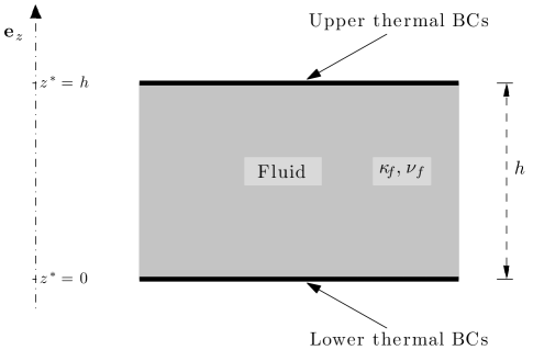
Figure 1: Geometry of Rayleigh-Bénard convection system with thermal boundary conditions imposed at upper and lower limits of fluid layer.

Fixed temperature (Dirichlet) conditions:

The usual and most-studied assumption regarding thermal boundary conditions at the interfaces is that the temperature is fixed at the upper and lower fluid boundaries:

$$T^{*}|_{z^{*}=0}\equiv T^{*}(x^{*},y^{*},0,t^{*})=T_{b}^{*},\qquad T^{*}|_{z^{*}=h}=T_{t}^{*}.$$ (2.10)

These Dirichlet BCs imply a natural choice of reference temperature $T_{\text{ref}}=T_{t}^{*}$, while the imposed temperature drop $\Delta T^{*}\equiv-\left.T^{*}\right|_{z^{*}=0}^{h}\equiv T_{b}^{*}-T_{t}^{*}$ introduces a natural temperature scale $\Theta=\Delta T^{*}$. The nondimensional thermal BCs thus take the well-known form

$$T=1\ \ \text{on}\ \ z=0,\qquad T=0\ \ \text{on}\ \ z=1.$$ (2.11)

Fixed flux (Neumann) conditions:

At the opposite extreme is the fixed flux assumption that the thermal heat flux $-\lambda_{f}T^{*}_{z^{*}}\equiv-\lambda_{f}\,\partial T^{*}/\partial z^{*}$ through the fluid boundaries is a constant $\Phi$. This corresponds to the Neumann BCs of fixed normal temperature gradient $-\beta^{*}$ at the interfaces:

$$T^{*}_{z^{*}}|_{z^{*}=0}=T^{*}_{z^{*}}|_{z^{*}=h}=-\beta^{*}=-\frac{\Phi}{\lambda_{f}};$$ (2.12)

the corresponding temperature scale is $\Theta=h\beta^{*}=h\Phi/\lambda_{f}$, while in this case $T_{\text{ref}}$ is arbitrary. In this limit, the dimensionless thermal BCs are

$$T_{z}=-1\ \ \text{on}\ \ z=0\ \text{and}\ z=1.$$ (2.13)

Fixed Biot number (Robin) conditions:

General linear thermal conditions at the boundary of a fluid as in figure 1 are of mixed (Robin) type; in dimensional terms, we write the mixed BCs in the form

$$T^{*}+\eta^{*}{\bf n}\cdot\mbox{\boldmath$\nabla$\unboldmath}^{*}T^{*}=A_{l}^{*}\ \ \text{on}\ \ z^{*}=0,\qquad T^{*}+\eta^{*}{\bf n}\cdot\mbox{\boldmath$\nabla$\unboldmath}^{*}T^{*}=A_{u}^{*}\ \ \text{on}\ \ z^{*}=h.$$ (2.14)

for some given constant $0\leq\eta^{*}<\infty$. These conditions may be interpreted as Newton’s Law of Cooling (Heating), in which the boundary heat flux is assumed proportional to the temperature change across the boundary: $-\lambda_{f}{\bf n}\cdot\mbox{\boldmath$\nabla$\unboldmath}^{*}T^{*}=\lambda_{f}(T^{*}-A_{l}^{*})/\eta^{*}$.

We use ${\bf n}=-{\bf e_{z}},+{\bf e_{z}}$ on $z^{*}=0,h$ respectively, and nondimensionalize by substituting $z^{*}=hz$, $T^{*}=T_{\text{ref}}+\Theta T$. Defining the Biot number $\eta=\eta^{*}/h$, we find

$$T-\eta\,T_{z}=\frac{A_{l}^{*}-T_{\text{ref}}}{\Theta}\ \ \text{on}\ \ z=0,\qquad T+\eta\,T_{z}=\frac{A_{u}^{*}-T_{\text{ref}}}{\Theta}\ \ \text{on}\ \ z=1.$$ (2.15)

The so far unspecified reference temperature $T_{\text{ref}}$ and temperature scale $\Theta$ are now determined by the condition (2.4) on the nondimensional form of the conduction temperature profile: requiring $T=1-z$ to satisfy the BCs (2.15), we find that (for $\eta<\infty$)

$$\Theta=\frac{A_{l}^{*}-A_{u}^{*}}{1+2\eta},\qquad T_{\text{ref}}=\frac{A_{u}^{*}+\eta(A_{l}^{*}+A_{u}^{*})}{1+2\eta}.$$ (2.16)

Having finally fixed a choice of dimensionless variables, the nondimensional mixed thermal boundary conditions (fixed Biot number) are

$$T-\eta\,T_{z}=1+\eta\ \ \text{on}\ \ z=0,\qquad T+\eta\,T_{z}=-\eta\ \ \text{on}\ \ z=1.$$ (2.17)

Note that the mixed (Robin) BCs (2.17) reduce to the fixed temperature (Dirichlet) BCs (2.11) in the limit $\eta\to 0$, and to the fixed flux (Neumann) BCs (2.13) in the limit $\eta\to\infty$; thus we denote $\eta=0$ and $\eta=\infty$ as the “fixed temperature” and “fixed flux” cases, respectively.

2.3 Fluid bounded by conducting plates

The specification of thermal conditions directly at the fluid boundaries $z^{*}=0$, $h$, as in § 2.2, is an approximation to the experimentally more realistic situation of a fluid bounded above and below by conducting plates, with thermal BCs imposed on the plates. We consider only the simplest case of plates with equal thickness and thermal properties.

Beginning with a fluid with properties as in § 2.1, we thus place identical homogeneous, isotropic solid plates of thickness $h_{s}$, thermal diffusivity $\kappa_{s}$ and thermal conductivity $\lambda_{s}=\rho_{s}\,c_{p,s}\,\kappa_{s}$ above and below the fluid; see figure 2.

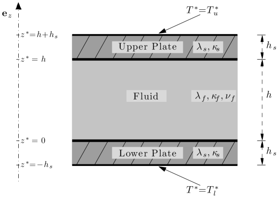
Figure 2: Geometry of Rayleigh-Bénard convection system with conductive plates.

The spatial coordinates are chosen so that $z^{*}=0$ is at the lower boundary of the fluid, and thus the lower and upper plates extend from $z^{*}=-h_{s}$ to $z^{*}=0$, and from $z^{*}=h$ to $z^{*}=h+h_{s}$, respectively.

The governing PDEs in the fluid in the Boussinesq approximation, valid in the region $0<z^{*}<h$, are as in (2.1)–(2.3) above, where $T^{*}=T^{*}_{f}$ is the fluid temperature field, and the fluid velocity $\mathbf{u}^{*}$ satisfies the usual no-slip boundary conditions at $z^{*}=0$ and $z^{*}=h$, the interfaces between the fluid and the plates.

These equations are coupled to the heat equation for the temperature $T^{*}_{p}$ in the plates,

$$\frac{\partial T^{*}_{p}}{\partial t^{*}}=\kappa_{s}\mbox{\boldmath$\nabla$\unboldmath}^{*2}T^{*}_{p},$$ (2.18)

valid in the lower plate for $-h_{s}<z^{*}<0$ and in the upper plate for $h<z^{*}<h+h_{s}$.

At the interfaces (where ${\bf n}={\bf e_{z}}$) we require continuity of temperature $T^{*}$ and normal heat flux $\lambda\,{\bf n}\cdot\mbox{\boldmath$\nabla$\unboldmath}T^{*}=\lambda\,\partial T^{*}/\partial z^{*}$. With $T^{*}_{f}$, $T^{*}_{p,l}$ and $T^{*}_{p,u}$ representing the (dimensional) temperature in the fluid, lower plate and upper plate, respectively (letting subscripts $l$ and $u$ identify the plates), continuity of temperature may be written as

$$T^{*}_{p,l}|_{z^{*}=0}=T^{*}_{f}|_{z^{*}=0}\ ,\qquad T^{*}_{f}|_{z^{*}=h}=T^{*}_{p,u}|_{z^{*}=h}\ ,$$

and similarly for flux continuity. However, it is more convenient to treat $T^{*}$ as a single temperature field, continuous but with discontinuous derivative, which coincides with $T^{*}_{p,l}$ for $-h_{s}\leq z^{*}<0$, with $T^{*}_{f}$ for $0<z^{*}<h$, and with $T^{*}_{p,u}$ for $h<z^{*}\leq h+h_{s}$; and we write, for instance, $T^{*}|_{z^{*}=0+}=\lim_{z^{*}\to 0+}T^{*}=T^{*}_{f}|_{z^{*}=0}$, or $(\partial T^{*}/\partial z^{*})|_{z^{*}=0-}=(\partial T^{*}_{p,l}/\partial z^{*})|_{z^{*}=0}$ (see Appendix A concerning notation). We may then express the continuity of temperature and heat flux at the fluid-plate interfaces as: for each $x^{*}$, $y^{*}$ and $t^{*}$,

$$T^{*}|_{z^{*}=0-}=T^{*}|_{z^{*}=0+}\ ,\qquad T^{*}|_{z^{*}=h-}=T^{*}|_{z^{*}=h+}\ ,$$ (2.19)

and

$$\left.\lambda_{s}\frac{\partial T^{*}}{\partial z^{*}}\right|_{z^{*}=0-}=\left.\lambda_{f}\frac{\partial T^{*}}{\partial z^{*}}\right|_{z^{*}=0+},\qquad\left.\lambda_{f}\frac{\partial T^{*}}{\partial z^{*}}\right|_{z^{*}=h-}=\left.\lambda_{s}\frac{\partial T^{*}}{\partial z^{*}}\right|_{z^{*}=h+}.$$ (2.20)

We assume that the entire plate-fluid-plate system has Dirichlet thermal boundary conditions in the vertical direction (in addition to horizontal periodicity in all variables), with fixed temperatures at the bottom of the lower plate and the top of the upper plate,

$$T^{*}|_{z^{*}=-h_{s}}=T_{l}^{*},\qquad T^{*}|_{z^{*}=h+h_{s}}=T_{u}^{*}\ ;$$ (2.21)

and we define the overall temperature drop across the system as

$$\Delta^{*}=T_{l}^{*}-T_{u}^{*}.$$ (2.22)

Nondimensionalization:

The coupled governing PDEs are nondimensionalized with respect to the fluid parameters, as described previously in (2.5). As before, the rescaling yields the dimensionless Prandtl number $\mathit{Pr}=\nu_{f}/\kappa_{f}$, and the parameter $R$ defined as in (2.9). This $R$ will be our control parameter, in lieu of the usual Rayleigh number, because the latter is defined in terms of the temperature drop across the fluid, whereas a priori we know only the temperature drop $\Delta^{*}$ across the entire system (2.22).

The presence of the plates introduces as additional parameters the nondimensional plate thickness, thermal diffusivity and thermal conductivity — equivalently, the plate-to-fluid thickness, diffusivity and conductivity ratios —

$$d=\frac{h_{s}}{h},\qquad\kappa=\frac{\kappa_{s}}{\kappa_{f}},\qquad\lambda=\frac{\lambda_{s}}{\lambda_{f}};$$ (2.23)

we also have the density and specific heat ratios $\rho=\rho_{s}/\rho_{f}$, $c_{p}=c_{p,s}/c_{p,f}$, where $\rho\,c_{p}=\lambda/\kappa$. We now introduce the ratio $\sigma$ of the dimensionless thickness and conductivity,

$$\sigma=\frac{d}{\lambda}=\frac{h_{s}}{h}\frac{\lambda_{f}}{\lambda_{s}};$$ (2.24)

this will turn out to be the main physical parameter of the problem, playing an analogous role to the Biot number $\eta$ of (2.17). Lastly, we need to choose the reference temperature $T_{\text{ref}}$ and temperature scale $\Theta$, so that in nondimensional form the temperature field is $T=(T^{*}-T_{\text{ref}})/\Theta$; the imposed boundary temperatures (2.21) then become

$$T_{u}=T|_{z=1+d}=\frac{T_{u}^{*}-T_{\text{ref}}}{\Theta},\qquad T_{l}=T|_{z=-d}=\frac{T_{l}^{*}-T_{\text{ref}}}{\Theta}=\frac{\Delta^{*}}{\Theta}+T_{u}.$$ (2.25)

It is again convenient and consistent to define $\Theta$ and $T_{\text{ref}}$ so that the dimensionless linear conducting state in the fluid ($0<z<1$) is given by (2.4). By flux continuity (see (2.31)), we have $T_{z}=-1/\lambda$ in the plates, so that the dimensionless temperatures at the lower and upper boundaries of the system are $T_{l}=T|_{z=0}-d(-1/\lambda)=1+\sigma$, $T_{u}=-\sigma$, with total overall temperature drop $T_{l}-T_{u}=(T_{l}^{*}-T_{u}^{*})/\Theta=1+2\sigma$. Substituting into (2.25) and solving for $T_{\text{ref}}$ and $\Theta$, we conclude that appropriate choices are

$$\Theta=\frac{\Delta^{*}}{1+2\sigma}=\frac{T_{l}^{*}-T_{u}^{*}}{1+2d/\lambda},\qquad T_{\text{ref}}=\frac{T_{u}^{*}+\sigma(T_{l}^{*}+T_{u}^{*})}{1+2\sigma}.$$ (2.26)

Dimensionless formulation of Boussinesq convection with plates:

The nondimensional formulation of the governing PDEs and BCs for Rayleigh-Bénard convection with conducting plates is now complete: The equations for the dimensionless fluid velocity $\mathbf{u}=(u,v,w)$ and temperature $T=T_{f}$, valid on $0<z<1$, are (2.6)–(2.7) with no-slip vertical velocity BCs, exactly as before. The continuous (piecewise smooth) temperature field $T$ satisfies an advection-diffusion equation in the fluid, and heat equations in the plates, so that we have

$$\frac{\partial T}{\partial t} =\kappa\nabla^{2}T, \qquad-d <z<0\qquad\qquad\ (T=T_{p,l}),$$ (2.27)

$$\frac{\partial T}{\partial t}+\mathbf{u}\cdot\mbox{\boldmath$\nabla$\unboldmath}T =\ \nabla^{2}T, 0 <z<1\qquad\qquad\;(T=T_{f}),$$ (2.28)

$$\frac{\partial T}{\partial t} =\kappa\nabla^{2}T, 1 <z<1+d\qquad\ \,(T=T_{p,u}).$$ (2.29)

The dimensionless interface and boundary conditions are: at the fluid-plate interfaces, we have continuity of temperature

$$T|_{z=0-}=T|_{z=0+},\qquad T|_{z=1-}=T|_{z=1+}$$ (2.30)

and of heat flux

$$\lambda\left.\frac{\partial T}{\partial z}\right|_{z=0-}=\left.\frac{\partial T}{\partial z}\right|_{z=0+},\qquad\left.\frac{\partial T}{\partial z}\right|_{z=1-}=\lambda\left.\frac{\partial T}{\partial z}\right|_{z=1+},$$ (2.31)

while the applied temperatures at the upper and lower boundaries of the system are

$$T|_{z=-d}=T_{l}=1+\sigma,\qquad T|_{z=1+d}=T_{u}=-\sigma.$$ (2.32)

In proceeding further, the formulation of global identities and of a bounding principle for these coupled equations in the plates and fluid is greatly simplified by an appropriate well-chosen notation; we relegate some of our notational definitions to Appendix A.

Limiting values of $\sigma$:

It is instructive to consider the interpretation of the limits $\sigma\to 0$ and $\sigma\to\infty$, when (for fixed fluid height $h$ and conductivity $\lambda_{f}$) either the plate thickness $h_{s}$ or conductivity $\lambda_{s}$ approach $0$ or $\infty$.

In the limit of vanishing plate thickness $h_{s}\to 0$, according to (2.21) the temperatures are fixed at the lower and upper boundaries of the fluid. Similarly, when the plates are perfect conductors, $\lambda_{s}\to\infty$, they sustain no temperature gradient, and the temperatures at the fluid boundaries coincide with those applied to the plates. In both of these cases, $d\to 0$ and $\lambda\to\infty$, we recover the fixed temperature BCs (2.11), so that $\sigma=d/\lambda\to 0$ corresponds to the fixed temperature limit; the corresponding temperature scale is just given by the applied temperature drop, $\Theta=\lim_{\sigma\to 0}\Delta^{*}/(1+2\sigma)=\Delta^{*}$, as expected.

Somewhat more care is required for $\sigma\to\infty$, as by (2.26) we then simultaneously need $\Delta^{*}=T_{l}^{*}-T_{u}^{*}\to\infty$ for $\Theta$ to remain finite. Since then $\Theta=\lim_{\sigma\to\infty}\Delta^{*}/(1+2\sigma)=\lim_{\sigma\to\infty}\left(\Delta^{*}/2\sigma\right)$, this implies that $\lim_{\sigma\to\infty}\left(\lambda_{s}\Delta^{*}/2h_{s}\right)=\lambda_{f}\Theta/h$ is finite, while $\Delta^{*}\to\infty$ and either $\lambda_{s}\to 0$ or $h_{s}\to\infty$. Thus $\Phi=\lim_{\sigma\to\infty}\left(\lambda_{s}\Delta^{*}/2h_{s}\right)$ is well-defined, and is the magnitude of the fixed imposed flux across the system.

Specifically, the limit $\lambda_{s}\to 0$ corresponds to perfectly insulating plates; in this case, by (2.20) the vertical temperature gradient $T^{*}_{z^{*}}$ across the plates must diverge so that $\lambda_{s}\,T^{*}_{z^{*}}|_{z^{*}=0-}=\lambda_{f}\,T^{*}_{z^{*}}|_{z^{*}=0+}$ remains bounded, and equals the boundary flux $-\Phi$ (similarly at $z^{*}=h$). Alternatively, for $0<\lambda_{s}<\infty$, we may model infinitely thick plates (Hurle et al. (1967)) by letting $h_{s}\to\infty$ and $\Delta^{*}\to\infty$ so that the global temperature gradient $\lim_{h_{s}\to\infty}\left(-\Delta^{*}/(h+2h_{s})\right)=\lim_{h_{s}\to\infty}\left(-\Delta^{*}/2h_{s}\right)$ remains finite, and hence so does the overall flux $\lim_{h_{s}\to\infty}\left(-\lambda_{s}\Delta^{*}/2h_{s}\right)=-\Phi$. In either case $\lambda\to 0$ or $d\to\infty$, we have $\sigma=d/\lambda\to\infty$, which gives the fixed flux limit with BCs (2.13); and the temperature scale is chosen as $\Theta=h\Phi/\lambda_{f}$.

The limiting cases $\sigma\to 0$ and $\sigma\to\infty$ are thus best treated by imposing the thermal BCs on the fluid boundaries as in § 2.2, as in the literature (for instance Doering & Constantin (1996); Otero et al. (2002)). In the following we consider plates of finite thickness and conductivity, so that $0<\sigma<\infty$, and (2.6)–(2.7) and (2.27)–(2.32) apply.

3 Global identities

We next derive some exact relations between averaged quantities, using the notation outlined in Appendix A. First we need to recall the definitions of the Rayleigh and Nusselt numbers, as the relationship between these is the primary goal of our investigation.

3.1 Rayleigh and Nusselt numbers

Rayleigh number:

We define the nondimensional horizontally- and time-averaged temperature drop across the fluid as

$$\Delta T=-\langle\left.\overline{T}\right|_{z=0}^{1}\rangle=\langle\overline{T}|_{z=0}-\overline{T}|_{z=1}\rangle=\frac{\Delta T^{*}}{\Theta},$$ (3.1)

where $\Delta T^{*}=\langle\overline{T^{*}}|_{z^{*}=0}-\overline{T^{*}}|_{z^{*}=h}\rangle$ (this is well-defined in the presence of plates since $T$ is continuous at the interfaces (2.30)). We observe that this temperature difference $\Delta T$ is known a priori only for fixed temperature BCs (or equivalently, when $\eta=0$ or $\sigma=0$), in which case $\Delta T^{*}=\Theta$, $\Delta T=1$. The conventional Rayleigh number $\mathit{Ra}$ is defined in terms of the averaged fluid temperature drop $\Delta T^{*}$ as

$$\mathit{Ra}=\frac{\alpha gh^{3}}{\nu_{f}\kappa_{f}}\Delta T^{*}=\frac{\alpha gh^{3}\Theta}{\nu_{f}\kappa_{f}}\Delta T,$$ (3.2)

and is related to the control parameter $R$ (defined in (2.9) in terms of $\Theta$) by

$$\mathit{Ra}=R\,\Delta T.$$ (3.3)

Nusselt number:

The Nusselt number $\mathit{Nu}$ is a nondimensional measure of the enhanced vertical heat transport across the fluid due to convection, relative to the conductive heat transport associated with the same temperature drop $\Delta T^{*}$. Its expression in terms of flow quantities is standard: one writes the thermal advection equation in the fluid (2.8) as a conservation law, $T_{t}+\mbox{\boldmath$\nabla$\unboldmath}\cdot\mathbf{J}=0$ (using (2.7)), where the dimensionless heat current $\mathbf{J}=\mathbf{J}_{c}+\mathbf{J}_{v}$ is the sum of the conductive and convective heat currents, $\mathbf{J}_{c}=-\mbox{\boldmath$\nabla$\unboldmath}T$ and $\mathbf{J}_{v}=\mathbf{u}\,T$. Then $\mathit{Nu}$ is defined as the ratio of the total (averaged) vertical heat transport, $\langle\int_{f}{\bf e_{z}}\cdot\mathbf{J}\rangle$, to the purely conductive transport $\langle\int_{f}{\bf e_{z}}\cdot\mathbf{J}_{c}\rangle$, to give the well-known expression

$$\mathit{Nu}=1+\frac{\frac{1}{A}\langle\int_{f}wT\rangle}{\Delta T}.$$ (3.4)

A more useful formula, which allows us to estimate $\mathit{Nu}$ from the equations of motion, is found by relating $\langle\int_{f}wT\rangle$ to the time-averaged temperature drop and boundary flux. To do so, we begin by taking the horizontal average of the temperature equation (2.8), using the horizontally periodic BCs, to get

$$\overline{T}_{t}+\overline{\mbox{\boldmath$\nabla$\unboldmath}\cdot\mathbf{J}}=\overline{T}_{t}+\left(\overline{wT}-\overline{T}_{z}\right)_{z}=0.$$ (3.5)

Integrating over $z$ and using the vertical no-slip boundary conditions on $w$,

$$\frac{d}{dt}{\int_{f}T}+A\int_{0}^{1}\left(\overline{wT}-\overline{T}_{z}\right)_{z}\,dz=\frac{d}{dt}{\int_{f}T}+A\left.(-\overline{T}_{z})\right|_{z=0+}^{1-}=0.$$ (3.6)

Now one may show, using techniques similar to those introduced by Doering & Constantin (1992) in the context of shear flow (based on an idea of Hopf (1941)), that the fluid thermal energy $\left\|T\right\|_{f}^{2}=\int_{f}T^{2}$ is uniformly bounded in time; for Rayleigh-Bénard convection with fixed temperature BCs this boundedness was verified by Kerswell (2001). It follows via $\int_{f}T\leq A^{1/2}\left\|T\right\|_{f}$ that $\int_{f}T$ is also uniformly bounded. Hence on taking a time average of (3.6), the time derivative term vanishes, and we find $\left.\langle-\overline{T}_{z}\rangle\right|_{z=0+}^{1-}=0$, expressing the expected result that, on average, there is a balance between the heat fluxes entering the fluid layer at the bottom and leaving it at the top.

This motivates the definition of $\beta$, the nondimensional horizontally- and time-averaged vertical temperature gradient, or equivalently, the nondimensional heat flux, at the interface between the fluid and the plates: we define

$$\beta=\left.\langle-\overline{T}_{z}\rangle\right|_{z=0+}=\left.\langle-\overline{T}_{z}\rangle\right|_{z=1-}.$$ (3.7)

Note that this quantity is known a priori only for fixed flux BCs (or equivalently, in the limits $\eta=\infty$ or $\sigma=\infty$), in which case $\beta=1$. In the presence of plates, by (2.31) we also have

$$\beta=\lambda\left.\langle-\overline{T}_{z}\rangle\right|_{z=0-}=\lambda\left.\langle-\overline{T}_{z}\rangle\right|_{z=1+}.$$ (3.8)

If we had a general uniform bound on $T$, we could immediately take a time average of (3.5) and deduce that $\langle\overline{T}_{t}\rangle=0$. However, for fixed flux BCs we have no maximum principle on $T$ to provide such an a priori bound. Instead, following Otero et al. (2002), uniformly in thermal BCs we multiply (3.5) by $z$ and integrate to obtain

$$\frac{d}{dt}\int_{0}^{1}z\overline{T}\,dz+\int_{0}^{1}z\left(\overline{wT}-\overline{T}_{z}\right)_{z}\,dz=0\ ;$$ (3.9)

and as before, via $\int_{0}^{1}z\overline{T}\,dz\leq(3A)^{-1/2}\left\|T\right\|_{f}$ and the uniform boundedness of $\left\|T\right\|_{f}^{2}$, the time average of the first term in (3.9) vanishes. By integration by parts and the no-slip BCs, the second term in (3.9) becomes $\int_{0}^{1}z\left(\overline{wT}-\overline{T}_{z}\right)_{z}\,dz=-\overline{T}_{z}|_{z=1-}-\frac{1}{A}\int_{f}wT+\left.\overline{T}\right|_{z=0}^{1}$; taking time averages of (3.9) and using (3.1) and (3.7), we obtain

$$\frac{1}{A}\left\langle\int_{f}wT\right\rangle=\beta-\Delta T.$$ (3.10)

Substituting (3.10) into (3.4), we now obtain the fundamental Nusselt number identity,

$$\mathit{Nu}=\frac{\beta}{\Delta T};$$ (3.11)

while via (3.3), $\mathit{Nu}$, $\mathit{Ra}$, and the control parameter $R$ are related by

$$\mathit{Nu}\,\mathit{Ra}=R\,\beta.$$ (3.12)

Organizational remark—Biot number calculations in Appendix B:

In the following sections we extend the bounding principle, previously studied in the fixed temperature and fixed flux extremes, to our more general thermal boundary conditions. As described in §§ 2.2–2.3, we model imperfectly conducting fluid boundaries in two ways: by imposing mixed BCs of finite Biot number, and by assuming the fluid to be in thermal contact with (identical) plates of finite thickness and conductivity. Since details of the calculations differ in these two cases, for clarity of presentation we have separated them: in the following sections of the main text we consider convection with bounding plates, while the analogous results for finite Biot number are relegated to Appendix B.

3.2 Relation between $\beta$ and $\Delta T$ for convection with plates

In the general case, when the boundaries of the fluid are neither perfectly conducting (fixed temperature) nor perfectly insulating (fixed flux), neither $\Delta T$ nor $\beta$ is known a priori. However, they are related via the thermal BCs; this is crucial to formulating a bounding principle on the Nusselt number, as once one of $\beta$ and $\Delta T$ is estimated, the other and, using (3.11), hence $\mathit{Nu}$ may also be controlled.

For convection with bounding plates, taking horizontal and time averages of the heat equations (2.27) and (2.29), we find that in each of the two conducting plates

$$\kappa\langle\overline{T}_{zz}\rangle=\langle\overline{T}_{t}\rangle=0$$ (3.13)

(using a maximum principle on $T$ for $\sigma<\infty$); consequently the averaged temperature gradient $\langle\overline{T}_{z}\rangle$ is a $z$-independent constant in each plate, separately for $-d<z<0$ and $1<z<1+d$. In particular, in the lower plate this gives $\langle\overline{T}|_{z=0}-\overline{T}|_{z=-d}\rangle/d=\left.\langle\overline{T}_{z}\rangle\right|_{z=0-}=-\beta/\lambda$ (where in the last identity we used (3.8)), or

$$\langle\overline{T}|_{z=0}\rangle=\langle\overline{T}|_{z=-d}\rangle-\beta\frac{d}{\lambda}=T_{l}-\sigma\beta.$$ (3.14)

Similarly, in the upper plate we find $\langle\overline{T}|_{z=1+d}-\overline{T}|_{z=1}\rangle/d=\left.\langle\overline{T}_{z}\rangle\right|_{z=1+}$, or

$$\langle\overline{T}|_{z=1}\rangle=\langle\overline{T}|_{z=1+d}\rangle+\beta\frac{d}{\lambda}=T_{u}+\sigma\beta.$$ (3.15)

Subtracting (3.15) from (3.14), and using (3.1) and (2.32), we obtain the basic relation between $\Delta T$ and $\beta$ for conducting plates,

$$\Delta T+2\sigma\beta=1+2\sigma$$ (3.16)

(compare the analogous result (B.1) for fixed Biot number).

3.3 Energy identities

We next obtain the basic $\mathrm{L}^{2}$ “energy” identities from the governing Boussinesq PDEs, which allow us to relate $\mathit{Nu}$ to the momentum and heat dissipation. In evaluating time averages, we again use the fact that $\mathbf{u}$ and $T$ are a priori bounded in $\mathrm{L}^{2}$.

Kinetic energy:

The kinetic energy balance is obtained by taking the inner product of the momentum equation (2.6) with $\mathbf{u}$; standard integration by parts, using no-slip BCs and incompressibility, and time averaging yields the identity across the fluid (also using (3.10))

$$\frac{1}{R}\left\langle\int_{f}|\mbox{\boldmath$\nabla$\unboldmath}\mathbf{u}|^{2}\right\rangle=\left\langle\int_{f}wT\right\rangle=A(\beta-\Delta T).$$ (3.17)

Observe that (3.17) implies that $\beta\geq\Delta T$, so that by (3.11) we have $\mathit{Nu}\geq 1$, as expected.

In the presence of finitely conducting plates, by (3.16) we can solve for one of $\Delta T$ and $\beta$ and state the energy identities in terms of the other. We shall state our results (for $\sigma<\infty$) in a way that permits the derivation of an upper bound on $\beta$; this formulation, suitable for small $\sigma$, reduces to the known fixed temperature identities as $\sigma\to 0$. Thus, using (3.16) in the form $\beta-\Delta T=(1+2\sigma)(\beta-1)$ to substitute for $\Delta T$, (3.17) gives

$$\frac{1}{R}\left\langle\left\{|\mbox{\boldmath$\nabla$\unboldmath}\mathbf{u}|^{2}\right\}\right\rangle=A(1+2\sigma)(\beta-1),$$ (3.18)

where we have also used the weighted integral (A.7), defining $\mathbf{u}=\mathbf{0}$ in the plates.

Thermal energy:

The presence of plates modifies the global thermal energy balance, since the thermal BCs (2.32) are given at the ends of the plates, not of the fluid. Multiplying (2.28) by $T$, integrating over the fluid, integrating by parts and taking time averages, we find the general thermal energy identity over the fluid,

$$\left\langle\int_{f}|\mbox{\boldmath$\nabla$\unboldmath}T|^{2}\right\rangle=A\left\langle\left.\overline{TT_{z}}\right|_{z=0+}^{1-}\right\rangle,$$ (3.19)

using the notation introduced in (A.3). Beginning with (2.27) and (2.29) and proceeding similarly over the plates, we find

$$\left\langle\kappa\int_{l}|\mbox{\boldmath$\nabla$\unboldmath}T|^{2}\right\rangle=A\left\langle\kappa\left.\overline{TT_{z}}\right|_{z=-d}^{0-}\right\rangle,\qquad\left\langle\kappa\int_{u}|\mbox{\boldmath$\nabla$\unboldmath}T|^{2}\right\rangle=A\left\langle\kappa\left.\overline{TT_{z}}\right|_{z=1+}^{1+d}\right\rangle.$$

We now multiply the identities over the plates by $\rho c_{p}=\lambda/\kappa$ before adding them to the fluid identity (3.19); since from (2.30) and (2.31) we have $\lambda\,TT_{z}|_{z=0-}=TT_{z}|_{z=0+}$ and $TT_{z}|_{z=1-}=\lambda\,TT_{z}|_{z=1+}$, all terms evaluated at the fluid-plate interfaces cancel by the temperature and flux continuity conditions. Thus we find

$$\left\langle\lambda\int_{l}|\mbox{\boldmath$\nabla$\unboldmath}T|^{2}+\int_{f}|\mbox{\boldmath$\nabla$\unboldmath}T|^{2}+\lambda\int_{u}|\mbox{\boldmath$\nabla$\unboldmath}T|^{2}\right\rangle =A\left\langle\lambda\left.\overline{TT_{z}}\right|_{z=-d}^{0-}+\left.\overline{TT_{z}}\right|_{z=0+}^{1-}+\lambda\left.\overline{TT_{z}}\right|_{z=1+}^{1+d}\right\rangle$$

$$=A\left\langle\lambda\left.\overline{TT_{z}}\right|_{z=-d}^{1+d}\right\rangle.$$ (3.20)

To evaluate the boundary terms in (3.20), we use the known values of $T$ at $z=-d$ and $1+d$ (2.32), and the result from (3.13) that the averaged temperature gradient $\langle\overline{T}_{z}\rangle$ is constant in each plate; using (3.8) we find $\langle\overline{T}_{z}\rangle|_{z=-d}=\langle\overline{T}_{z}\rangle|_{z=0-}=-\beta/\lambda$ and $\langle\overline{T}_{z}\rangle|_{z=1+d}=-\beta/\lambda$. Writing the left-hand side of (3.20) using the shorthand (A.7) for the weighted integral over the entire plate-fluid-plate system, we substitute the boundary conditions to obtain the global thermal energy identity

$$\left\langle\left\{|\mbox{\boldmath$\nabla$\unboldmath}T|^{2}\right\}\right\rangle=A\beta\,(T_{l}-T_{u})=A(1+2\sigma)\,\beta.$$ (3.21)

4 Background fields and formulation of bounding principle

4.1 Background flow decomposition

The Constantin-Doering-Hopf “background” method for the convection problem (Doering & Constantin (1996)) relies upon a decomposition of the temperature field $T(\mathbf{x},t)$ across the entire system into a background profile $\bar{\tau}=\bar{\tau}(z)$ which obeys the inhomogeneous thermal boundary conditions, and a space- and time-dependent component $\theta(\mathbf{x},t)$ with homogeneous boundary conditions:

$$T(\mathbf{x},t)=\bar{\tau}(z)+\theta(\mathbf{x},t).$$ (4.1)

For the velocity decomposition, the assumption of zero background flow is likely to be sufficient (Kerswell (2001)). It can nevertheless be helpful to introduce a “fluctuating” field $\mathbf{v}$ over which we shall optimize, conceptually distinct from the velocity field $\mathbf{u}$ solving the Boussinesq equations; so we write $\mathbf{u}(\mathbf{x},t)=\mathbf{v}(\mathbf{x},t)=(u,v,w)$.

The function $\bar{\tau}(z)$ is for now arbitrary, provided it satisfies the boundary and interface conditions on $T$; that is, from (2.30)–(2.32) we require

$$\bar{\tau}(-d)=T_{l}=1+\sigma,\qquad\bar{\tau}(1+d)=T_{u}=-\sigma,$$ (4.2)

and

$$\bar{\tau}(0-)=\bar{\tau}(0+),\quad\lambda\bar{\tau}^{\prime}(0-)=\bar{\tau}^{\prime}(0+),\qquad\bar{\tau}(1-)=\bar{\tau}(1+),\quad\bar{\tau}^{\prime}(1-)=\lambda\bar{\tau}^{\prime}(1+)$$ (4.3)

(note that if $\lambda\not=1$, $\bar{\tau}(z)$ has discontinuous slope at the fluid-plate interfaces). When the upper and lower plates are identical, it is sufficient to consider only symmetric background fields satisfying $\bar{\tau}^{\prime}(0+)=\bar{\tau}^{\prime}(1-)$ (compare (3.7)); we define

$$\Delta\bar{\tau}=\bar{\tau}(0)-\bar{\tau}(1),\qquad\bar{\gamma}=-\bar{\tau}^{\prime}(0+)=-\bar{\tau}^{\prime}(1-),$$ (4.4)

and observe that by (4.3) we have $-\bar{\tau}^{\prime}(0-)=-\bar{\tau}^{\prime}(1+)=\bar{\gamma}/\lambda$.

Since the background $\bar{\tau}$ carries the same boundary and interface conditions as the temperature field $T$, the fluctuation $\theta=T-\bar{\tau}$ vanishes at the outer ends of the plates,

$$\theta|_{z=-d}=\theta|_{z=1+d}=0,$$ (4.5)

and also satisfies the temperature and flux continuity interface conditions,

$$\theta|_{z=0-}=\theta|_{z=0+},\ \ \lambda\,\theta_{z}|_{z=0-}=\theta_{z}|_{z=0+},\quad\theta_{z=1-}=\theta|_{z=1+},\ \ \theta_{z}|_{z=1-}=\lambda\,\theta_{z}|_{z=1+}.$$ (4.6)

Substituting the decomposition $T=\bar{\tau}+\theta$ into the Boussinesq equations with plates (2.6)–(2.7), (2.27)–(2.29), we obtain the PDEs for the fluctuating fields:

$$\mathit{Pr}^{-1}\left(\dfrac{\partial\mathbf{v}}{\partial t}+\mathbf{v}\cdot\mbox{\boldmath$\nabla$\unboldmath}\mathbf{v}\right)+\mbox{\boldmath$\nabla$\unboldmath}\bar{p} =\nabla^{2}\mathbf{v}+R\,\theta\,{\bf e_{z}}, 0<z<1\ ,$$ (4.7)

$$\mbox{\boldmath$\nabla$\unboldmath}\cdot\mathbf{v} =0, 0<z<1\ ,$$ (4.8)

$$\frac{\partial\theta}{\partial t} =\kappa\nabla^{2}\theta+\kappa\bar{\tau}^{\prime\prime}, \!-d<z<0\ ,$$ (4.9)

$$\frac{\partial\theta}{\partial t}+\mathbf{v}\cdot\mbox{\boldmath$\nabla$\unboldmath}\theta =\nabla^{2}\theta+\bar{\tau}^{\prime\prime}-w\bar{\tau}^{\prime}, 0<z<1\ ,$$ (4.10)

$$\frac{\partial\theta}{\partial t} =\kappa\nabla^{2}\theta+\kappa\bar{\tau}^{\prime\prime}, 1<z<1+d\ .$$ (4.11)

where in (4.7) we have absorbed the $R\bar{\tau}\,{\bf e_{z}}$ term into a redefinition of the pressure $\bar{p}$. Here $\mathbf{v}$ satisfies no-slip BCs $\mathbf{v}|_{z=0,1}=\mathbf{0}$ and can be defined across the entire domain $z\in[-d,1+d]$ by setting $\mathbf{v}=\mathbf{0}$ in the plates.

4.2 Energy identities for fluctuating fields

The $\mathrm{L}^{2}$ evolution equation for the field $\theta$ is obtained in a similar way to (3.20): multiplying each of (4.9)–(4.11) by $\theta$, integrating over the relevant domains, integrating by parts (using (4.8)), multiplying the integrals over the plates by $\rho c_{p}=\lambda/\kappa$ and adding the results, we find

$$\frac{1}{2}\frac{d}{dt}\left[\frac{\lambda}{\kappa}\int_{l}\theta^{2}+\int_{f}\theta^{2}+\frac{\lambda}{\kappa}\int_{u}\theta^{2}\right] =-\left[\lambda\int_{l}|\mbox{\boldmath$\nabla$\unboldmath}\theta|^{2}+\int_{f}|\mbox{\boldmath$\nabla$\unboldmath}\theta|^{2}+\lambda\int_{u}|\mbox{\boldmath$\nabla$\unboldmath}\theta|^{2}\right]$$

$$\quad+A\left[\lambda\left.\overline{\theta\theta_{z}}\right|_{z=-d}^{0-}+\left.\overline{\theta\theta_{z}}\right|_{z=0+}^{1-}+\lambda\left.\overline{\theta\theta_{z}}\right|_{z=1+}^{1+d}\right]$$

$$\quad-\left[\lambda\int_{l}\theta_{z}\bar{\tau}^{\prime}+\int_{f}\theta_{z}\bar{\tau}^{\prime}+\lambda\int_{u}\theta_{z}\bar{\tau}^{\prime}\right]$$

$$\quad+A\left[\lambda\left.\bar{\tau}^{\prime}\overline{\theta}\right|_{z=-d}^{0-}+\left.\bar{\tau}^{\prime}\overline{\theta}\right|_{z=0+}^{1-}+\lambda\left.\bar{\tau}^{\prime}\overline{\theta}\right|_{z=1+}^{1+d}\right]-\int_{f}w\theta\bar{\tau}^{\prime}$$

$$=-\left\{|\mbox{\boldmath$\nabla$\unboldmath}\theta|^{2}\right\}-\left\{\theta_{z}\bar{\tau}^{\prime}\right\}-\int_{f}w\theta\bar{\tau}^{\prime}.$$ (4.12)

No boundary terms remain, since all the terms at the fluid-plate interfaces cancel due to the continuity conditions (4.3) and (4.6), while the extremal boundary terms $\lambda\left.\overline{\theta\theta_{z}}\right|_{z=-d}^{1+d}$ and $\lambda\left.\bar{\tau}^{\prime}\overline{\theta}\right|_{z=-d}^{1+d}$ vanish by the homogeneous Dirichlet conditions (4.5) on $\theta$.

An identity between the norms of gradients of $T$ and $\theta$ will permit us to relate the fluctuating field $\theta$ to the unknown flux $\beta$ (via (3.21)): the decomposition (4.1) implies $|\mbox{\boldmath$\nabla$\unboldmath}T|^{2}=|\mbox{\boldmath$\nabla$\unboldmath}\theta+{\bf e_{z}}\bar{\tau}^{\prime}|^{2}=|\mbox{\boldmath$\nabla$\unboldmath}\theta|^{2}+2\theta_{z}\bar{\tau}^{\prime}+\bar{\tau}^{\prime 2}$, and taking the conductivity-weighted integral (A.7) we obtain

$$\left\{|\mbox{\boldmath$\nabla$\unboldmath}T|^{2}\right\}=\left\{|\mbox{\boldmath$\nabla$\unboldmath}\theta|^{2}\right\}+2\left\{\theta_{z}\bar{\tau}^{\prime}\right\}+\left\{\bar{\tau}^{\prime 2}\right\}.$$ (4.13)

We eliminate the $\left\{\theta_{z}\bar{\tau}^{\prime}\right\}$ term by adding $2\cdot\eqref{eq:pthL2}+\eqref{eq:pgradTid}$; time averaging, we find

$$\left\langle\left\{|\mbox{\boldmath$\nabla$\unboldmath}T|^{2}\right\}\right\rangle=-\left\langle\left\{|\mbox{\boldmath$\nabla$\unboldmath}\theta|^{2}\right\}\right\rangle-2\left\langle\left\{\bar{\tau}^{\prime}w\theta\right\}\right\rangle+\left\{\bar{\tau}^{\prime 2}\right\}.$$ (4.14)

The relation $\mathbf{u}=\mathbf{v}$ between the velocity field $\mathbf{u}$ and fluctuations $\mathbf{v}$ is incorporated into the upper bounding principle in the form

$$\frac{1}{R}\left\langle\left\{|\mbox{\boldmath$\nabla$\unboldmath}\mathbf{u}|^{2}\right\}\right\rangle=\frac{1}{R}\left\langle\left\{|\mbox{\boldmath$\nabla$\unboldmath}\mathbf{v}|^{2}\right\}\right\rangle.$$ (4.15)

Balance parameter and quadratic form:

In order to formulate upper bounding principles for the Nusselt number, we now take appropriate linear combinations of the above identities, using a “balance parameter” $b$ (Nicodemus et al. (1997)). (When the evolution of the norm of $\mathbf{v}$ is also taken into account, in general such linear combinations may in fact contain up to three free parameters, over which one might optimize to obtain the best possible bound available within this formalism (Kerswell (1997, 2001)); we shall not pursue this generalization here.)

Forming the linear combination $b\cdot\eqref{eq:pthbal}+(1-b)\cdot\eqref{eq:pgraduid2}$, we obtain

$$b\left\langle\left\{|\mbox{\boldmath$\nabla$\unboldmath}T|^{2}\right\}\right\rangle+\frac{1-b}{R}\left\langle\left\{|\mbox{\boldmath$\nabla$\unboldmath}\mathbf{u}|^{2}\right\}\right\rangle =b\left\{\bar{\tau}^{\prime 2}\right\}-\left\langle b\left\{|\mbox{\boldmath$\nabla$\unboldmath}\theta|^{2}\right\}+2b\left\{\bar{\tau}^{\prime}w\theta\right\}+\frac{b-1}{R}\left\{|\mbox{\boldmath$\nabla$\unboldmath}\mathbf{v}|^{2}\right\}\right\rangle$$

$$=b\left\{\bar{\tau}^{\prime 2}\right\}-b\bar{\mathcal{Q}}_{\bar{\tau},R_{\mathrm{e}}}[\mathbf{v},\theta],$$ (4.16)

where we define the quadratic form in the presence of plates, using a weighted integral across the system, as

$$\bar{\mathcal{Q}}_{\bar{\tau},R_{\mathrm{e}}}[\mathbf{v},\theta] =\left\langle\left\{\frac{b-1}{bR}|\mbox{\boldmath$\nabla$\unboldmath}\mathbf{v}|^{2}+2\bar{\tau}^{\prime}w\theta+|\mbox{\boldmath$\nabla$\unboldmath}\theta|^{2}\right\}\right\rangle$$

$$=\left\langle\lambda\int_{l}|\mbox{\boldmath$\nabla$\unboldmath}\theta|^{2}+\int_{f}\left[\frac{1}{R_{\mathrm{e}}}|\mbox{\boldmath$\nabla$\unboldmath}\mathbf{v}|^{2}+2\bar{\tau}^{\prime}w\theta+|\mbox{\boldmath$\nabla$\unboldmath}\theta|^{2}\right]+\lambda\int_{u}|\mbox{\boldmath$\nabla$\unboldmath}\theta|^{2}\right\rangle.$$ (4.17)

Here we have defined an “effective control parameter” $R_{\mathrm{e}}$ via

$$R_{\mathrm{e}}=\frac{b}{b-1}R,$$ (4.18)

having observed that $\bar{\mathcal{Q}}_{\bar{\tau},R_{\mathrm{e}}}$ depends on $R$ and $b$ only through the combination $bR/(b-1)$. We desire a positive balance parameter $b$ so that a lower bound on $\bar{\mathcal{Q}}_{\bar{\tau},R_{\mathrm{e}}}$ should imply an upper bound on $\beta$ and/or a lower bound on $\Delta T$; since $R_{\mathrm{e}}>0$ is necessary for $\bar{\mathcal{Q}}_{\bar{\tau},R_{\mathrm{e}}}$ to be a positive definite quadratic form, we thus require $b>1$.

Now substituting the identities (3.18) and (3.21) for the momentum and thermal dissipation into (4.16), we obtain after rearranging

$$(1+2\sigma)(\beta-1)=b\left(\frac{1}{A}\left\{\bar{\tau}^{\prime 2}\right\}-(1+2\sigma)\right)-\frac{b}{A}\bar{\mathcal{Q}}_{\bar{\tau},R_{\mathrm{e}}}[\mathbf{v},\theta]$$ (4.19)

(we could alternatively substitute $\beta-1=(1-\Delta T)/2\sigma$ to get an expression only in $\Delta T$).

4.3 Admissible backgrounds and a bounding principle

Although the relation (4.19) is exact, it does not permit us to compute $\beta$ since we do not have access to sufficient analytical information about the fields $\mathbf{v}(\mathbf{x},t)$ and $\theta(\mathbf{x},t)$ solving (4.7)–(4.11). The basic idea of the background flow method for obtaining upper bounds is that, given $R$, if for some $\bar{\tau}$ and $b$, $\bar{\mathcal{Q}}_{\bar{\tau},R_{\mathrm{e}}}$ can be shown to be bounded below, then (4.19) yields an upper bound on $\beta$ and ultimately (via (3.16) and (3.11)) an upper bound on the Nusselt number $\mathit{Nu}$ (Doering & Constantin (1996)).

Furthermore, by widening the class of fields $\mathbf{v}$, $\theta$ over which the minimization of $\bar{\mathcal{Q}}_{\bar{\tau},R_{\mathrm{e}}}$ takes place (provided this class contains all solutions of (4.7)–(4.11)), a (weakened) lower bound on $\bar{\mathcal{Q}}_{\bar{\tau},R_{\mathrm{e}}}$ (which, if it exists, must be zero) may indeed be demonstrated. Note that if the dynamical constraints on $\mathbf{v}$ and $\theta$ imposed by the governing PDEs are removed, so that no assumptions are made on the temporal structure of these fields, it is sufficient to minimize $\bar{\mathcal{Q}}_{\bar{\tau},R_{\mathrm{e}}}$ over stationary fields. We thus consider, and denote as allowed fields, scalar fields $\theta(\mathbf{x})$ and divergence-free vector fields $\mathbf{v}(\mathbf{x})$ which satisfy the (homogeneous) boundary and interface conditions consistent with the given problem; in our case of convection with plates, these are horizontal periodicity for $\mathbf{v}$ and $\theta$, the no-slip condition $\mathbf{v}=\mathbf{0}$ at $z=0,1$, and that $\theta$ satisfies (4.5)–(4.6).

Admissible and strongly admissible backgrounds:

For each $R_{\mathrm{e}}>0$ (that is, for each $R>0$ and $b>1$), we call a background field $\bar{\tau}(z)$ admissible if it satisfies the same boundary and interface conditions as $T$, in this case (4.2)–(4.3); and if the resultant quadratic form $\bar{\mathcal{Q}}_{\bar{\tau},R_{\mathrm{e}}}$ is nonnegative, $\bar{\mathcal{Q}}_{\bar{\tau},R_{\mathrm{e}}}[\mathbf{v},\theta]\geq 0$ for all allowed fields $\mathbf{v}$ and $\theta$.

Consider now again the quadratic form $\bar{\mathcal{Q}}_{\bar{\tau},R_{\mathrm{e}}}[\mathbf{v},\theta]$, which from (4.17) may be written (for stationary fields) as

$$\bar{\mathcal{Q}}_{\bar{\tau},R_{\mathrm{e}}}[\mathbf{v},\theta]=\mathcal{Q}_{\bar{\tau},R_{\mathrm{e}}}[\mathbf{v},\theta]+\lambda\int_{l}|\mbox{\boldmath$\nabla$\unboldmath}\theta|^{2}+\lambda\int_{u}|\mbox{\boldmath$\nabla$\unboldmath}\theta|^{2},$$ (4.20)

where the quadratic form $\mathcal{Q}_{\bar{\tau},R_{\mathrm{e}}}$ is defined as an integral over the fluid layer only, as

$$\mathcal{Q}_{\bar{\tau},R_{\mathrm{e}}}[\mathbf{v},\theta]=\int_{f}\left[\frac{1}{R_{\mathrm{e}}}|\mbox{\boldmath$\nabla$\unboldmath}\mathbf{v}|^{2}+2\bar{\tau}^{\prime}w\theta+|\mbox{\boldmath$\nabla$\unboldmath}\theta|^{2}\right].$$ (4.21)

Note that $\mathcal{Q}_{\bar{\tau},R_{\mathrm{e}}}$ depends on the background $\bar{\tau}$ only through its values on the fluid domain $0<z<1$, that is, only on its restriction $\tau=\bar{\tau}|_{[0,1]}$. Now since the contributions to $\bar{\mathcal{Q}}_{\bar{\tau},R_{\mathrm{e}}}$ from the plates are clearly nonnegative, from (4.20) we immediately deduce

$$\bar{\mathcal{Q}}_{\bar{\tau},R_{\mathrm{e}}}[\mathbf{v},\theta]\geq\mathcal{Q}_{\bar{\tau},R_{\mathrm{e}}}[\mathbf{v},\theta];$$ (4.22)

that is, a lower bound on $\mathcal{Q}_{\bar{\tau},R_{\mathrm{e}}}$ implies a lower bound on $\bar{\mathcal{Q}}_{\bar{\tau},R_{\mathrm{e}}}$.

This motivates the definition of a stronger condition on the background $\bar{\tau}(z)$ sufficient for obtaining an upper bound, in which we require positivity of the quadratic form over the fluid alone, without assistance from the plate contributions. Correspondingly, we enlarge the class of fields over which we minimize: Since we do not have much control over $\theta$ at the fluid boundaries, we shall leave the BCs on $\theta$ at $z=0,1$ unspecified. Thus we say that $\bar{\tau}(z)$ (satisfying the appropriate boundary and interface conditions) is strongly admissible if $\mathcal{Q}_{\bar{\tau},R_{\mathrm{e}}}[\mathbf{v},\theta]\geq 0$ for all sufficiently smooth horizontally periodic fields $\mathbf{v}(\mathbf{x})$ and $\theta(\mathbf{x})$, where $\mathbf{v}$ is divergence-free with $\mathbf{v}=\mathbf{0}$ at $z=0,1$. Clearly, by (4.22) strong admissibility implies admissibility.

Our analysis in § 5.3 below shall in fact yield a condition for strong admissibility on the piecewise linear background field $\bar{\tau}_{\delta}$ (or equivalently, on its restriction to $[0,1]$), so in the following we restrict ourselves to studying this condition.

Fourier formulation of strong admissibility condition:

Due to the horizontal periodicity of the problem, we may reformulate the strong admissibility condition $\mathcal{Q}_{\bar{\tau},R_{\mathrm{e}}}[\mathbf{v},\theta]\geq 0$ in horizontally Fourier-transformed variables. To do so, we Fourier decompose the vertical component of velocity $w={\bf e_{z}}\cdot\mathbf{v}$ and the temperature fluctuation $\theta$ in the usual way,

$$w(x,y,z)=\sum_{\mathbf{k}}\mathrm{e}^{{\mathrm{i}}(k_{x}x+k_{y}y)}\hat{w}_{\mathbf{k}}(z),\qquad\theta(x,y,z)=\sum_{\mathbf{k}}\mathrm{e}^{{\mathrm{i}}(k_{x}x+k_{y}y)}\hat{\theta}_{\mathbf{k}}(z);$$ (4.23)

here we use the notation $\mathbf{k}=(k_{x},k_{y})=(2\pi n_{x}/L_{x},2\pi n_{y}/L_{y})$ for the horizontal wave vector, with $k^{2}=|\mathbf{k}|^{2}$; we also write ${\hat{\theta}_{\mathbf{k}}}^{*}$ for the complex conjugate of $\hat{\theta}_{\mathbf{k}}$, and $\mathrm{D}=d/dz$. We can use incompressibility to express the transformed horizontal components of velocity in terms of the vertical component, so that the admissibility criterion may be written completely in terms of the Fourier modes $\hat{w}_{\mathbf{k}}$ and $\hat{\theta}_{\mathbf{k}}$. This considerably simplifies the formulation, particularly since different horizontal Fourier modes decouple in the quadratic form $\mathcal{Q}_{\bar{\tau},R_{\mathrm{e}}}$. For strong admissibility we do not impose BCs on $\hat{\theta}_{\mathbf{k}}$ at $z=0,1$, while the no-slip boundary condition and incompressibility imply that the BCs on $\hat{w}_{\mathbf{k}}(z)$ are $\hat{w}_{\mathbf{k}}=\mathrm{D}\hat{w}_{\mathbf{k}}=0$ for $z=0,1$. We note also that $\hat{w}_{\mathbf{0}}=0$; this follows from incompressibility and horizontal periodicity via $A\,\overline{w}_{z}=\iint_{A}w_{z}\,dx\,dy=-\iint_{A}(u_{x}+v_{y})\,dx\,dy=0$, which implies using $\overline{w}|_{z=0}=0$ that $\overline{w}=0$ for all $z$.

Substituting (4.23) into (4.21) and using incompressibility, as in Otero et al. (2002) we can write the quadratic form $\mathcal{Q}_{\bar{\tau},R_{\mathrm{e}}}$ evaluated on allowed (stationary) fields $\mathbf{v}$ and $\theta$ as

$$\mathcal{Q}_{\bar{\tau},R_{\mathrm{e}}}[\mathbf{v},\theta]=\int_{f}\left[\frac{1}{R_{\mathrm{e}}}|\mbox{\boldmath$\nabla$\unboldmath}\mathbf{v}|^{2}+2\bar{\tau}^{\prime}w\theta+|\mbox{\boldmath$\nabla$\unboldmath}\theta|^{2}\right]\geq A\sum_{\mathbf{k}}\mathcal{Q}_{\mathbf{k}},$$ (4.24)

where (see Constantin & Doering (1996); Kerswell (2001))

$$\mathcal{Q}_{\mathbf{k}}\equiv\mathcal{Q}_{\mathbf{k};\bar{\tau},R_{\mathrm{e}}}[\hat{w}_{\mathbf{k}},\hat{\theta}_{\mathbf{k}}] =\int_{0}^{1}\left[\frac{1}{R_{\mathrm{e}}}\left(k^{2}|\hat{w}_{\mathbf{k}}|^{2}+2|\mathrm{D}\hat{w}_{\mathbf{k}}|^{2}+\frac{1}{k^{2}}|\mathrm{D}^{2}\hat{w}_{\mathbf{k}}|^{2}\right)+2\bar{\tau}^{\prime}\text{Re}[\hat{w}_{\mathbf{k}}{\hat{\theta}_{\mathbf{k}}}^{*}]\right.$$

$$\qquad\quad\ \left.+\left(k^{2}|\hat{\theta}_{\mathbf{k}}|^{2}+|\mathrm{D}\hat{\theta}_{\mathbf{k}}|^{2}\right)\right]\,dz\ ;$$ (4.25)

note that (4.24) is an equality for two-dimensional flows.

Since the class of fields $\mathbf{v}$ and $\theta$ considered for strong admissibility includes fields containing a single horizontal Fourier mode, it is clear that $\mathcal{Q}_{\bar{\tau},R_{\mathrm{e}}}$ is a positive quadratic form if and only if all the quadratic forms $\mathcal{Q}_{\mathbf{k}}=\mathcal{Q}_{\mathbf{k};\bar{\tau},R_{\mathrm{e}}}$ are positive. Thus the strong admissibility criterion for background fields $\bar{\tau}(z)$ (for given $R_{\mathrm{e}}>0$) may be formulated, in Fourier space, as the condition that $\mathcal{Q}_{\mathbf{k}}[\hat{w}_{\mathbf{k}},\hat{\theta}_{\mathbf{k}}]\geq 0$ for all $\mathbf{k}$ and for all sufficiently smooth (complex-valued) functions $\hat{w}_{\mathbf{k}}(z)$, $\hat{\theta}_{\mathbf{k}}(z)$ satisfying $\hat{w}_{\mathbf{k}}=\mathrm{D}\hat{w}_{\mathbf{k}}=0$ at $z=0,1$.

Bounding principle:

The expression (4.19) now implies an upper bounding principle for the Nusselt number: for each $R>0$, if we can find a $b>1$ and an admissible background field $\bar{\tau}(z)$ (so that $\bar{\mathcal{Q}}_{\bar{\tau},R_{\mathrm{e}}}[\mathbf{v},\theta]\geq 0$ for all allowed $\mathbf{v}$ and $\theta$), then the averaged boundary heat flux $\beta$ is bounded above according to

$$\beta \leq 1-b+\frac{b}{A}\frac{1}{1+2\sigma}\left\{\bar{\tau}^{\prime 2}\right\}$$

$$=1-b+\frac{b}{1+2\sigma}\left(\lambda\int_{-d}^{0}\bar{\tau}^{\prime 2}\,dz+\int_{0}^{1}\bar{\tau}^{\prime 2}\,dz+\lambda\int_{1}^{1+d}\bar{\tau}^{\prime 2}\,dz\right)\equiv\bar{\mathcal{B}}_{\sigma}[\bar{\tau};b],$$ (4.26)

while the identity (3.16) then implies a corresponding lower bound on the averaged temperature drop across the fluid $\Delta T$,

$$\Delta T\geq 1+2\sigma b-\frac{b}{A}\frac{2\sigma}{1+2\sigma}\left\{\bar{\tau}^{\prime 2}\right\}\equiv\bar{\mathcal{D}}_{\sigma}[\bar{\tau};b].$$ (4.27)

Via (3.11), together these bounds yield an upper bound on the Nusselt number:

$$\mathit{Nu}\leq\bar{\mathcal{N}}_{\sigma}[\bar{\tau};b]=\bar{\mathcal{B}}_{\sigma}[\bar{\tau};b]/\bar{\mathcal{D}}_{\sigma}[\bar{\tau};b].$$ (4.28)

5 Piecewise linear background and elementary estimates

For each $R$, the best upper bound on the Nusselt number achievable in the formulation developed above is obtained by optimizing the upper bounds $\bar{\mathcal{N}}_{\sigma}[\bar{\tau};b]$ (4.28) over all admissible backgrounds $\bar{\tau}(z)$ and balance parameters $b>1$. Careful numerical studies obtaining such optimal solutions of analogous bounding problems have been performed for plane Couette flow (which is relevant to fixed temperature convection) by Plasting & Kerswell (2003) and for infinite Prandtl number convection by Ierley et al. (2006).

Rather than attempting such a full solution of the optimization problem for the upper bound, though, we consider only a restricted class of profiles $\bar{\tau}(z)$, for which we shall enforce the strong admissibility criterion through Cauchy-Schwarz estimates; we thereby much more readily obtain explicit, albeit presumably weakened, analytical upper bounds on $\mathit{Nu}$ for Rayleigh-Bénard convection with conductive plates.

5.1 Piecewise linear background profiles in presence of plates

Following Doering & Constantin (1996) and subsequent works, we introduce a family of continuous, piecewise linear background profiles $\bar{\tau}_{\delta}(z)$ parametrized by $\delta$ ($0<\delta\leq 1/2$), for which in the fluid $\bar{\tau}_{\delta}^{\prime}=-\bar{\gamma}$ for $0<z<\delta$ and $1-\delta<z<1$. By the interface conditions (4.3), the (constant) gradient in the plates is then given by $\bar{\tau}_{\delta}^{\prime}=-\bar{\gamma}/\lambda$ for $-d\leq z<0$ and $1<z\leq 1+d$, so that we define $\bar{\tau}_{\delta}$ as follows:

$$\bar{\tau}(z)=\bar{\tau}_{\delta}(z)=\left\{\begin{array}[]{ll}\bar{\tau}_{a}+\bar{\gamma}\delta-\bar{\gamma}z/\lambda,&-d\leq z<0,\\ \bar{\tau}_{a}-\bar{\gamma}(z-\delta),&0\leq z\leq\delta,\\ \bar{\tau}_{a},&\delta<z<1-\delta,\\ \bar{\tau}_{a}-\bar{\gamma}(z-(1-\delta)),&1-\delta\leq z\leq 1,\\ \bar{\tau}_{a}-\bar{\gamma}\delta-\bar{\gamma}(z-1)/\lambda,&1<z\leq 1+d,\end{array}\right.$$ (5.1)

where we still need to find $\bar{\gamma}$ and the average $\bar{\tau}_{a}$ in terms of $\delta$ and the parameters in the problem; see figure 3.

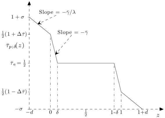
Figure 3: The piecewise linear background profile $\bar{\tau}_{\delta}(z)$, with $\bar{\tau}^{\prime}=-\bar{\gamma}/\lambda$ in the plates, $\bar{\tau}^{\prime}=-\bar{\gamma}$ in the fluid boundary layer, and $\bar{\tau}^{\prime}=0$ in the bulk.

The intuition behind this definition is that in order for $\bar{\tau}(z)$ to be strongly admissible, the indefinite term $\int_{f}2\bar{\tau}^{\prime}w\theta$ in $\mathcal{Q}_{\bar{\tau},R_{\mathrm{e}}}[\mathbf{v},\theta]$ (see (4.21)) should be controlled by the other, positive terms. With this choice of background, $2\bar{\tau}^{\prime}w\theta$ vanishes in the bulk of the fluid domain, and is nonzero only near the fluid boundaries, where $w$ and $w_{z}$ are small. Furthermore, since $\bar{\tau}^{\prime}$ is piecewise constant, explicit analytical bounds are readily attainable, giving (non-optimal) rigorous bounds on the Nusselt number.

Observe that in the fluid region $0\leq z\leq 1$, $\bar{\tau}_{\delta}(z)$ is reminiscent of observed mean temperature profiles in convection, with strong gradients in a narrow thermal boundary layer of width $\sim\delta_{\text{BL}}$ near the boundaries and approximately constant temperature in the bulk. This suggests that $\delta$ might be interpreted as modelling the thickness of the thermal boundary layer (see also the discussion following (6.14) below).

Since the background $\bar{\tau}_{\delta}$ defined in (5.1) should satisfy the BCs (4.2), we must have $\bar{\tau}_{\delta}(-d)=\bar{\tau}_{a}+\bar{\gamma}\delta+\bar{\gamma}d/\lambda=\bar{\tau}_{a}+\bar{\gamma}(\delta+\sigma)=1+\sigma$ and $\bar{\tau}_{\delta}(1+d)=\bar{\tau}_{a}-\bar{\gamma}(\delta+\sigma)=-\sigma$; solving for $\bar{\gamma}$ and for $\bar{\tau}_{a}$ (for $\sigma<\infty$), we find

$$\bar{\gamma}=\frac{1+2\sigma}{2(\delta+\sigma)},\qquad\bar{\tau}_{a}=\frac{1}{2},$$ (5.2)

completing the specification of the background $\bar{\tau}_{\delta}(z)$. We can now compute

$$\Delta\bar{\tau}=\bar{\tau}_{\delta}(0)-\bar{\tau}_{\delta}(1)=2\bar{\gamma}\delta=\frac{\delta(1+2\sigma)}{\delta+\sigma}=1+2\sigma(1-\bar{\gamma})$$

(compare (B.5)); since $\delta\leq 1/2$, we remark that $1\leq\bar{\gamma}\leq 1/2\delta$ and $\Delta\bar{\tau}\leq 1$. It follows also that $\bar{\tau}_{\delta}(0)=\bar{\tau}_{a}+\bar{\gamma}\delta=\tfrac{1}{2}(1+\Delta\bar{\tau})=1+\sigma-\sigma\bar{\gamma}$ and $\bar{\tau}_{\delta}(1)=\tfrac{1}{2}(1-\Delta\bar{\tau})=-\sigma+\sigma\bar{\gamma}$, which shows that

$$\bar{\tau}_{\delta}-\sigma\bar{\tau}_{\delta}^{\prime}=1+\sigma\ \ \text{at}\ \ z=0+\,,\qquad\bar{\tau}_{\delta}+\sigma\bar{\tau}_{\delta}^{\prime}=-\sigma\ \ \text{at}\ \ z=1-\,:$$ (5.3)

at the fluid boundaries $z=0+$ and $z=1-$, the piecewise linear background in the presence of plates $\bar{\tau}_{\delta}(z)$ satisfies the mixed thermal BCs (2.17) with Biot number $\eta=\sigma$.

To evaluate the bound (4.26), (4.27) for this background profile, we compute

$$\frac{1}{A}\left\{\bar{\tau}^{\prime 2}\right\} =\lambda\int_{-d}^{0}\bar{\tau}^{\prime 2}\,dz+\int_{0}^{1}\bar{\tau}^{\prime 2}\,dz+\lambda\int_{1}^{1+d}\bar{\tau}^{\prime 2}\,dz=\lambda d\left(\frac{\bar{\gamma}}{\lambda}\right)^{2}+2\delta\bar{\gamma}^{2}+\lambda d\left(\frac{\bar{\gamma}}{\lambda}\right)^{2}$$

$$=2\bar{\gamma}^{2}(\delta+\sigma)=\bar{\gamma}(1+2\sigma).$$ (5.4)

Substituting, the upper bound (4.26) on $\beta$ and lower bound (4.27) on $\Delta T$ in the presence of conductive plates using a piecewise linear (pwl) background then take the simple form

$$\beta\leq\bar{\mathcal{B}}_{\mathrm{pwl},\sigma}(\delta,b)\equiv\bar{\mathcal{B}}_{\sigma}[\bar{\tau}_{\delta};b] =1+b\frac{1-2\delta}{2(\delta+\sigma)}=1+b(\bar{\gamma}-1),$$ (5.5)

$$\Delta T\geq\bar{\mathcal{D}}_{\mathrm{pwl},\sigma}(\delta,b)\equiv\bar{\mathcal{D}}_{\sigma}[\bar{\tau}_{\delta};b] =1-b\frac{\sigma(1-2\delta)}{\delta+\sigma}=1+b(\Delta\bar{\tau}-1);$$ (5.6)

and the corresponding upper bound on the Nusselt number is $\mathit{Nu}=\beta/\Delta T\leq\bar{\mathcal{N}}_{\mathrm{pwl},\sigma}(\delta,b)=\bar{\mathcal{B}}_{\mathrm{pwl},\sigma}(\delta,b)/\bar{\mathcal{D}}_{\mathrm{pwl},\sigma}(\delta,b)$. Since $b>0$, these bounds satisfy $\bar{\mathcal{B}}_{\mathrm{pwl},\sigma}(\delta,b)\geq 1$, $\bar{\mathcal{D}}_{\mathrm{pwl},\sigma}(\delta,b)\leq 1$, and hence $\bar{\mathcal{N}}_{\mathrm{pwl},\sigma}(\delta,b)\geq 1$, as one might expect. Observe that the bounds $\bar{\mathcal{B}}_{\mathrm{pwl},\sigma}(\delta,b)$ and $\bar{\mathcal{D}}_{\mathrm{pwl},\sigma}(\delta,b)$ do not depend explicitly on the control parameter $R$, but rather indirectly through the admissibility condition on $\delta$. It remains, in § 5.3, to find conditions on $\delta$ for which $\bar{\tau}_{\delta}(z)$ is (strongly) admissible.

5.2 Correspondence between bounding problems with and without plates

The preceding §§ 3.2–5.1 concern the formulation of a bounding principle, and the derivation of explicit formulae for the bounds on $\beta$ and $\Delta T$ in the case of piecewise linear background fields $\bar{\tau}_{\delta}$, for Rayleigh-Bénard convection in a fluid bounded by conducting plates with dimensionless thickness $d$ and conductivity $\lambda$. In Appendix B, convection with Robin thermal BCs of fixed Biot number $\eta$ at the fluid boundaries is treated analogously.

The details of the calculations for these two cases differ at various points, when it is necessary to consider the contributions of the plates on the one hand, or of boundary terms on the other. At the level of the strong admissibility criterion for background fields and of formulae for the bounds for piecewise linear backgrounds with a given $\delta$, however, the problems with and without plates map onto one another when $\eta=\sigma=d/\lambda$:

As pointed out in § 4.3, the strong admissibility criterion on a background $\bar{\tau}(z)$ for the full plate-fluid-plate system, $\mathcal{Q}_{\bar{\tau},R_{\mathrm{e}}}[\mathbf{v},\theta]\geq 0$ for $\mathcal{Q}_{\bar{\tau},R_{\mathrm{e}}}$ defined in (4.21), depends only on the restriction of $\bar{\tau}$ onto the fluid domain $z\in[0,1]$. Consequently, for a given $R_{\mathrm{e}}$ it coincides with the strong admissibility criterion of Appendix B.2 on $\tau(z)$ for convection with thermal BCs applied to the fluid boundaries, $\mathcal{Q}_{\tau,R_{\mathrm{e}}}[\mathbf{v},\theta]\geq 0$ for the quadratic form $\mathcal{Q}_{\tau,R_{\mathrm{e}}}$ from (B.12). This is because in both criteria we optimize over the same classes of fields $\mathbf{v}$ and $\theta$, as no BCs on $\theta$ are assumed.

Of course the background fields with and without plates, $\bar{\tau}(z)$ and $\tau(z)$, should satisfy their appropriate thermal BCs, (4.2)–(4.3) or (2.17), respectively. However, for plates with a given $d$ and $\lambda$, (5.3) shows that the piecewise linear background $\bar{\tau}_{\delta}$, defined in (5.1) and satisfying (4.2)–(4.3), automatically also satisfies mixed BCs with Biot number $\eta=\sigma=d/\lambda$. Thus for a given $\delta$, over the fluid domain $0\leq z\leq 1$, $\bar{\tau}_{\delta}(z)$ coincides with $\tau_{\delta}(z)$ defined in (B.23) (so that also $\bar{\gamma}=\gamma$, $\Delta\bar{\tau}=\Delta\tau$). That is, for a given $R_{\mathrm{e}}$ a piecewise linear background $\bar{\tau}_{\delta}$ is strongly admissible in the sense of § 4.3 (this is a condition on $\delta$) if and only if its restriction $\tau_{\delta}=\bar{\tau}_{\delta}|_{[0,1]}$ is strongly admissible in the sense of Appendix B.2.

Furthermore, comparing (5.5)–(5.6) with (B.26)–(B.27), the corresponding bounds due to strongly admissible piecewise linear backgrounds at a given $\delta$ agree: $\bar{\mathcal{B}}_{\mathrm{pwl},\sigma}(\delta,b)=\mathcal{B}_{\mathrm{pwl},\eta}(\delta,b)$ and $\bar{\mathcal{D}}_{\mathrm{pwl},\sigma}(\delta,b)=\mathcal{D}_{\mathrm{pwl},\eta}(\delta,b)$ for $\sigma=\eta$.

In this analysis we have thus systematically mapped the conservative bounding problem with imperfectly conducting plates onto that with mixed BCs with the fixed Biot number $\eta=d/\lambda$. In the following sections, we discuss bounds for convection for these two problems simultaneously, assuming $\eta=\sigma=d/\lambda$. The results are presented mainly in the notation of Appendix B, using $\eta$, $\tau_{\delta}$, $\gamma$ and $\Delta\tau$, recalling that for piecewise linear backgrounds with the same $\delta$, we also have $\bar{\gamma}=\gamma$, $\Delta\bar{\tau}=\Delta\tau$, and $\bar{\tau}_{\delta}|_{[0,1]}=\tau_{\delta}$.

5.3 Cauchy-Schwarz estimates on the quadratic form

Recall the strong admissibility criterion for the background field $\tau_{\delta}(z)$: $\mathcal{Q}_{\tau_{\delta},R_{\mathrm{e}}}[\mathbf{v},\theta]\geq 0$, or in Fourier space (by (4.24)–(4.25)) $\mathcal{Q}_{\mathbf{k}}=\mathcal{Q}_{\mathbf{k};\tau_{\delta},R_{\mathrm{e}}}[\hat{w}_{\mathbf{k}},\hat{\theta}_{\mathbf{k}}]\geq 0$ for all $\mathbf{k}$ and for all sufficiently smooth (complex-valued) functions $\hat{w}_{\mathbf{k}}(z)$, $\hat{\theta}_{\mathbf{k}}(z)$, where $\hat{w}_{\mathbf{k}}$ satisfies $\hat{w}_{\mathbf{k}}=\mathrm{D}\hat{w}_{\mathbf{k}}=0$ at $z=0,1$ while no BCs are assumed for $\hat{\theta}_{\mathbf{k}}$. (However, thermal BCs enter the strong admissibility condition through the BCs for $\tau_{\delta}$, which fix the value of $\gamma$ for given $\delta$ and $\eta$.). For piecewise linear background fields $\tau_{\delta}(z)$ of the form (B.23) (or $\bar{\tau}_{\delta}(z)$ as in (5.1)), this criterion reduces to a requirement that $\delta$ is sufficiently small, for given $R_{\mathrm{e}}=bR/(b-1)$.

Elementary Cauchy-Schwarz and Young inequalities applied to the Fourier space quadratic form $\mathcal{Q}_{\mathbf{k}}$ allow us to derive explicit sufficient conditions on $\delta$ so that $\mathcal{Q}_{\mathbf{k}}\geq 0$ for all $\mathbf{k}$, and hence to estimate upper bounds on $\mathit{Nu}$. To do so, we need to control the only indefinite term in $\mathcal{Q}_{\mathbf{k}}$, $\int_{0}^{1}2\tau_{\delta}^{\prime}\text{Re}[\hat{w}_{\mathbf{k}}{\hat{\theta}_{\mathbf{k}}}^{*}]$, by the other terms. For completeness we review the necessary estimates from Otero et al. (2002): Since $\hat{w}_{\mathbf{k}}$ and $\mathrm{D}\hat{w}_{\mathbf{k}}$ (and hence also $\hat{w}_{\mathbf{k}}\,{\hat{\theta}_{\mathbf{k}}}^{*}$) vanish at both boundaries, we have

$$|\hat{w}_{\mathbf{k}}(z)\,{\hat{\theta}_{\mathbf{k}}}^{*}(z)|=\left|\int_{0}^{z}\mathrm{D}\left(\hat{w}_{\mathbf{k}}{\hat{\theta}_{\mathbf{k}}}^{*}\right)\,d\zeta\right|\leq\int_{0}^{z}|\hat{w}_{\mathbf{k}}\mathrm{D}{\hat{\theta}_{\mathbf{k}}}^{*}|\,d\zeta+\int_{0}^{z}|{\hat{\theta}_{\mathbf{k}}}^{*}\mathrm{D}\hat{w}_{\mathbf{k}}|\,d\zeta,$$ (5.7)

where for $0\leq z\leq\tfrac{1}{2}$, by the Fundamental Theorem of Calculus and the Cauchy-Schwarz inequality we find that

$$\left|\hat{w}_{\mathbf{k}}(z)\right|=\left|\int_{0}^{z}\mathrm{D}\hat{w}_{\mathbf{k}}\,d\zeta\right| \leq\sqrt{z}\left(\int_{0}^{z}\left|\mathrm{D}\hat{w}_{\mathbf{k}}(\zeta)\right|^{2}\,d\zeta\right)^{1/2}\leq\sqrt{z}\|\mathrm{D}\hat{w}_{\mathbf{k}}\|_{[0,\tfrac{1}{2}]},$$ (5.8)

$$\left|\mathrm{D}\hat{w}_{\mathbf{k}}(z)\right|=\left|\int_{0}^{z}\mathrm{D}^{2}\hat{w}_{\mathbf{k}}\,d\zeta\right| \leq\sqrt{z}\left(\int_{0}^{z}\left|\mathrm{D}^{2}\hat{w}_{\mathbf{k}}(\zeta)\right|^{2}\,d\zeta\right)^{1/2}\leq\sqrt{z}\|\mathrm{D}^{2}\hat{w}_{\mathbf{k}}\|_{[0,\tfrac{1}{2}]}.$$ (5.9)

Substituting these estimates into (5.7) and again applying the Cauchy-Schwarz inequality, for $0\leq z\leq\tfrac{1}{2}$ we obtain

$$|\hat{w}_{\mathbf{k}}(z)\,{\hat{\theta}_{\mathbf{k}}}^{*}(z)| \leq\left(\int_{0}^{z}\zeta\,d\zeta\right)^{1/2}\left[\|\mathrm{D}\hat{w}_{\mathbf{k}}\|_{[0,\tfrac{1}{2}]}\left(\int_{0}^{z}|\mathrm{D}\hat{\theta}_{\mathbf{k}}|^{2}\,d\zeta\right)^{1/2}\right.$$

$$\qquad\qquad\qquad\quad\ \left.+\|\mathrm{D}^{2}\hat{w}_{\mathbf{k}}\|_{[0,\tfrac{1}{2}]}\left(\int_{0}^{z}|\hat{\theta}_{\mathbf{k}}|^{2}\,d\zeta\right)^{1/2}\right]$$

$$\leq\frac{z}{2\sqrt{2}}\left[a_{1}\|\mathrm{D}\hat{w}_{\mathbf{k}}\|_{[0,\tfrac{1}{2}]}^{2}+\frac{1}{a_{1}}\|\mathrm{D}\hat{\theta}_{\mathbf{k}}\|_{[0,\tfrac{1}{2}]}^{2}+\frac{a_{2}}{k^{2}}\|\mathrm{D}^{2}\hat{w}_{\mathbf{k}}\|_{[0,\tfrac{1}{2}]}^{2}+\frac{k^{2}}{a_{2}}\|\hat{\theta}_{\mathbf{k}}\|_{[0,\tfrac{1}{2}]}^{2}\right],$$ (5.10)

where we have also applied Young’s inequality $pq\leq\tfrac{1}{2}(a_{j}p^{2}+q^{2}/a_{j})$ for any $a_{j}>0$. Proceeding similarly, we obtain an analogous estimate for $\tfrac{1}{2}\leq z\leq 1$.

For the piecewise linear background $\tau_{\delta}(z)$, for which $\tau_{\delta}^{\prime}=-\gamma<0$ for $0\leq z\leq\delta$ and $1-\delta\leq z\leq 1$, and $\tau_{\delta}^{\prime}=0$ otherwise, applying these estimates we have

$$\left|\int_{0}^{1}\tau_{\delta}^{\prime}\,\hat{w}_{\mathbf{k}}{\hat{\theta}_{\mathbf{k}}}^{*}\,dz\right| \leq\gamma\left(\int_{0}^{\delta}|\hat{w}_{\mathbf{k}}{\hat{\theta}_{\mathbf{k}}}^{*}|\,dz+\int_{1-\delta}^{1}|\hat{w}_{\mathbf{k}}{\hat{\theta}_{\mathbf{k}}}^{*}|\,dz\right)$$

$$\leq\frac{\gamma\delta^{2}}{4\sqrt{2}}\left[a_{1}\|\mathrm{D}\hat{w}_{\mathbf{k}}\|_{[0,1]}^{2}+\frac{1}{a_{1}}\|\mathrm{D}\hat{\theta}_{\mathbf{k}}\|_{[0,1]}^{2}+\frac{a_{2}}{k^{2}}\|\mathrm{D}^{2}\hat{w}_{\mathbf{k}}\|_{[0,1]}^{2}+\frac{k^{2}}{a_{2}}\|\hat{\theta}_{\mathbf{k}}\|_{[0,1]}^{2}\right],$$

and thus

$$\int_{0}^{1}2\tau_{\delta}^{\prime}\text{Re}[\hat{w}_{\mathbf{k}}{\hat{\theta}_{\mathbf{k}}}^{*}]\,dz =\int_{0}^{1}\tau_{\delta}^{\prime}\left(\hat{w}_{\mathbf{k}}{\hat{\theta}_{\mathbf{k}}}^{*}+{\hat{w}_{\mathbf{k}}}^{*}\hat{\theta}_{\mathbf{k}}\right)\,dz$$

$$\geq-\frac{\gamma\delta^{2}}{2\sqrt{2}}\left[a_{1}\|\mathrm{D}\hat{w}_{\mathbf{k}}\|^{2}+\frac{1}{a_{1}}\|\mathrm{D}\hat{\theta}_{\mathbf{k}}\|^{2}+\frac{a_{2}}{k^{2}}\|\mathrm{D}^{2}\hat{w}_{\mathbf{k}}\|^{2}+\frac{k^{2}}{a_{2}}\|\hat{\theta}_{\mathbf{k}}\|^{2}\right],$$ (5.11)

where norms are taken over the entire interval $[0,1]$ unless otherwise indicated. Substituting this estimate on the indefinite term into $\mathcal{Q}_{\mathbf{k}}$ given by (4.25), we find

$$\mathcal{Q}_{\mathbf{k}} \geq\left(\frac{2}{R_{\mathrm{e}}}-\frac{\gamma\delta^{2}\,a_{1}}{2\sqrt{2}}\right)\|\mathrm{D}\hat{w}_{\mathbf{k}}\|^{2}+\left(\frac{1}{R_{\mathrm{e}}}-\frac{\gamma\delta^{2}\,a_{2}}{2\sqrt{2}}\right)\frac{1}{k^{2}}\|\mathrm{D}^{2}\hat{w}_{\mathbf{k}}\|^{2}+\frac{1}{R_{\mathrm{e}}}k^{2}\|\hat{w}_{\mathbf{k}}\|^{2}$$

$$\qquad+\left(1-\frac{\gamma\delta^{2}}{2\sqrt{2}\,a_{2}}\right)k^{2}\|\hat{\theta}_{\mathbf{k}}\|^{2}+\left(1-\frac{\gamma\delta^{2}}{2\sqrt{2}\,a_{1}}\right)\|\mathrm{D}\hat{\theta}_{\mathbf{k}}\|^{2}.$$

In the absence of any additional a priori information, for instance on the decay rate of the Fourier coefficients (compare Constantin & Doering (1996); Kerswell (2001)), our remaining estimates are necessarily $k$-independent; we ensure the positivity of $\mathcal{Q}_{\mathbf{k}}$ by requiring all coefficients to be nonnegative. We choose $a_{1}=a_{2}=\gamma\delta^{2}/2\sqrt{2}$; then, dropping manifestly nonnegative terms,

$$\mathcal{Q}_{\mathbf{k}}\geq\left(\frac{2}{R_{\mathrm{e}}}-\frac{\gamma^{2}\delta^{4}}{8}\right)\|\mathrm{D}\hat{w}_{\mathbf{k}}\|^{2}+\left(\frac{1}{R_{\mathrm{e}}}-\frac{\gamma^{2}\delta^{4}}{8}\right)\frac{1}{k^{2}}\|\mathrm{D}^{2}\hat{w}_{\mathbf{k}}\|^{2}.$$ (5.12)

We can thus guarantee that $\mathcal{Q}_{\mathbf{k}}\geq 0$ independent of $\mathbf{k}$ (and hence that $\tau_{\delta}$ is strongly admissible) if we choose $\gamma^{2}\delta^{4}/8\leq 1/R_{\mathrm{e}}$. For given thermal BCs, $\gamma=\gamma(\delta)$ is specified as a function of $\delta$; so this is a constraint on $\delta$ to have $\mathcal{Q}_{\mathbf{k}}\geq 0$, that is, for $\tau_{\delta}(z)$ to be an admissible background. Defining $\delta_{c}$ by

$$\gamma(\delta_{c})^{2}\delta_{c}^{4}=\frac{(1+2\eta)^{2}}{4(\delta_{c}+\eta)^{2}}\delta_{c}^{4}=\frac{8}{R_{\mathrm{e}}}=8\frac{b-1}{bR},$$ (5.13)

we obtain the best bound in this approach by choosing $\delta=\delta_{c}$; the piecewise linear profile $\tau_{\delta}$ (or $\bar{\tau}_{\delta}$) is strongly admissible for any $\delta\leq\delta_{c}$.

6 Explicit asymptotic bounds for convection with thin, highly conductive plates or mixed thermal boundary conditions

Using piecewise linear background profiles and the estimates in § 5.3, we may now derive explicit analytical bounds on the growth of the Nusselt number $\mathit{Nu}$ with the control parameter $R$, and hence with the Rayleigh number $\mathit{Ra}$.

The results are described below mainly in terms of the mathematical idealization of mixed (Robin) thermal BCs with Biot number $\eta$, showing that one may interpolate between the fixed temperature (Dirichlet) and fixed flux (Neumann) limits in a unified formulation. However, as discussed in § 5.2, all results apply also to the more physical problem of a convection in a fluid bounded by imperfectly conducting plates of finite, nonzero (scaled) thickness $d$ and conductivity $\lambda$, when $\eta=\sigma\in(0,\infty)$. We shall remark on possible interpretations of our results for convection with plates when appropriate.

In this Section we summarize the main asymptotic bounds; more details, including improved values of the prefactors obtained by numerical solution of the optimization problem for piecewise linear background profiles, are given elsewhere (Wittenberg & Gao (2010)). The asymptotic analytical and the numerical bounds obtained using piecewise linear background functions differ only in their prefactors; the scaling with respect to $R$ and $\eta$ (or $\sigma$) is the same in each case.

We begin by reviewing the results for Dirichlet ($\eta=0$) and Neumann ($\eta=\infty$) BCs, since in the general case, depending on the relative sizes of $\delta$ and $\eta$, the scaling behaviour agrees with one or the other of these extremes. In fact we shall see that for any $\eta>0$, the $R\to\infty$ asymptotic scaling behaviour is as in the fixed flux case.

6.1 Fixed temperature boundary conditions

In the case of Dirichlet BCs ($\eta=0$ or $\sigma=0$), we have $\Delta T=\Delta\tau=1$, $R=\mathit{Ra}$, and (B.25) implies $\gamma=1/2\delta$. Thus the sufficient condition (5.13) on $\delta$ simplifies to $\delta\leq\delta_{c}$ where

$$\delta_{c}^{2}=\frac{32}{R_{\mathrm{e}}}=32\frac{b-1}{bR}.$$ (6.1)

One can show that the optimal choice of $b$ in this formulation is $b_{0}=3/2$ (see Wittenberg & Gao (2010)), for which $R_{\mathrm{e}}=3R$, and hence $\delta\leq\delta_{c}=4\sqrt{2/3}\,R^{-1/2}$ is sufficient to obtain a rigorous bound. Since for this $b=b_{0}$, (B.26) becomes

$$\mathit{Nu}=\beta\leq\mathcal{B}_{\mathrm{pwl},0}(\delta,b_{0})=1-b_{0}+\frac{b_{0}}{2\delta}=-\frac{1}{2}+\frac{3}{4\delta},$$ (6.2)

for any $\delta\leq\delta_{c}$, the best rigorous analytical bound on the Nusselt number using this approach, valid for all $R$ sufficiently large that $\delta_{c}\leq 1/2$, is

$$\mathit{Nu}\leq\mathcal{B}_{\mathrm{pwl},0}(\delta_{c},b_{0})=-\frac{1}{2}+\frac{3}{4\delta_{c}}=-\frac{1}{2}+\frac{3}{16}\sqrt{\frac{3}{2}}R^{1/2}=-\frac{1}{2}+\frac{3\sqrt{6}}{32}\mathit{Ra}^{1/2},$$ (6.3)

where we used the fact that for fixed temperature BCs, the control parameter $R$ is the usual Rayleigh number $\mathit{Ra}$.

6.2 Fixed flux boundary conditions

In the opposite extreme, for Neumann BCs ($\eta=\infty$), we have $\beta=\gamma=1$, so $\Delta\tau=2\delta$ from (B.24), and we bound $\Delta T$ from below using (B.27). Since $b>1$, in order for the lower bound $\mathcal{D}_{\mathrm{pwl},\infty}(\delta,b)=1-b+2\delta\,b$ on $\Delta T$ to remain positive as $R\to\infty$ ($\delta\to 0$), we need $b-1={\mathcal{O}}(\delta)$. Thus following Otero et al. (2002) we choose $b=1+c\,\delta$ and let $c$ take its optimal value $c_{\infty}=1/2$, so that the bound on $\Delta T$ becomes

$$\mathit{Nu}^{-1}=\Delta T\geq\mathcal{D}_{\mathrm{pwl},\infty}(\delta,1+c_{\infty}\delta)=1+(1+\delta/2)(2\delta-1)=\frac{3}{2}\delta+\delta^{2}\sim\frac{3}{2}\delta.$$ (6.4)

The condition on $\delta$ is as usual $\delta\leq\delta_{c}$, where with $\gamma=1$ and $b=1+\delta/2$, the equation (5.13) satisfied by $\delta_{c}$ takes the form

$$\delta^{4}=\frac{8}{R_{\mathrm{e}}}=4\frac{\delta}{1+\delta/2}R^{-1}\sim 4\frac{\delta}{R}$$ (6.5)

for large $R$, for which $\delta\to 0$; and hence $\delta_{c}\sim 4^{1/3}R^{-1/3}$. Thus we have (using (3.3))

$$\mathit{Nu}^{-1}=\Delta T \geq\mathcal{D}_{\mathrm{pwl},\infty}(\delta_{c},1+\delta_{c}/2)\sim\frac{3}{2}\delta_{c}\sim\frac{3}{2^{1/3}}R^{-1/3},$$

$$\mathit{Ra}=R\Delta T \geq R\,\mathcal{D}_{\mathrm{pwl},\infty}(\delta_{c},1+\delta_{c}/2)\sim\frac{3}{2^{1/3}}R^{2/3},$$

and so

$$\mathit{Nu}\lesssim\frac{2^{1/3}}{3}R^{1/3}\lesssim\sqrt{\frac{2}{27}}\mathit{Ra}^{1/2},$$ (6.6)

as in Otero et al. (2002). Note the scaling $\mathit{Nu}\leq C_{1}R^{1/3}$ in terms of the control parameter $R$, which translates to the usual scaling $\mathit{Nu}\leq C_{2}\mathit{Ra}^{1/2}$.

6.3 Mixed thermal boundary conditions

For general mixed (Robin) thermal BCs with fixed Biot number $\eta$ (or equivalently, for plates with nonzero, finite $\sigma=d/\lambda$), we need to estimate both $\Delta T$ and $\beta$, using (B.26) and (B.27), where $\gamma$ and $\Delta\tau$ are given in terms of $\eta$ and $\delta$ by (B.25). The sufficient condition $\delta\leq\delta_{c}$ for $\tau_{\delta}$ to be (strongly) admissible, derived via the Cauchy-Schwarz estimates of § 5.3, is that $\delta_{c}$ satisfies (5.13), which (substituting for $\gamma$ from (B.25)) here takes the form

$$\gamma^{2}\delta^{4}=\frac{(1+2\eta)^{2}}{4(\delta+\eta)^{2}}\delta^{4}=\frac{8}{R_{\mathrm{e}}}=8\frac{b-1}{b}R^{-1}.$$ (6.7)

We shall see that in this general case with $0<\eta<\infty$, the scaling of the bounds depends on the relative sizes of $\delta$ and $\eta$, behaving either as in the fixed temperature limit (for $\delta\geq\eta$) or the fixed flux limit (for $\delta\leq\eta$); but that for any $\eta>0$, the asymptotic scaling properties as $R\to\infty$ are as for fixed flux boundary conditions:

The fixed temperature problem $\eta=0$ as a singular limit:

Recall that for Dirichlet thermal boundary conditions $\eta=0$, we have $\Delta T=\Delta\tau=1$, so that we obtain an upper bound on $\mathit{Nu}$ for any $b>0$ (there is no concern that the lower bound $\mathcal{D}_{\mathrm{pwl},0}$ on $\Delta T$ may become negative), and we can choose $b-1={\mathcal{O}}(1)$ for all $\delta$. In this case $\eta=0$, though, $\gamma=1/2\delta$ is not bounded above as $R\to\infty$ ($\delta\to 0$), and hence neither is $\beta$; the growth in the (upper bound for the) Nusselt number $\mathit{Nu}=\beta$ in the fixed temperature case with increasing control parameter $R=\mathit{Ra}$ is due to that of the (non-dimensional) boundary heat flux.

The situation is quite different for any nonzero Biot number $\eta$: since $0<\delta\leq 1/2$, we have $0\leq(1-2\delta)/2(\delta+\eta)=\gamma-1<1/2\eta$, so that for each $\eta>0$, now $\gamma$ is bounded above as $\delta\to 0$. From (B.26) (and choosing $b\leq 2$) it follows that for all $\eta>0$, we have the rigorous (though presumably weak) upper bound on the boundary heat flux

$$\beta\leq 1+\frac{b}{2\eta}\leq 1+\frac{1}{\eta}\ ;$$ (6.8)

that is, $\beta$ saturates at a finite value as $R\to\infty$. On the other hand, the (non-dimensional) averaged temperature drop across the fluid $\Delta T$ is not bounded below away from zero: $\Delta T\to 0$. Hence asymptotically for large $R$, the growth in the Nusselt number $\mathit{Nu}=\beta/\Delta T$ (and in the corresponding bound) is due to the decrease in $\Delta T$, rather than due to growth of $\beta$. That is, for any $\eta>0$ the (asymptotic) behaviour and scaling is as in the fixed flux case; the fixed temperature problem is a singular limit of the bounding problem. (A similar observation was made in the context of horizontal convection by Siggers et al. (2004).)

Scaling for poorly conducting boundaries:

The nature of the $\mathit{Nu}$-$R$ scaling depends on whether $\delta\geq\eta$ or $\delta\leq\eta$, and hence on the value of $\eta$. For sufficiently large Biot number (largely insulating boundary) $\eta\geq 1/2$, we always have $\delta\leq\eta$. Since for such $\eta$, $\gamma$ is approximately constant ($1\leq\gamma<1+1/2\eta\leq 2$; compare $\gamma=1$ for $\eta=\infty$), we see from (6.7) that a sufficient admissibility condition for $\tau_{\delta}$ is $\delta\leq\delta_{c}={\mathcal{O}}(R_{\mathrm{e}}^{-1/4})$, as in the fixed flux case. We choose $b=1+c\delta\leq 3/2$ for some $c\leq 1$, so $\beta\leq 1+b(\gamma-1)\leq 5/2$, and there is no transition in scaling regimes; as in the fixed flux case, for all sufficiently large $\eta$ the growth in $\mathit{Nu}$ with increasing $R$ is due to the decrease in $\Delta T$. This conclusion equivalently holds for thick and/or poorly conducting plates for which $\sigma=d/\lambda\gtrsim{\mathcal{O}}(1)$.

Scaling regimes for highly conductive plates:

For relatively small Biot number (largely conducting boundary) $\eta<1/2$, on the other hand, it is possible to have $\delta\geq\eta$ for low enough thermal driving, thereby allowing for different scaling behaviours. In particular, we consider the case of small Biot number ($\eta\ll 1$, near the fixed temperature limit). This is relevant (by the correspondence $\sigma=\eta$) to convection in a fluid bounded by conductive plates in the physically relevant limit of $0<\sigma=d/\lambda\ll 1$; some implications for that situation are discussed in § 6.4.

As the control parameter $R$ increases, one observes a transition between two distinct scaling regimes:

Low Rayleigh numbers: the “fixed temperature” limit:
For sufficiently small $R$, we have $\delta\gg\eta$; in this limit, we find $\gamma\approx 1/2\delta$ and $\Delta\tau\approx 1$, and the sufficiency condition (6.7) is $\delta\leq\delta_{c}={\mathcal{O}}(R_{\mathrm{e}}^{-1/2})$. Since $\Delta\tau$ is bounded below away from zero, so is the lower bound $\mathcal{D}_{\mathrm{pwl},\eta}(\delta,b)=1+b(\Delta\tau-1)\geq 1-b/2$ on $\Delta T$ for any fixed $b<2$. Thus we may obtain a bound on $\mathit{Nu}$ in this regime by choosing any $b\in(1,2)$, and by comparison with the fixed temperature problem, it is sufficient to choose $b-1={\mathcal{O}}(1)$, so that the “effective control parameter” $R_{\mathrm{e}}=bR/(b-1)$ is proportional to $R$, and $\delta_{c}={\mathcal{O}}(R^{-1/2})$.

It follows that the bounds on $\beta$ and $\Delta T$ scale as $\beta\leq\mathcal{B}_{\mathrm{pwl},\eta}(\delta,b)=1+b(\gamma-1)={\mathcal{O}}(\delta^{-1})={\mathcal{O}}(R^{1/2})$ and $\Delta T\geq\mathcal{D}_{\mathrm{pwl},\eta}={\mathcal{O}}(1)$; hence the growth in the Nusselt number is due to the growth in the dimensionless averaged boundary heat flux, $\mathit{Nu}=\beta/\Delta T\leq\mathcal{N}_{\mathrm{pwl},\eta}={\mathcal{O}}(\delta^{-1})={\mathcal{O}}(R^{1/2})$. Furthermore, we have $\mathit{Ra}=R\Delta T\approx R$, so that the control parameter approximately coincides with the usual Rayleigh number in this case, and we have $\delta={\mathcal{O}}(\mathit{Ra}^{-1/2})$, and $\mathit{Nu}\leq C_{1}\mathit{Ra}^{1/2}$ for some $\eta$-independent constant $C_{1}$. Hence when $\eta\ll 1$, for sufficiently small $R$, everything scales as in the fixed temperature case.

Transition:
As the control parameter $R$ increases, $\delta$ shrinks, eventually decreasing below the Biot number $\eta$; the system then enters another scaling regime, in which the above estimates no longer apply. The transition at $\delta\approx\eta$ occurs (based on the low-$R$ “fixed temperature” scaling, which gives $\delta={\mathcal{O}}(R^{-1/2})={\mathcal{O}}(\mathit{Ra}^{-1/2})$ in our formalism) for

$$R\approx R_{\mathrm{t}}={\mathcal{O}}(\eta^{-2}),$$ (6.9)

that is, $\mathit{Ra}_{\mathrm{t}}={\mathcal{O}}(\eta^{-2})$.

High Rayleigh numbers: “fixed flux” scaling:
Once the “boundary layer thickness” $\delta$ has decreased below $\eta>0$ for increasing $R\gtrsim R_{\mathrm{t}}$, we enter another regime (which does not exist in the fixed temperature case $\eta=0$), with changes in the scaling behaviour of the bounds, and especially in the relative contributions of $\beta$ and $\Delta T$ to the Nusselt number.

In this regime, as $R\to\infty$ (that is, $\mathit{Ra}\to\infty$) for fixed $\eta$ the growth in $\gamma$ saturates, while $\Delta\tau={\mathcal{O}}(\delta)$ decreases. Asymptotically for $\delta\ll\eta\leq 1/2$, we have $\gamma\sim(1+2\eta)/2\eta=\gamma_{\text{max}}(\eta)$, while $\Delta\tau\sim\delta(1+2\eta)/\eta\ll 1$, and for each fixed $\eta>0$ the behaviour is now as if we had Neumann thermal BCs.

More generally, for $0<\eta\leq 1/2$ and decreasing $\delta\leq\eta$, we have $\gamma={\mathcal{O}}(\eta^{-1})$ and $\Delta\tau={\mathcal{O}}(\delta/\eta)$. Consequently, in order for the lower bound $\mathcal{D}_{\mathrm{pwl},\eta}=1-b+b\Delta\tau$ on $\Delta T$ from (B.27) to remain positive as $\delta\to 0$, the so far arbitrary parameter $b>1$ must be chosen as $b=1+{\mathcal{O}}(\delta/\eta)$. We then find that $\beta\leq\mathcal{B}_{\mathrm{pwl},\eta}=1+b(\gamma-1)={\mathcal{O}}(\eta^{-1})$ saturates, while $\Delta T\geq{\mathcal{O}}(\delta/\eta)$; hence the growth in $\mathit{Nu}$ is now due to the decay in $\Delta T$. In this regime the scaling behaviours are $\mathit{Ra}\geq{\mathcal{O}}(\delta R/\eta)$, $R_{\mathrm{e}}={\mathcal{O}}(\eta R/\delta)$ and

$$\delta={\mathcal{O}}\left(\eta^{1/2}R_{\mathrm{e}}^{-1/4}\right)={\mathcal{O}}\left(\eta^{1/3}R^{-1/3}\right)={\mathcal{O}}\left(\mathit{Ra}^{-1/2}\right);$$ (6.10)

more precise asymptotic statements are given below, while implications for convection with plates are in § 6.4.

Asymptotic scaling of bounds for $0<\eta<\infty$:

Having outlined the behaviour in the different regimes, we now derive the scaling of the bound on $\mathit{Nu}$ in the limit of large driving, $R\to\infty$, so that $\delta\ll 1$ and $\delta\ll\eta$; see Wittenberg & Gao (2010) for a comparison with the optimal solution for piecewise linear backgrounds $\tau_{\delta}(z)$. (As usual all these results carry over directly to convection with plates for $\sigma=\eta$.)

In the light of the previous discussion, to ensure a positive lower bound on $\Delta T$ for $\delta\ll\eta$ we must take $b=1+c\,\delta$, where the optimal value of $c$ turns out to be

$$c_{\eta}=\frac{1+2\eta}{4\eta}.$$ (6.11)

Using this optimal choice of $b$, the lower bound (B.27) on $\Delta T$ becomes

$$\Delta T\geq\mathcal{D}_{\mathrm{pwl},\eta}(\delta,1+c_{\eta}\delta) =-c_{\eta}\delta+(1+c_{\eta}\delta)\frac{\delta(1+2\eta)}{\delta+\eta}$$

$$=\frac{\delta(1+2\eta)}{\delta+\eta}\frac{3+2\delta}{4}\sim\frac{3}{4}\frac{\delta(1+2\eta)}{\eta},$$ (6.12)

while similarly, the upper bound (B.26) is

$$\beta\leq\mathcal{B}_{\mathrm{pwl},\eta}(\delta,1+c_{\eta}\delta) =-c_{\eta}\delta+(1+c_{\eta}\delta)\frac{1+2\eta}{2(\delta+\eta)}$$

$$=\frac{1+2\eta}{2(\delta+\eta)}\left[1+\frac{\delta}{4\eta}(1-2\delta)\right]\sim\frac{1+2\eta}{2\eta},$$ (6.13)

so that an upper bound on the Nusselt number for admissible $\delta\ll\eta$ is

$$\mathit{Nu}=\frac{\beta}{\Delta T}\leq\mathcal{N}_{\mathrm{pwl},\eta}(\delta,1+c_{\eta}\delta)=\frac{1}{2\delta}\frac{4+\delta(1-2\delta)/\eta}{3+2\delta}\sim\frac{2}{3\delta};$$ (6.14)

compare (6.2) and (6.4).

We remark that the width $\delta_{\text{BL}}$ of the thermal boundary layer is often related to the Nusselt number via $\delta_{\text{BL}}=(2\mathit{Nu})^{-1}$ (Niemela & Sreenivasan (2006b)); our high-$R$ result for the piecewise linear background, $\delta\sim(3\mathit{Nu}/2)^{-1}$ for $\eta>0$ (or $\delta\sim(4\mathit{Nu}/3)^{-1}$ for $\eta=0$), may be interpreted as a systematic statement of such a boundary layer model.

Returning to the computation of asymptotic bounds, we note from (6.11) that for $\eta\geq 1/2$, $c_{\eta}=1/2+1/4\eta\leq 1$, while for $\eta\leq 1/2$, $c_{\eta}\delta=(1+2\eta)\delta/4\eta\leq\delta/2\eta$, so that whenever $\delta\ll\min(\eta,1)$ we have $c_{\eta}\delta\ll 1$; consequently $b=1+c_{\eta}\delta\sim 1$ and $R_{\mathrm{e}}=b\,R/(b-1)\sim R/c_{\eta}\delta$. In this case the condition (6.7) is thus

$$\delta^{4}=32\frac{(\delta+\eta)^{2}}{(1+2\eta)^{2}}R_{\mathrm{e}}^{-1}\sim 32\frac{\eta^{2}}{(1+2\eta)^{2}}\frac{1+2\eta}{4\eta}\delta R^{-1}=8\frac{\eta}{1+2\eta}\delta R^{-1},$$ (6.15)

or $\delta_{c}\sim 2\eta^{1/3}(1+2\eta)^{-1/3}R^{-1/3}$. Substituting into the above bounds, we have

$$\mathit{Nu}\leq\mathcal{N}_{\mathrm{pwl},\eta}(\delta_{c},1+c_{\eta}\delta_{c}) \sim\frac{2}{3\,\delta_{c}}\sim\frac{1}{3}\left(\frac{1+2\eta}{\eta}\right)^{1/3}R^{1/3},$$ (6.16)

$$\mathit{Ra}=R\Delta T\geq R\mathcal{D}_{\mathrm{pwl},\eta}(\delta_{c},1+c_{\eta}\delta_{c}) \sim\frac{3}{4}\frac{1+2\eta}{\eta}\,\delta_{c}\,R\sim\frac{3}{2}\left(\frac{1+2\eta}{\eta}\right)^{2/3}R^{2/3},$$ (6.17)

so that we obtain a bound on the asymptotic scaling as $R\to\infty$ of the Nusselt number with the Rayleigh number whenever $\eta>0$:

$$\mathit{Nu}\lesssim\frac{1}{3}\left(\frac{1+2\eta}{\eta}\right)^{1/3}\sqrt{\frac{2}{3}}\left(\frac{\eta}{1+2\eta}\right)^{1/3}\mathit{Ra}^{1/2}=\sqrt{\frac{2}{27}}\mathit{Ra}^{1/2},$$ (6.18)

independent of the Biot number. Observe in particular, by comparison with (6.6), that the prefactor $\sqrt{2/27}$ is the same as for the fixed flux problem.

6.4 Heat transport in thin, highly conducting plates

It is instructive to view the above scaling results in the experimentally realistic context of conductive plates with small, but nonzero, thickness $h_{s}$ and/or large, but finite, conductivity $\lambda_{s}$, relative to the properties of the fluid. In dimensionless terms, this corresponds to fixed small, nonzero $\sigma$, since we have $0<d=h_{s}/h\ll 1$, $1\ll\lambda=\lambda_{s}/\lambda_{f}<\infty$, and thus $0<\sigma=d/\lambda\ll 1$.

Observe that in this case we have $1+2\sigma\approx 1$, so that (from (2.22) and (2.26)) $\Theta\approx\Delta^{*}=T_{l}^{*}-T_{u}^{*}$, that is, temperatures are scaled with respect to the applied temperature difference across the entire system. This allows us to interpret the control parameter

$$R=\frac{\alpha gh^{3}}{\nu_{f}\kappa_{f}}\Theta=\frac{\alpha gh^{3}}{\nu_{f}\kappa_{f}}\frac{\Delta^{*}}{1+2\sigma}\approx\frac{\alpha gh^{3}}{\nu_{f}\kappa_{f}}(T_{l}^{*}-T_{u}^{*})$$ (6.19)

as the Rayleigh number measured in terms of the imposed temperature drop across the full plate-fluid-plate system, instead of the temperature difference across the fluid only.

Letting $\delta$ be a measure of the thermal boundary layer width, for sufficiently small $R$ we have $\delta\gg\sigma$; that is, the thermal boundary layer thickness, approximated by $h\delta$, is much greater than the plate thickness scaled by the conductivity ratio, given by $h_{s}\,\lambda_{f}/\lambda_{s}$. In this limit we have $\Delta T\approx 1$, which implies that essentially the entire temperature drop across the system occurs across the fluid (and that $\mathit{Ra}\approx R$). That is, for $\sigma\ll 1$ and sufficiently small driving, the thermal behaviour of the fluid is essentially unaffected by the presence and finite conductivity of the plates, and the commonly used approximation, that the fluid boundaries are held at fixed temperature, is appropriate.

As $R$ increases, $\delta$ decreases, until eventually $\delta\approx\sigma$; this occurs for $R\approx R_{\mathrm{t}}$, where in our analysis the transition value $R_{\mathrm{t}}={\mathcal{O}}(\sigma^{-2})$ (see (6.9)). Near this transition, $\mathit{Nu}\lesssim{\mathcal{O}}(R^{1/2})={\mathcal{O}}(\sigma^{-1})={\mathcal{O}}(\lambda/d)$ (with ${\mathcal{O}}(1)$ constant prefactors), so that we can interpret the scaling transition as occurring when the effective conductivity of the fluid, measured by the Nusselt number, becomes comparable to the plate-fluid conductivity ratio, scaled by the plate-fluid thickness ratio; this is in accord with our intuition.

Once the control parameter $R$ increases beyond $R_{\mathrm{t}}$, the high-$\mathit{Ra}$ asymptotic regime is entered, in which the scaling behaviours of the bounds differ from those in the low-$\mathit{Ra}$ case. In particular, in the $R\to\infty$ limit, when $\delta\ll\sigma\ll 1$, using (5.5)–(5.6) and the $\delta$-scaling (6.10) we may estimate the bounds on $\Delta T$ and $\beta$ in this analysis to be

$$\Delta T\geq\bar{\mathcal{D}}_{\mathrm{pwl},\sigma}={\mathcal{O}}\left(\sigma^{-1}\delta\right)={\mathcal{O}}\left(\sigma^{-2/3}R^{-1/3}\right),\qquad\beta\leq\bar{\mathcal{B}}_{\mathrm{pwl},\sigma}={\mathcal{O}}\left(\sigma^{-1}\right),$$ (6.20)

and the usual Rayleigh number is related to $R$ via $\mathit{Ra}=R\Delta T\geq{\mathcal{O}}\left(\sigma^{-2/3}R^{2/3}\right)$. It is apparent that for fixed nonzero $\sigma$, for sufficiently large $\mathit{Ra}$ all the intermediate variables scale as in the fixed flux case discussed in Otero et al. (2002), as expected.

In this scaling regime, the dimensionless averaged heat flux $\beta$ through the fluid boundaries saturates, while an appreciable portion of the temperature drop across the system now occurs across the plates, whose finite thickness and conductivity become significant for $R\gtrsim R_{\mathrm{t}}$. Consequently $\mathit{Nu}$ increases no longer via growth in $\beta$, but due to the decrease in the averaged temperature drop across the fluid, as a fraction of the overall applied temperature drop, according to $\Delta T\geq{\mathcal{O}}\left(\left(R/R_{\mathrm{t}}\right)^{-1/3}\right)$. Finally, we find the high-$R$ asymptotic scaling of the bound on the Nusselt number $\mathit{Nu}=\beta/\Delta T\leq{\mathcal{O}}(\delta^{-1})$ for convection in the presence of conductive plates with $0<\sigma\ll 1$ (in this formalism, using a family of piecewise linear backgrounds and conservative Cauchy-Schwarz estimates): $\mathit{Nu}\leq\bar{\mathcal{N}}_{\mathrm{pwl},\sigma}={\mathcal{O}}\left(\sigma^{-1/2}R_{\mathrm{e}}^{1/4}\right)={\mathcal{O}}\left(\sigma^{-1/3}R^{1/3}\right)={\mathcal{O}}\left(\mathit{Ra}^{1/2}\right)$.

In summary, for Rayleigh-Bénard convection in a fluid bounded by thin, highly but not perfectly conducting plates, the main analytical results are: there exist $\sigma$-independent ${\mathcal{O}}(1)$ constants $C_{2}$ and $C_{3}$ so that as $R\to\infty$,

$$\mathit{Nu} \leq C_{2}\mathit{Ra}^{1/2},$$ (6.21)

$$\mathit{Nu} \leq C_{3}\,\sigma^{-1/3}R^{1/3}.$$ (6.22)

The scaling in (6.21) is the same as obtained elsewhere for finite Prandtl number Rayleigh-Bénard convection; in this formalism, the presence of conductive plates does not appear to alter the asymptotic scaling dependence of the Nusselt number on the usual Rayleigh number $\mathit{Ra}$.

In contrast, consider the result (6.22): while this (possibly non-optimal) bound on $\mathit{Nu}$ scales as $\mathit{Ra}^{1/2}$ in terms of the Rayleigh number measuring the averaged temperature drop across the fluid, for sufficiently large imposed temperature gradient we find that $\mathit{Nu}$ scales as $R^{1/3}$ in terms of the Rayleigh number measured across the entire system; albeit with a prefactor that grows for small $\sigma$ as $\sigma^{-1/3}$.

In an experiment with sufficiently small fixed dimensionless plate thickness $d$ and/or large conductivity ratio $\lambda$, so $\sigma=d/\lambda\ll 1$, it might seem plausible to ignore the plates and evaluate the Rayleigh number assuming that the fixed temperature difference is imposed at the boundaries of the fluid. We have shown directly from the governing PDEs that in terms of this “Rayleigh number” $R$ across the full system, for sufficiently strong heating the scaling exponent $p$ in a relationship $\mathit{Nu}\sim CR^{p}$ could be no greater than 1/3. We should emphasize though that this “1/3 scaling” in our bounds is only relevant for large $R$ (or $\mathit{Ra}$) — beyond a transition value $R_{\mathrm{t}}$ which scales, in our estimates, as $\sigma^{-2}$, and may thus for small $\sigma$ be inaccessible to experiments or direct numerical simulations — and is presumably unrelated to the exponents $p\lesssim 1/3$ seen in experiments or simulations.

7 Conclusions

For finite Prandtl number Rayleigh-Bénard convection, we have formulated the energy identities and bounding problem in the case of mixed thermal BCs with fixed Biot number $\eta$ applied at the upper and lower boundaries of the fluid, and demonstrated that the fixed temperature and fixed flux extremes may indeed be treated as special cases of a more general model, for which one can obtain rigorous analytical and asymptotic bounds on convective heat transport.

It has also come out of this formalism that, at least at the level of our conservative upper bounds with piecewise linear backgrounds, the case of convection with plates may be systematically mapped onto that with finite Biot number, via $\eta=\sigma=d/\lambda$.

While the scaling of these analytical bounds on the $\mathit{Nu}$–$\mathit{Ra}$ relationship remains well above that observed experimentally or in direct numerical simulations, some of the qualitative conclusions may be instructive. Of particular interest is that while for each fixed control parameter $R$ the bounds depend smoothly on $\eta$ for $0\leq\eta\leq\infty$, the asymptotic $R\to\infty$ behaviour of the bounding problem for any nonzero Biot number is as for the $\eta=\infty$ fixed flux problem. Indeed, we have proved that unlike in the fixed temperature case $\eta=0$, for each $\eta>0$ the averaged dimensionless boundary heat flux $\beta$ is bounded above uniformly in $R$, $\beta-1\leq\eta^{-1}$, so that the asymptotic growth in $\mathit{Nu}$ is necessarily due to decay of $\Delta T$. That is, the limits $\eta\to 0$ and $R\to\infty$ do not commute: the much-studied fixed temperature case is a singular limit of the general bounding problem. From the point of view of understanding a realistic convection situation in the limit of large $R$, it appears that the mathematical structure of the insulating-plates fixed flux problem is more relevant.

Furthermore, our analysis reveals two distinct scaling behaviours for sufficiently small nonzero $\sigma$ (or $\eta$): In the “fixed temperature scaling regime” for small Rayleigh number $\mathit{Ra}$, the growth in the (bounds on the) convective heat transport measured by $\mathit{Nu}$ is largely due to the increase in the averaged boundary heat flux $\beta$. However, for strong driving, eventually a “fixed flux scaling regime” is reached in which the effective conductivity of the fluid due to convective transport exceeds the plate conductivity, and the plates effectively act as insulators; $\beta$ saturates and further increases in $\mathit{Nu}$ are due to decreases in the averaged temperature drop $\Delta T$. The transition between these regimes occurs when the “thermal boundary layer width” $\delta$ is comparable to $\sigma$.

It would be of interest to determine whether this qualitative transition at $R\approx R_{\mathrm{t}}$ from effectively conducting to effectively insulating boundaries is in fact reflected in the physics of convective turbulence in the fluid, and thus observable in experiments with small $\sigma=d/\lambda$, or in direct numerical simulations with fixed Biot number $\eta\ll 1$. It is possible that it may not be: the recent direct numerical simulations comparing fixed temperature and fixed flux BCs, due to Johnston & Doering (2009) in two dimensions with horizontal periodicity, and to Verzicco & Sreenivasan (2008) and Stevens et al. (2010) in three-dimensional cylindrical geometry, suggest that the heat transport in large-$\mathit{Ra}$ turbulent convection appears to be insensitive to thermal boundary conditions.

In this context we observe that the prefactor in our asymptotic analytical bound $\mathit{Nu}\leq C\,\mathit{Ra}^{1/2}$ increases from $C_{0}=3\sqrt{6}/32\approx 0.230$ to $C_{\eta}=C_{\infty}=\sqrt{2/27}\approx 0.272$ for $\eta>0$; that is, within the framework of our upper bounding calculations with piecewise linear background it appears that the estimates on the heat transport increase when the boundaries are not perfectly conducting. It remains to determine whether this increase is an artifact of the choice of background $\tau(z)$ or of the background flow bounding approach in general.

Acknowledgments

I would like to thank Charlie Doering, Jian Gao, Jesse Otero and Jean-Luc Thiffeault for useful discussions concerning this work, and the anonymous referees for numerous helpful suggestions. This research was partially supported by grants from the Natural Sciences and Engineering Research Council of Canada (NSERC).

Appendix A Comments on the formulation and notation

In the following we introduce and clarify some notation used in our calculations.

Averages:

Following Otero et al. (2002), for functions $h(x,y,z)$ and $g(t)$ we define the horizontal and time averages, $\overline{h}(z)$ and $\langle g\rangle$ respectively, by

$$\overline{h}(z)=\frac{1}{A}\iint_{A}h(x,y,z)\,dxdy=\frac{1}{A}\int_{0}^{L_{y}}\int_{0}^{L_{x}}h(x,y,z)\,dxdy$$ (A.1)

and

$$\langle g\rangle=\limsup_{\tau\to\infty}\frac{1}{\tau}\int_{0}^{\tau}g(t)\,dt,$$ (A.2)

where $A=L_{x}L_{y}$ is the nondimensional area of the plates.

Global definitions in presence of plates:

The problem of Rayleigh-Bénard convection with bounding plates may be formulated using separate fields in the fluid and the lower and upper plates, with appropriate conditions at the interfaces between the different domains. However, as discussed before (2.19), for simplicity of notation it is more convenient to treat the space- and time-dependent fields as being defined across the entire plate-fluid-plate system, for $-d\leq z\leq 1+d$. (Recall that all $x$- and $y$-dependent quantities are $L_{x}$, $L_{y}$-periodic in the horizontal directions.) Thus we consider a single dimensionless temperature field $T$, which coincides with the temperature in the lower plate $T_{p,l}$ on $z\in[-d,0)$, with the fluid temperature $T_{f}$ on $z\in(0,1)$ and with the upper plate temperature $T_{p,u}$ on $z\in(1,1+d]$; it is a continuous function with discontinuous vertical derivative at $z=0$ and 1, which satisfies the conditions (2.30)–(2.31) at the fluid-plate interfaces at $z=0$ and 1, and the boundary conditions (2.32). (Equivalently, defining a piecewise constant global thermal conductivity function $\bar{\lambda}=\bar{\lambda}(z)$ which takes the values $1$ in the fluid and $\lambda$ in the plates, (2.30)–(2.31) can be interpreted as continuity conditions on both $T$ and the weighted derivative $\bar{\lambda}\,\partial T/\partial z$.) Similarly, we may extend the definition of the velocity field by $\mathbf{u}\equiv\mathbf{0}$ in the plates $-d\leq z\leq 0$ and $1\leq z\leq 1+d$; then (by the no-slip BCs $\mathbf{u}|_{z=0,1}=\mathbf{0}$) the velocity field is similarly continuous across the entire system, with discontinuous vertical derivative in the horizontal velocity components (by incompressibility, $w_{z}|_{z=0,1}=0$). Similar considerations apply to the fluctuating quantities $\mathbf{v}=\mathbf{u}$, $\theta=T-\bar{\tau}$ defined in § 4.1.

Limits and boundary terms:

For convection in the presence of plates, since the temperature field $T$ is piecewise defined, care should be taken in evaluating $T_{z}$ and related fields which are discontinuous at the interfaces $z=0$ and $1$, for instance when evaluating boundary terms upon integrating over the fluid or plates. To simplify the description, before (2.19) we introduced notation for limits, writing, for instance, $T|_{z=1+}=\lim_{z\to 1+}T=T_{p,u}|_{z=1}$, or $(\partial T/\partial z)|_{z=0+}=(\partial T_{f}/\partial z)|_{z=0}$. Similarly, we write $\left.(\cdot)\right|_{z=0+}^{1-}$ to indicate that boundary values are approached from within the fluid: specifically, for any function $f(z)$, we have

$$\left.(f)\right|_{z=0+}^{1-}\equiv f|_{z=1-}-f|_{z=0+}\equiv\lim_{z\to 1-}f-\lim_{z\to 0+}f=\int_{0}^{1}f_{z}\,dz\;;$$ (A.3)

and similarly for $\left.(f)\right|_{z=-d}^{0-}=\int_{-d}^{0}f_{z}\,dz$ and $\left.(f)\right|_{z=1+}^{1+d}=\int_{1}^{1+d}f_{z}\,dz$.

Integrals:

For a function $h(x,y,z)$, we define volume integrals of $h$ over the fluid, lower plate and upper plate by $\int_{f}h$, $\int_{l}h$ and $\int_{u}h$, in the expected way: Over the full fluid layer, we have

$$\int_{f}h=A\int_{0}^{1}\overline{h}(z)\,dz=\int_{0}^{1}\iint_{A}h(x,y,z)\,dxdy\,dz\ ;$$ (A.4)

while over the lower and upper plates, respectively,

$$\int_{l}h=A\int_{-d}^{0}\overline{h}(z)\,dz,\qquad\int_{u}h=A\int_{1}^{1+d}\overline{h}(z)\,dz.$$ (A.5)

The usual $\mathrm{L}^{2}$ norm is defined over the fluid layer by

$$\left\|h\right\|_{f}^{2}=\int_{f}h^{2}=\int_{0}^{1}\iint_{A}h^{2}(x,y,z)\,dxdy\,dz.$$ (A.6)

For the full convection problem with plates, it turns out that the energy identities are best formulated in terms of a conductivity-weighted integral across the plate-fluid-plate system; we define

$$\left\{h\right\}=\lambda\int_{l}h+\int_{f}h+\lambda\int_{u}h=\int_{-d}^{1+d}\iint_{A}h(x,y,z)\,dxdy\,\bar{\lambda}(z)\,dz=A\int_{-d}^{1+d}\overline{h}(z)\,\bar{\lambda}(z)\,dz,$$ (A.7)

which may be interpreted as an integral with a weighted measure $d\zeta=\bar{\lambda}(z)\,dz$.

With this notation, the divergence theorem applied to vector fields $\mathbf{H}$ over the fluid gives $\int_{f}\mbox{\boldmath$\nabla$\unboldmath}\cdot\mathbf{H}=A\left.\overline{\mathbf{H}\cdot{\bf e_{z}}}\right|_{z=0+}^{1-}$, using horizontal periodicity, and similarly for integrals over the plates.

Notation for quantities defined in presence of plates:

A further notational convention we introduce is the use of a bar $\bar{\cdot}$ to denote quantities relevant to the problem with plates, such as the background field $\bar{\tau}(z)$ (defined on $[-d,1+d]$) with associated $\bar{\gamma}$, $\Delta\bar{\tau}$ and $\bar{\tau}_{a}$, and the bounds $\bar{\mathcal{B}}_{\sigma}$, $\bar{\mathcal{D}}_{\sigma}$ and $\bar{\mathcal{N}}_{\sigma}$ (or, for piecewise linear backgrounds, $\bar{\mathcal{B}}_{\mathrm{pwl},\sigma}$, $\bar{\mathcal{D}}_{\mathrm{pwl},\sigma}$ and $\bar{\mathcal{N}}_{\mathrm{pwl},\sigma}$). This convention is chosen to distinguish them from the corresponding quantities (such as the background $\tau(z)$ defined only on $[0,1]$) for the convection problem without plates treated in Appendix B, in which thermal BCs are applied directly at the boundaries of the fluid.

Appendix B Derivation of bounding principle for mixed (fixed Biot number) thermal boundary conditions

In §§ 3.2–5.1 of the main body of this manuscript, we have chosen to concentrate on convection in a fluid bounded by conducting plates of finite thickness and conductivity with fixed temperatures applied to the outer boundaries of the plates, deriving the governing identities and bounding formalism for that case. In this appendix, in parallel with the presentation in the main text we obtain the analogous formulae for mixed thermal boundary conditions applied directly to the fluid boundaries. In many cases we can reuse computations over the fluid layer $0<z<1$ (in nondimensional variables), merely modifying the BCs on the temperature at $z=0$ and 1.

We recall from § 2.2 the definition of the mixed (Robin) thermal BCs; specifically, from (2.17) we have, in dimensionless form, that for a fixed $\eta$ (we assume here $0<\eta<\infty$) the temperature field $T$ satisfies $T-\eta T_{z}=1+\eta$ on $z=0$, and $T+\eta T_{z}=-\eta$ on $z=1$.

B.1 Governing identities

Relation between $\beta$ and $\Delta T$:

As in § 3.2, we can relate the averaged (nondimensional) boundary temperature drop $\Delta T$ and heat flux $\beta$: taking horizontal averages of (2.17), and subtracting the upper boundary condition from the lower, we find $\overline{T}|_{z=0}-\overline{T}|_{z=1}-\eta(\overline{T}_{z}|_{z=0}+\overline{T}_{z}|_{z=1})=1+2\eta$. Taking time averages and using (3.1) and (3.7), we find the fundamental relation

$$\Delta T+2\eta\beta=1+2\eta.$$ (B.1)

Hence for $0<\eta<\infty$, an upper bound on $\beta$ constitutes a lower bound on $\Delta T$, and vice versa, and we only need to bound one of these quantities to obtain an upper bound on $\mathit{Nu}=\beta/\Delta T=\beta/[1+2\eta(1-\beta)]=\Delta T^{-1}+\left(\Delta T^{-1}-1\right)/2\eta$. In the following, assuming $\eta<\infty$ we shall solve for $\Delta T$ using (B.1) to present the identities in a form, valid in the fixed temperature limit $\eta\to 0$, that allows the derivation of an upper bound on $\beta$.

Global energy identities:

We next express the general energy identities over the fluid layer, (3.17) and (3.19), for fixed (finite) Biot number BCs. Substituting $\Delta T=1+2\eta(1-\beta)$ into (3.17), we find

$$\frac{1}{AR}\langle\left\|\mbox{\boldmath$\nabla$\unboldmath}\mathbf{u}\right\|_{f}^{2}\rangle=\beta-\Delta T=(1+2\eta)\left(\beta-1\right).$$ (B.2)

Similarly, we can evaluate the boundary term in (3.19) by using the BCs (2.17) to solve for $T$ at $z=0,1$ in terms of $T_{z}$; substituting into $\left.TT_{z}\right|_{z=0}^{1}$ and taking horizontal and time averages, we find that the global thermal energy identity (3.19) becomes

$$\frac{1}{A}\langle\left\|\mbox{\boldmath$\nabla$\unboldmath}T\right\|_{f}^{2}\rangle=\langle\left.\overline{TT_{z}}\right|_{z=0}^{1}\rangle=(1+2\eta)\beta-\eta\langle\overline{T_{z}^{2}}|_{z=0}+\overline{T_{z}^{2}}|_{z=1}\rangle$$ (B.3)

(note the additional quadratic boundary terms not present in (3.21)).

B.2 Background fields

Following the “background flow” variational method for obtaining upper bounds, as in § 4.1 we decompose the velocity and temperature fields via $\mathbf{u}(\mathbf{x},t)=\mathbf{v}(\mathbf{x},t)$, $T(\mathbf{x},t)=\tau(z)+\theta(\mathbf{x},t)$. The background field $\tau(z)$ is assumed to inherit the BCs on the temperature; assuming that the upper and lower boundaries of the fluid have identical thermal properties, we require $\tau^{\prime}(0)=\tau^{\prime}(1)$ (compare (3.7)), and define

$$\Delta\tau=\tau(0)-\tau(1),\qquad\gamma=-\tau^{\prime}(0)=-\tau^{\prime}(1).$$ (B.4)

In the case of fixed Biot number BCs, $\tau(z)$ satisfies (2.17), which implies that

$$\Delta\tau+2\eta\gamma=1+2\eta$$ (B.5)

Consequently, the perturbation $\theta$ satisfies the homogeneous Robin BCs $\theta+\eta{\bf n}\cdot\mbox{\boldmath$\nabla$\unboldmath}\theta=0$ at the interfaces, which in our geometry become

$$\theta-\eta\,\theta_{z}=0\ \ \text{at}\ \ z=0,\qquad\theta+\eta\,\theta_{z}=0\ \ \text{at}\ \ z=1.$$ (B.6)

Evolution equations and $\mathrm{L}^{2}$ identities for fluctuating fields:

Substituting the decomposition of $\mathbf{u}$ and $T$ into (2.6)–(2.8) (for general thermal BCs on the fluid boundaries), we readily find that the fields $\mathbf{v}$ and $\theta$ evolve in the fluid as in (4.7), (4.8) and (4.10) (with $\tau$ instead of $\bar{\tau}$), with homogeneous BCs. The $\mathrm{L}^{2}$ evolution for the perturbed temperature $\theta$, found by multiplying (4.10) by $\theta$ and integrating, is

$$\frac{1}{2}\frac{d}{dt}\left\|\theta\right\|_{f}^{2}=-\left\|\mbox{\boldmath$\nabla$\unboldmath}\theta\right\|_{f}^{2}+A\left.\overline{\theta\theta_{z}}\right|_{z=0}^{1}-\int_{f}\theta_{z}\tau^{\prime}+A\left.\overline{\theta}\tau^{\prime}\right|_{z=0}^{1}-\int_{f}w\theta\tau^{\prime}.$$ (B.7)

Comparing with (4.12), we observe that when general (non-Dirichlet) thermal BCs are imposed at the fluid boundaries, boundary terms remain and play a significant role. We also use the relations $\mathbf{u}=\mathbf{v}$, $T=\tau+\theta$ between the physical fields and the fluctuations over which the optimization is performed, expressed in the form

$$\frac{1}{R}\left\|\mbox{\boldmath$\nabla$\unboldmath}\mathbf{u}\right\|_{f}^{2} =\frac{1}{R}\left\|\mbox{\boldmath$\nabla$\unboldmath}\mathbf{v}\right\|_{f}^{2},$$ (B.8)

$$\left\|\mbox{\boldmath$\nabla$\unboldmath}T\right\|_{f}^{2} =\left\|\mbox{\boldmath$\nabla$\unboldmath}\theta\right\|_{f}^{2}+2\int_{f}\theta_{z}\tau^{\prime}+\int_{f}\tau^{\prime 2}.$$ (B.9)

As in § 4.2, we now form the linear combination $b\cdot[2\cdot\eqref{eq:thL2}+\eqref{eq:gradTid}]+(1-b)\cdot[\eqref{eq:graduid}]$, and take time averages, to give

$$\begin{split}b\left\langle\left\|\mbox{\boldmath$\nabla$\unboldmath}T\right\|_{f}^{2}\right\rangle+\frac{1-b}{R}\left\langle\left\|\mbox{\boldmath$\nabla$\unboldmath}\mathbf{u}\right\|_{f}^{2}\right\rangle=b\int_{f}\tau^{\prime 2}+\left\langle 2bA\left.\overline{\theta}\tau^{\prime}\right|_{z=0}^{1}+2bA\left.\overline{\theta\theta_{z}}\right|_{z=0}^{1}\right\rangle\ \ \ \ \mbox{}\\ +\left\langle\int_{f}\left[\frac{1-b}{R}|\mbox{\boldmath$\nabla$\unboldmath}\mathbf{v}|^{2}-2b\tau^{\prime}w\theta-b|\mbox{\boldmath$\nabla$\unboldmath}\theta|^{2}\right]\right\rangle.\end{split}$$ (B.10)

Substituting (B.2) and (B.3), this becomes

$$bA\langle\left.\overline{TT_{z}}\right|_{z=0}^{1}\rangle+(1-b)A(\beta-\Delta T)=b\int_{f}\tau^{\prime 2}+2bA\langle\left.\overline{\theta}\tau^{\prime}\right|_{z=0}^{1}\rangle+2bA\langle\left.\overline{\theta\theta_{z}}\right|_{z=0}^{1}\rangle-b\,\mathcal{Q}_{\tau,R_{\mathrm{e}}}[\mathbf{v},\theta],$$ (B.11)

where as in (4.21) we define the quadratic form

$$\mathcal{Q}_{\tau,R_{\mathrm{e}}}[\mathbf{v},\theta]=\left\langle\int_{f}\left[\frac{1}{R_{\mathrm{e}}}|\mbox{\boldmath$\nabla$\unboldmath}\mathbf{v}|^{2}+2\tau^{\prime}w\theta+|\mbox{\boldmath$\nabla$\unboldmath}\theta|^{2}\right]\right\rangle,$$ (B.12)

with $R_{\mathrm{e}}=bR/(b-1)$ (see (4.18)).

Using $T=\tau+\theta$, (B.4) and the definitions (3.1) and (3.7), we may write $\langle\left.\overline{\theta}\tau^{\prime}\right|_{z=0}^{1}\rangle=-\gamma\langle\left.\overline{\theta}\right|_{z=0}^{1}\rangle\equiv\gamma\Delta\theta$, and decompose the first term in (B.11) via

$$\langle\left.\overline{TT_{z}}\right|_{z=0}^{1}\rangle=\langle\left.\tau\overline{T_{z}}\right|_{z=0}^{1}\rangle+\langle\left.\overline{\theta}\tau^{\prime}\right|_{z=0}^{1}\rangle+\langle\left.\overline{\theta\theta_{z}}\right|_{z=0}^{1}\rangle=\beta\Delta\tau+\gamma\Delta\theta+\langle\left.\overline{\theta\theta_{z}}\right|_{z=0}^{1}\rangle.$$ (B.13)

Substituting into (B.11), writing $\Delta\theta=\Delta T-\Delta\tau$ and rearranging terms, we obtain

$$b\left(\beta\Delta\tau-\gamma\Delta T\right)+(1-b)(\beta-\Delta T)=b\left(\int_{0}^{1}\tau^{\prime 2}\,dz-\gamma\Delta\tau\right)-\frac{b}{A}\mathcal{Q}^{\prime}_{\tau,R_{\mathrm{e}}}[\mathbf{v},\theta].$$ (B.14)

Here we have introduced a modified quadratic form with boundary terms added to (B.12) (these extra terms vanish in both the fixed temperature and fixed flux limits),

$$\mathcal{Q}^{\prime}_{\tau,R_{\mathrm{e}}}[\mathbf{v},\theta]=\mathcal{Q}_{\tau,R_{\mathrm{e}}}[\mathbf{v},\theta]-A\left\langle\left.\overline{\theta\theta_{z}}\right|_{z=0}^{1}\right\rangle.$$ (B.15)

The identity (B.14) is independent of the thermal BCs applied directly at the fluid boundaries. In specializing to mixed, fixed Biot number BCs (2.17), we solve for $\Delta T$ and $\Delta\tau$ using (B.1) and (B.5) (for $\eta<\infty$) to compute

$$\beta\Delta\tau-\gamma\Delta T+\gamma\Delta\tau=(1+2\eta)\beta-2\eta\gamma^{2}.$$ (B.16)

Now substituting (B.2) and (B.16), (B.14) becomes in terms of $\beta$

$$(1+2\eta)(\beta-1)=b\left(\int_{0}^{1}\tau^{\prime 2}\,dz-(1+2\eta)+2\eta\gamma^{2}\right)-\frac{b}{A}\mathcal{Q}^{\prime}_{\tau,R_{\mathrm{e}}}[\mathbf{v},\theta],$$ (B.17)

where for fixed, finite Biot number, the boundary term in $\mathcal{Q}^{\prime}_{\tau,R_{\mathrm{e}}}$ from (B.15) can be written, using (B.6), as

$$\left.\overline{\theta\theta_{z}}\right|_{z=0}^{1}=-\eta\left(\overline{\theta_{z}^{2}}|_{z=0}+\overline{\theta_{z}^{2}}|_{z=1}\right).$$ (B.18)

Observe the similarities between (B.17) and the analogous formula (4.19) for convection in the presence of conducting plates; in this case, though, explicit contributions from the fluid boundaries replace the integrals over the plates.

A bounding principle for mixed thermal boundary conditions:

As in § 4.3, we can now use (B.17) to deduce an approach to bounding $\beta$, and hence the Nusselt number $\mathit{Nu}$. We begin by letting allowed fields be those sufficiently smooth scalar fields $\theta$ and divergence-free vector fields $\mathbf{v}$ which satisfy the boundary conditions of the problem. A background profile $\tau(z)$ satisfying the thermal BCs will then be admissible if, for a given $R_{\mathrm{e}}>0$, the quadratic form $\mathcal{Q}^{\prime}_{\tau,R_{\mathrm{e}}}$ appearing in (B.17) is nonnegative, $\mathcal{Q}^{\prime}_{\tau,R_{\mathrm{e}}}[\mathbf{v},\theta]\geq 0$ for all allowed fields $\mathbf{v}$ and $\theta$ (and hence for all solutions of the evolution PDEs for the fluctuating fields).

We now formulate an upper bounding principle for the Nusselt number $\mathit{Nu}$ in terms of the control parameter $R$ (and hence in terms of $\mathit{Ra}=R\,\Delta T$): For each $R>0$, if we can choose $b>1$ and a corresponding admissible background field $\tau(z)$, then from (B.17) the averaged boundary temperature gradient $\beta$ is bounded above (for $\eta<\infty$) by

$$\beta\leq 1-b+\frac{b}{1+2\eta}\left(\int_{0}^{1}\tau^{\prime 2}\,dz+2\eta\gamma^{2}\right)=\mathcal{B}_{\eta}[\tau;b],$$ (B.19)

while using (B.1) and (B.5), a corresponding lower bound for the averaged temperature drop across the fluid $\Delta T$ is (for $\eta>0$)

$$\Delta T\geq 1+b(2\Delta\tau-1)-b\,\frac{2\eta}{1+2\eta}\left(\int_{0}^{1}\tau^{\prime 2}\,dz+\frac{1}{2\eta}\Delta\tau^{2}\right)=\mathcal{D}_{\eta}[\tau;b],$$ (B.20)

where the above equations define the functionals $\mathcal{B}_{\eta}[\tau;b]$ and $\mathcal{D}_{\eta}[\tau;b]$ (where $\mathcal{D}_{\eta}[\tau;b]+2\eta\mathcal{B}_{\eta}[\tau;b]=1+2\eta$). It follows from (3.11) that the Nusselt number is bounded above by

$$\mathit{Nu}\leq\mathcal{N}_{\eta}[\tau;b]=\mathcal{B}_{\eta}[\tau;b]/\mathcal{D}_{\eta}[\tau;b].$$ (B.21)

Observe that for the conduction solution $\tau(z)=1-z$, we have $\mathcal{B}_{\eta}[\tau;b]=\mathcal{D}_{\eta}[\tau;b]=1$, so that whenever this is an admissible profile, the bound on the Nusselt number takes its minimum value of 1, as expected.

Strong admissibility:

As in § 4.3, for convection with fixed Biot number BCs it is convenient to strengthen the admissibility condition on $\tau(z)$, here by ignoring the boundary conditions on $\theta$ and removing the boundary terms from the quadratic form $\mathcal{Q}^{\prime}_{\tau,R_{\mathrm{e}}}$:

We say that a background field $\tau(z)$ defined on $[0,1]$ is strongly admissible if the quadratic form $\mathcal{Q}_{\tau,R_{\mathrm{e}}}$ defined in (B.12) is nonnegative, $\mathcal{Q}_{\tau,R_{\mathrm{e}}}[\mathbf{v},\theta]\geq 0$ for all sufficiently smooth, horizontally periodic $\mathbf{v}$ and $\theta$, where $\nabla\cdot\mathbf{v}=0$ and $\mathbf{v}=0$ on $z=0,1$, but we impose no additional constraints on $\theta$.

That the strong admissibility condition (positivity of $\mathcal{Q}_{\tau,R_{\mathrm{e}}}$) implies admissibility (positivity of $\mathcal{Q}^{\prime}_{\tau,R_{\mathrm{e}}}$) for fixed Biot number boundaries follows in this case from the fact that by (B.18), the additional boundary term appearing in (B.15) for $\eta\not=0,\infty$ is stabilizing:

$$\mathcal{Q}^{\prime}_{\tau,R_{\mathrm{e}}}[\mathbf{v},\theta]=\mathcal{Q}_{\tau,R_{\mathrm{e}}}[\mathbf{v},\theta]+A\eta\left\langle\left(\overline{\theta_{z}^{2}}|_{z=0}+\overline{\theta_{z}^{2}}|_{z=1}\right)\right\rangle\geq\mathcal{Q}_{\tau,R_{\mathrm{e}}}[\mathbf{v},\theta].$$ (B.22)

B.3 Explicit conservative bounds using piecewise linear background profiles

While the strong admissibility criterion is difficult to verify for general backgrounds $\tau(z)$, by restricting consideration only to piecewise linear profiles we may obtain analytical conditions ensuring $\mathcal{Q}_{\tau,R_{\mathrm{e}}}[\mathbf{v},\theta]\geq 0$; such profiles shall in fact also allow us to map the convection problem with fixed Biot number BCs and that with plates onto one another.

Piecewise linear profiles for fixed Biot number conditions:

We define a one-parameter family of piecewise linear background profiles $\tau_{\delta}(z)$ over the fluid domain $z\in[0,1]$ as follows:

$$\tau(z)=\tau_{\delta}(z)=\left\{\begin{array}[]{ll}\tau_{a}-\gamma(z-\delta),&0\leq z\leq\delta,\\ \tau_{a},&\delta<z<1-\delta,\\ \tau_{a}-\gamma(z-(1-\delta)),&1-\delta\leq z\leq 1;\\ \end{array}\right.$$ (B.23)

see figure 4.

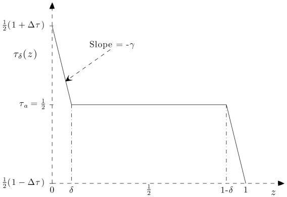
Figure 4: The piecewise linear background profile $\tau_{\delta}(z)$, with $\tau^{\prime}=-\gamma$ in the boundary layer, and $\tau^{\prime}=0$ in the bulk.

From (B.23) we immediately compute $\tau(0)=\tau_{a}+\gamma\delta$, $\tau(1)=\tau_{a}-\gamma\delta$, and so

$$\Delta\tau=\tau(0)-\tau(1)=2\delta\gamma,\qquad\int_{0}^{1}\tau^{\prime 2}\,dz=2\delta\gamma^{2}=\gamma\Delta\tau,$$ (B.24)

where it remains to choose the average $\tau_{a}=\tfrac{1}{2}(\tau(0)+\tau(1))$ and boundary slope $\gamma=-\tau^{\prime}(0)=-\tau^{\prime}(1)$ of the background as functions of $\delta$. Substituting $\Delta\tau=2\delta\gamma$ into (B.5), we obtain the values of $\gamma$ and $\Delta\tau$ (for given $\delta$ and $\eta$) for which $\tau_{\delta}(z)$ defined in (B.23) satisfies the mixed (Robin) thermal BCs:

$$\gamma=\frac{1+2\eta}{2(\delta+\eta)},\qquad\Delta\tau=2\delta\gamma=\frac{\delta(1+2\eta)}{\delta+\eta}.$$ (B.25)

Now using this $\gamma$ in the BC (2.17) written as $\tau(0)=1+\eta+\eta\tau^{\prime}(0)$ for $\eta<\infty$, we find that $\tau_{a}=1/2$, completing the specification of the background $\tau_{\delta}(z)$. (In the fixed flux case $\eta=\infty$, in which the governing equations depend only on temperature gradients, $\tau_{a}$ is arbitrary; for consistency we choose $\tau_{a}=1/2$.)

Substituting (B.24)–(B.25) into (B.19)–(B.20) and simplifying, we now find that the conservative bounds on $\beta$ and $\Delta T$ for fixed Biot number convection with a piecewise linear (pwl) background profile $\tau_{\delta}$ take the concise forms

$$\beta\leq\mathcal{B}_{\mathrm{pwl},\eta}(\delta,b)\equiv\mathcal{B}_{\eta}[\tau_{\delta};b] =1+b\,\frac{1}{2}\,\frac{1-2\delta}{\delta+\eta}=1+b(\gamma-1),$$ (B.26)

$$\Delta T\geq\mathcal{D}_{\mathrm{pwl},\eta}(\delta,b)\equiv\mathcal{D}_{\eta}[\tau_{\delta};b] =1-b\,\eta\,\frac{1-2\delta}{\delta+\eta}=1+b(\Delta\tau-1),$$ (B.27)

corresponding to an upper bound on the Nusselt number of $\mathit{Nu}\leq\mathcal{N}_{\mathrm{pwl},\eta}(\delta,b)\equiv\mathcal{N}_{\eta}[\tau_{\delta};b]=\mathcal{B}_{\mathrm{pwl},\eta}(\delta,b)/\mathcal{D}_{\mathrm{pwl},\eta}(\delta,b)$.

Relation to convection with plates:

The development in this Appendix of a bounding principle for convection with mixed thermal BCs of fixed Biot number $\eta$, applied directly at the fluid boundaries, parallels the calculations in §§ 3.2–5.1 for convection with imperfectly conducting bounding plates.

As discussed in § 5.2, it turns out that the strong admissibility criteria for convection with and without plates coincide, so that the estimates of § 5.3 for verifying strong admissibility for piecewise linear backgrounds also apply to the present mixed BC case. Furthermore, for convection with plates with $\sigma=d/\lambda$, the piecewise linear field $\bar{\tau}_{\delta}(z)$ defined in (5.1) satisfies mixed thermal BCs with Biot number $\eta=\sigma$, and the corresponding bounds on $\mathit{Nu}$ agree. Hence the further derivation of bounds for fixed Biot number BCs can proceed simultaneously with that for convection with bounding plates. Asymptotic bounds for convection with Biot number $\eta$, and equivalently for plates with $\sigma=\eta$, are obtained in § 6, with a discussion of their scaling regimes for increasing $R$.

References

- Ahlers et al. (2009a) Ahlers, G., Funfschilling, D. & Bodenschatz, E. 2009a Transitions in heat transport by turbulent convection at Rayleigh numbers up to . New J. Phys. 11, 123001.
- Ahlers et al. (2009b) Ahlers, G., Grossmann, S. & Lohse, D. 2009b Heat transfer and large scale dynamics in turbulent Rayleigh-Bénard convection. Rev. Mod. Phys. 81, 503–537.
- Amati et al. (2005) Amati, G., Koal, K., Massaioli, F., Sreenivasan, K. R. & Verzicco, R. 2005 Turbulent thermal convection at high Rayleigh numbers for a Boussinesq fluid of constant Prandtl number. Phys. Fluids 17, 121701.
- Balmforth et al. (2006) Balmforth, N. J., Ghadge, S. A., Kettapun, A. & Mandre, S. D. 2006 Bounds on double-diffusive convection. J. Fluid Mech. 569, 29–50.
- Brown et al. (2005) Brown, E., Nikolaenko, A., Funfschilling, D. & Ahlers, G. 2005 Heat transport in turbulent Rayleigh-Bénard convection: Effect of finite top- and bottom-plate conductivities. Phys. Fluids 17, 075108.
- Busse (1969) Busse, F. H. 1969 On Howard’s upper bound for heat transport by turbulent convection. J. Fluid Mech. 37, 457–477.
- Busse & Riahi (1980) Busse, F. H. & Riahi, N. 1980 Nonlinear convection in a layer with nearly insulating boundaries. J. Fluid Mech. 96, 243–256.
- Chapman et al. (1980) Chapman, C. J., Childress, S. & Proctor, M. R. E. 1980 Long wavelength thermal convection between non-conducting boundaries. Earth Planet. Sci. Lett. 51, 362–369.
- Chapman & Proctor (1980) Chapman, C. J. & Proctor, M. R. E. 1980 Nonlinear Rayleigh-Bénard convection between poorly conducting boundaries. J. Fluid Mech. 101 (4), 759–782.
- Chaumat et al. (2002) Chaumat, S., Castaing, B. & Chillà, F. 2002 Rayleigh-Bénard cells: influence of the plates’ properties. In Advances in Turbulence IX, Proceedings of the Ninth European Turbulence Conference (ed. I. P. Castro, P. E. Hancock & T. G. Thomas), pp. 159–162. CIMNe, Barcelona.
- Chavanne et al. (2001) Chavanne, X., Chillà, F., Chabaud, B., Castaing, B. & Hébral, B. 2001 Turbulent Rayleigh-Bénard convection in gaseous and liquid He. Phys. Fluids 13, 1300–1320.
- Chillà et al. (2004) Chillà, F., Rastello, M., Chaumat, S. & Castaing, B. 2004 Ultimate regime in Rayleigh-Bénard convection: The role of plates. Phys. Fluids 16, 2452–2456.
- Constantin & Doering (1996) Constantin, P. & Doering, C. R. 1996 Heat transfer in convective turbulence. Nonlinearity 9, 1049–1060.
- Cross & Hohenberg (1993) Cross, M. & Hohenberg, P. 1993 Pattern formation outside of equilibrium. Rev. Mod. Phys. 65 (3), 851–1112.
- Doering & Constantin (1992) Doering, C. R. & Constantin, P. 1992 Energy dissipation in shear driven turbulence. Phys. Rev. Lett. 69 (11), 1648–1651.
- Doering & Constantin (1996) Doering, C. R. & Constantin, P. 1996 Variational bounds on energy dissipation in incompressible flows. III. Convection. Phys. Rev. E 53 (6), 5957–5981.
- Doering et al. (2006) Doering, C. R., Otto, F. & Reznikoff, M. G. 2006 Bounds on vertical heat transport for infinite-Prandtl-number Rayleigh-Bénard convection. J. Fluid Mech. 560, 229–241.
- Funfschilling et al. (2009) Funfschilling, D., Bodenschatz, E. & Ahlers, G. 2009 Search for the “ultimate state” in turbulent Rayleigh-Bénard convection. Phys. Rev. Lett. 103, 014503.
- Gertsberg & Sivashinsky (1981) Gertsberg, V. L. & Sivashinsky, G. I. 1981 Large cells in nonlinear Rayleigh-Bénard convection. Prog. Theor. Phys. 66, 1219–1229.
- Glazier et al. (1999) Glazier, J. A., Segawa, T., Naert, A. & Sano, M. 1999 Evidence against ‘ultrahard’ thermal turbulence at very high Rayleigh numbers. Nature 398, 307–310.
- Grigné et al. (2007a) Grigné, C., Labrosse, S. & Tackley, P. J. 2007a Convection under a lid of finite conductivity: Heat flux scaling and application to continents. J. Geophys. Res. 112, B08402.
- Grigné et al. (2007b) Grigné, C., Labrosse, S. & Tackley, P. J. 2007b Convection under a lid of finite conductivity in wide aspect ratio models: Effect of continents on the wavelength of mantle flow. J. Geophys. Res. 112, B08403.
- Grossmann & Lohse (2000) Grossmann, S. & Lohse, D. 2000 Scaling in thermal convection: a unifying theory. J. Fluid Mech. 407, 27–56.
- Guillou & Jaupart (1995) Guillou, L. & Jaupart, C. 1995 On the effects of continents on mantle convection. J. Geophys. Res. 100, 24,217–24,238.
- Heslot et al. (1987) Heslot, F., Castaing, B. & Libchaber, A. 1987 Transitions to turbulence in helium gas. Phys. Rev. A 36, 5870–5873.
- Holmedal et al. (2005) Holmedal, B., Tveitereid, M. & Palm, E. 2005 Planform selection in Rayleigh-Bénard convection between finite slabs. J. Fluid Mech. 537, 255–270.
- Hopf (1941) Hopf, E. 1941 Ein allgemeiner Endlichkeitssatz der Hydrodynamik. Math. Ann. 117, 764–775.
- Howard (1963) Howard, L. N. 1963 Heat transport by turbulent convection. J. Fluid Mech. 17, 405–432.
- Hunt et al. (2003) Hunt, J. C. R., Vrieling, A. J., Nieuwstadt, F. T. M. & Fernando, H. J. S. 2003 The influence of the thermal diffusivity of the lower boundary on eddy motion in convection. J. Fluid Mech. 491, 183–205.
- Hurle et al. (1967) Hurle, D. T. J., Jakeman, E. & Pike, E. R. 1967 On the solution of the Benard problem with boundaries of finite conductivity. Proc. R. Soc. London A 296 (1447), 469–475.
- Ierley et al. (2006) Ierley, G. R., Kerswell, R. R. & Plasting, S. C. 2006 Infinite-Prandtl-number convection. Part 2. A singular limit of upper bound theory. J. Fluid Mech. 560, 159–227.
- Jenkins & Proctor (1984) Jenkins, D. R. & Proctor, M. R. E. 1984 The transition from roll to square-cell solutions in Rayleigh-Bénard convection. J. Fluid Mech. 139, 461–471.
- Johnston & Doering (2009) Johnston, H. & Doering, C. R. 2009 A comparison of turbulent thermal convection between conditions of constant temperature and constant flux. Phys. Rev. Lett. 102, 064501.
- Kadanoff (2001) Kadanoff, L. P. 2001 Turbulent heat flow: Structures and scaling. Physics Today pp. 34–39.
- Kerswell (1997) Kerswell, R. R. 1997 Variational bounds on shear-driven turbulence and turbulent Boussinesq convection. Physica D 100, 355–376.
- Kerswell (2001) Kerswell, R. R. 2001 New results in the variational approach to turbulent Boussinesq convection. Phys. Fluids 13 (1), 192–209.
- Kraichnan (1962) Kraichnan, R. H. 1962 Turbulent thermal convection at arbitrary Prandtl number. Phys. Fluids 5, 1374–1389.
- Lenardic & Moresi (2003) Lenardic, A. & Moresi, L. 2003 Thermal convection below a conducting lid of variable extent: Heat flow scaling and two-dimensional, infinite Prandtl number numerical simulations. Phys. Fluids 15, 455–466.
- Malkus (1954) Malkus, M. V. R. 1954 The heat transport and spectrum of thermal turbulence. Proc. Roy. Soc. Lond. A 225, 196–212.
- Nicodemus et al. (1997) Nicodemus, R., Grossmann, S. & Holthaus, M. 1997 Improved variational principle for bounds on energy dissipation in turbulent shear flow. Physica D 101, 178–190.
- Niemela & Sreenivasan (2006a) Niemela, J. J. & Sreenivasan, K. R. 2006a Turbulent convection at high Rayleigh numbers and aspect ratio 4. J. Fluid Mech. 557, 411–422.
- Niemela & Sreenivasan (2006b) Niemela, J. J. & Sreenivasan, K. R. 2006b The use of cryogenic helium for classical turbulence: Promises and hurdles. J. Low Temp. Phys. 143, 163–212.
- Normand et al. (1977) Normand, C., Pomeau, Y. & Velarde, M. G. 1977 Convective instability: A physicist’s approach. Rev. Mod. Phys. 49, 581–624.
- Otero et al. (2004) Otero, J., Dontcheva, L. A., Johnston, H., Worthing, R. A., Kurganov, A., Petrova, G. & Doering, C. R. 2004 High-Rayleigh-number convection in a fluid-saturated porous layer. J. Fluid Mech. 500, 263–281.
- Otero et al. (2002) Otero, J., Wittenberg, R. W., Worthing, R. A. & Doering, C. R. 2002 Bounds on Rayleigh-Bénard convection with an imposed heat flux. J. Fluid Mech. 473, 191–199.
- Plasting & Kerswell (2003) Plasting, S. C. & Kerswell, R. R. 2003 Improved upper bound on the energy dissipation rate in plane Couette flow: the full solution to Busse’s problem and the Constantin-Doering-Hopf problem with one-dimensional background field. J. Fluid Mech. 477, 363–379.
- Procaccia & Sreenivasan (2008) Procaccia, I. & Sreenivasan, K. R. 2008 The state of the art in hydrodynamic turbulence: Past successes and future challenges. Physica D 237, 2167–2183.
- Proctor (1981) Proctor, M. R. E. 1981 Planform selection by finite-amplitude thermal convection between poorly conducting slabs. J. Fluid Mech. 113, 469–485.
- Roche et al. (2005) Roche, P.-E., Gauthier, F., Chabaud, B. & Hébral, B. 2005 Ultimate regime of convection: Robustness to poor thermal reservoirs. Phys. Fluids 17, 115107.
- Siggers et al. (2004) Siggers, J. H., Kerswell, R. R. & Balmforth, N. J. 2004 Bounds on horizontal convection. J. Fluid Mech. 517, 55–70.
- Sparrow et al. (1964) Sparrow, E. M., Goldstein, R. J. & Jonsson, V. K. 1964 Thermal instability in a horizontal fluid layer: effect of boundary conditions and non-linear temperature profile. J. Fluid Mech. 18, 513–528.
- Stevens et al. (2010) Stevens, R. J. A. M., Verzicco, R. & Lohse, D. 2010 Radial boundary layer structure and Nusselt number in Rayleigh-Bénard convection. J. Fluid Mech. 643, 495–507.
- Verzicco (2004) Verzicco, R. 2004 Effects of nonperfect thermal sources in turbulent thermal convection. Phys. Fluids 16, 1965–1979.
- Verzicco & Sreenivasan (2008) Verzicco, R. & Sreenivasan, K. R. 2008 A comparison of turbulent thermal convection between conditions of constant temperature and constant heat flux. J. Fluid Mech. 595, 203–219.
- Westerburg & Busse (2001) Westerburg, M. & Busse, F. H. 2001 Finite-amplitude convection in the presence of finitely conducting boundaries. J. Fluid Mech. 432, 351–367.
- Wittenberg & Gao (2010) Wittenberg, R. W. & Gao, J. 2010 Conservative bounds on Rayleigh-Bénard convection with mixed thermal boundary conditions. To appear in Eur. Phys. J. B.