A multiscale view on inverse statistics and gain/loss asymmetry in financial time series

Abstract

Researchers have studied the first passage time of financial time series and observed that the smallest time interval needed for a stock index to move a given distance is typically shorter for negative than for positive price movements. The same is not observed for the index constituents, the individual stocks. We use the discrete wavelet transform to illustrate that this is a long rather than short time scale phenomenon — if enough low frequency content of the price process is removed, the asymmetry disappears. We also propose a new model, which explain the asymmetry by prolonged, correlated down movements of individual stocks.

1 Introduction

Modelling the statistical properties of financial time series has long been an active area of research, both in the spaces of economics and physics. The traditional object of study has been the returns of various assets, i.e. the size of price movements over fixed time intervals. Inspired by research in the field of turbulence, Simonsen, Jensen and Johansen [8] asked the “inverse” question: what is the smallest time interval needed for an asset to cross a fixed return level $\rho$? Figure 1 shows the distribution of this random variable, the first passage time, for the Dow Jones Industrial Average index, for $\rho=\pm 5\%$. As noted by Jensen, Johansen and Simonsen [5], the most likely first passage time is shorter for $\rho=-5\%$ than for $\rho=5\%$, which they refer to as the gain/loss asymmetry. Intriguingly, the same asymmetry is not observed in the constituents of the index, the individual stocks [6].

One explanation for the gain/loss asymmetry in the index is that occasionally, the stocks move in a highly correlated manner, and that this tend to happen for down movements rather than up movements [3]. To support this view, Donangelo, Jensen, Simonsen and Sneppen [3] proposed the asymmetric synchronous market model, where the log stock prices move like independent random walks for most days, but sometimes move downwards together. This model exhibits gain/loss asymmetry for the index, but not for the individual stocks.

In this paper we investigate on what time scale the gain/loss asymmetry emerges. To this end, we use the discrete wavelet transform and estimate the first passage time for high-pass filtrations of the time series. Apparently, if enough low frequency content is removed, the gain/loss asymmetry disappears — the asymmetry is due to effects on quite long time scales, 64-128 days and longer. Together with the fact that individual stocks do not exhibit gain/loss asymmetry this indicates that the asymmetry is due to prolonged, correlated down-movements of the stock prices. This is contrary to the model from Donangelo et al. [3], where the correlated losses are “local” in time. Indeed, we illustrate that the gain/loss asymmetry in that model emerges on a rather short time scale, which is inconsistent with our empirical findings. Finally, we construct a new model where the gain/loss asymmetry emerges on longer time scales, consistent with the empirical findings.

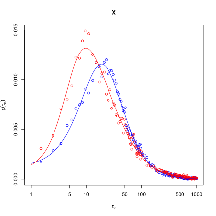
Figure 1: Estimated distribution of the first passage time $\tau_{\rho}$ for the log price of the Dow Jones industrial Average index. The graphs correspond to $\rho=+5\%$ (blue) and $\rho=-5\%$ (red).

2 First passage time on multiple time scales

Throughout this section we let $\{X_{t}\}_{t\geq 0}$ denote the logarithm of a financial time series, for instance the price of a stock index. The first passage time $\tau_{\rho}$ of the level $\rho$ is defined as

$$\tau_{\rho}=\left\{\begin{array}[]{ll}\inf\{s>0;\ X_{t+s}-X_{t}\geq\rho\}&\mbox{if }\rho>0,\\ \inf\{s>0;\ X_{t+s}-X_{t}\leq\rho\}&\mbox{if }\rho<0,\end{array}\right.$$

and is assumed to be independent of $t$. The distribution of $\tau_{\rho}$ is estimated in a straight forward manner from a time series $X=(X_{t_{1}},\ldots,X_{t_{N}})$. Consider $\rho>0$, and let $t_{n+m}$ be the smallest time point such that $X_{t_{n+k}}-X_{t_{n}}\geq\rho$, if such a time point exists. In that case, $t_{n+m}-t_{n}$ is viewed as an observation of $\tau_{\rho}$. (If $\rho<0$, take instead $t_{n+m}$ such that $X_{t_{n+k}}-X_{t_{n}}\leq\rho$.) Running $n$ from $1$ to $N-1$ gives a set of observations from which the distribution of $\tau_{\rho}$ is estimated as the empirical distribution.

Given a time series $X=(X_{t_{1}},\ldots,X_{t_{N}})$, the level-$J$ discrete wavelet transform yields an additive decomposition

$$X=\sum_{j=1}^{J}D_{j}+S_{J},$$

where $D_{j}$ is the $j$:th level detail and $S_{J}$ is the $J$:th level smooth. Essentially, $D_{j}$ is a band-pass filtration and $S_{J}$ is a low-pass filtration of $X$. If $X$ consists of daily observations, then $D_{j}$ contains changes on a time scale of between $2^{j-1}$ and $2^{j}$ days, and $S_{J}$ contains changes on timescales longer than $2^{J}$ days. The signal $R_{J}:=X-S_{J}$ can thus be seen as a “detrended” version of $X$, where the time horizon of the removed trends increases exponentially with $J$.

We considered the time series $X$ of daily observations of the Dow Jones Industrial Average index, henceforth DJIA, and computed the filtered signals $R_{6},R_{8}$ and $R_{10}$ (see Figure 2). We then estimated the distribution of the first passage time for $R_{6},R_{8},R_{10}$, and $X$. Figure 3 show the result: the gain/loss-asymmetry is absent for $R_{6}$, and gradually emerges for $R_{8}$ and $R_{10}$. This indicates that if enough low frequency components of the signal are removed, the gain/loss asymmetry disappears. Since the level $J=6$ corresponds to 32-64 days, the asymmetry appears mainly due to effects on rather long time scales: 64-128 days and longer. The same pattern was observed for other stock indices, like the S&P500 and Nasdaq (not reported).

Figure 2: The log price of the Dow Jones Industrial Average index, $X$, and its high-pass filtrations $R_{6},R_{8}$ and $R_{10}$.

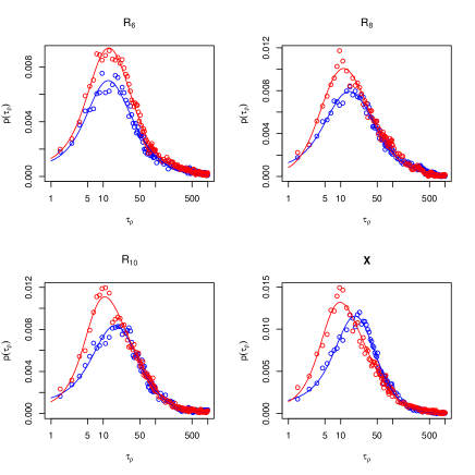
Figure 3: Estimated distribution of the first passage time $\tau_{\rho}$ for $X$, the log price of the Dow Jones Industrial Average index, and its high-pass filtrations $R_{6},R_{8}$ and $R_{10}$. The graphs correspond to $\rho=+5\%$ (blue) and $\rho=-5\%$ (red).

Figure 4 shows the results from the same analysis for the IBM stock price. We see that there is virtually no asymmetry for the IBM stock, at any time scale, which is consistent with the observations from Johansen et al. [6]. We have also confirmed this for several other individual stocks.

In light of the finding that the gain/loss asymmetry in stock indices are due to effects on long rather that short time scales, it is natural to question the structure of the asymmetric synchronous market model (ASMM) given by Donangelo et al. [3]. In that model, the features giving rise to the gain/loss asymmetry by construction takes place on the shortest possible time scale. To see to what extent the gain/loss asymmetry in ASMM resembles that of DJIA when considered on multiple time scales, we performed the analysis for a realization of the model. That is, we let $X$ be a time series generated by ASMM, and estimated the first passage time densities for $R_{6},R_{8},R_{10}$, and $X$. Figure 5 shows the result — the gain/loss symmetry is evidently present already on shorter time scales, for $R_{6}$ and $R_{8}$, which is in contrast with the empirical findings (cf. Figure 3).

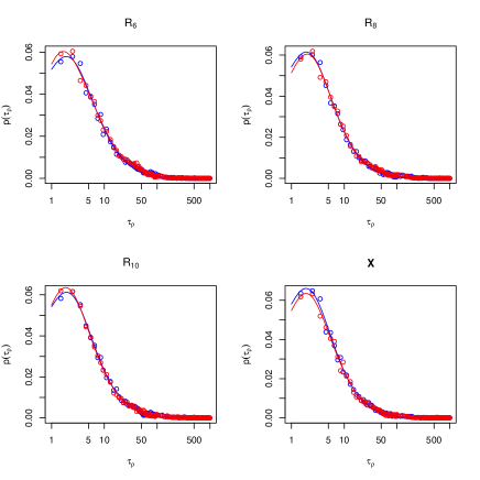
Figure 4: Estimated distribution of the first passage time $\tau_{\rho}$ for $X$, the log price of the IBM stock, and its high-pass filtrations $R_{6},R_{8}$ and $R_{10}$. The graphs correspond to $\rho=+5\%$ (blue) and $\rho=-5\%$ (red).

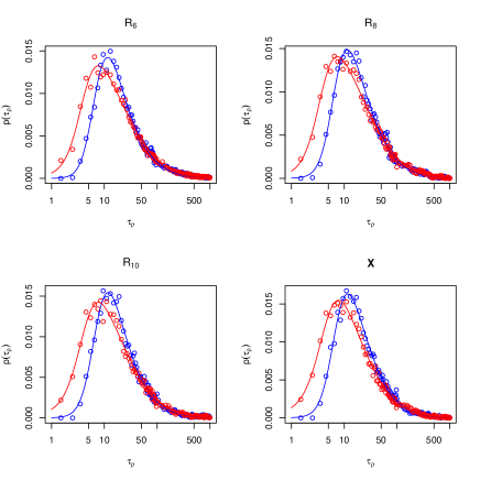
Figure 5: Estimated distribution of the first passage time $\tau_{\rho}$ for $X$, the log price in a realization of ASMM with $N=30$ stocks, and its high-pass filtrations $R_{6},R_{8}$ and $R_{10}$. The graphs correspond to $\rho=5\sigma$ (blue) and $\rho=-5\sigma$ (red).

3 A new model

In this section we propose a new model to remedy the failure of ASMM in reproducing the gain/loss asymmetry when considered on multiple time scales. The new model can be seen as a generalization of ASMM — it has one “regular” state where the stocks move independently, and one “distressed” state where their moves are highly correlated. The most important difference between our model and ASMM is that the market may remain in the distressed state for several days. Conceptually, this is in correspondence with the empirical findings from the previous section, that the gain/loss asymmetry is due to effects on long rather than short time scales.

In the regular state, all stocks follow independent geometric Brownian motions with drifts $\mu_{r}$ and standard deviation $\xi$:

$$S_{i}(t+\Delta t)=S_{i}(t)e^{(\mu_{r}-\frac{\xi^{2}}{2})\Delta t+\xi\sqrt{\Delta t}Z_{i}},$$

where $Z_{i}$, $i=1,\ldots,N$, are independent standard normals. In the distressed state, there is a pronounced negative drift $\mu_{d}<0$, and all the stocks move together:

$$S_{i}(t+1)=S_{i}(t)e^{(\mu_{d}-\frac{\xi^{2}}{2})\Delta t+\xi\sqrt{\Delta t}Z},$$

where $Z$ is standard normal — the single random variable $Z$ drives the price change in all the stocks. For any given day, we consider the possibility of changing states: we let $p_{rd}$ denote the probability of changing from the regular to the distressed state, and let $p_{dr}$ denote the probability of the converse transition. The index is defined by

$$I(t):=\frac{1}{N}\sum_{i=1}^{N}S_{i}(t).$$

Note that ASMM can be seen as a particular case of this model, with $p_{dr}=1$ — the transition from the distressed to the normal state always happens in one day.

We fix the following parameters: $\Delta t=1/250$, $\xi=0.3$, $\mu_{d}=-0.15$, $p_{rd}=1/200$, $p_{dr}=1/25$, and choose the drift $\mu_{r}$ in order to make $\mathbb{E}[(I(t+\Delta t)-I(t))/I(t)]=2.58\cdot 10^{-4}$ (this is the historical daily mean return of DJIA). As above, let $\rho=\pm 5\sigma$, where $\sigma$ denotes the daily standard deviation of the change in $\log(I(t+\Delta t)/I(t))$.

Figure 6 show the estimated first passage density for the index and its high-pass filtrations, for $N=30$ stocks. We see that the multiresolution analysis resembles that of DJIA: the gain/loss asymmetry is absent for $R_{6}$ but emerges for $R_{8}$ and $R_{10}$. Figure 7 show the result from the same analysis but with $N=1$ stock: as expected, there is no gain/loss asymmetry in this case. Again, this is consistent with the empirical findings, that individual stocks do not exhibit gain/loss asymmetry.

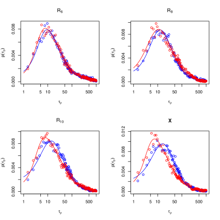
Figure 6: Estimated distribution of the first passage time $\tau_{\rho}$ for $X$, the log price in a realization of our proposed model with $N=30$ stocks, and its high-pass filtrations $R_{6},R_{8}$ and $R_{10}$. The graphs correspond to $\rho=5\sigma$ (blue) and $\rho=-5\sigma$ (red).

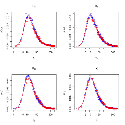
Figure 7: Estimated distribution of the first passage time $\tau_{\rho}$ for $X$, the log price in a realization of our proposed model with $N=1$ stock, and its high-pass filtrations $R_{6},R_{8}$ and $R_{10}$. The graphs correspond to $\rho=5\sigma$ (blue) and $\rho=-5\sigma$ (red).

4 Conclusion

Using wavelet multiresolution analysis, we have shown that the so called gain/loss asymmetry observed in stock indices is due to effects on long rather than short time scales — the asymmetry disappears if enough low frequency content is removed from the signal. Moreover, inspired by the asymmetric synchronous market model, we proposed a new model featuring prolonged periods of correlated down movements of the index constituents that qualitatively reproduces the asymmetry.

According to our new model, the stock market occasionally enters a distressed state of correlated down movements and stays there for a prolonged period of time, expected to last $1/p_{dr}$ days. In the future, we would like to investigate whether it is possible to estimate this quantity from data by comparing empirical first passage time distributions to the distributions implied by the model, in effect “calibrating” the model. We are intrigued by the question of how such information may relate to the so called Heterogeneous Market Hypothesis [1] — that is, that various participants in the market have different time horizons and dealing frequencies. The wavelet multiscale decomposition of the signal could potentially be used be to investigate the emergence of the gain/loss asymmetry even further. For instance, what happens if the signal is band-pass instead of high-pass filtered — is it possible to pinpoint the time scale of the origin of the asymmetry?

References

References

- [1] Michel M. Dacorogna, Ramazan Gencay, Ulrich Muller, Richard B. Olsen, and Olivier V. Pictet. An introduction to high-frequency finance. Academic Press, 2001.
- [2] I. Daubechies. Ten Lectures on Wavelets. SIAM, 1992.
- [3] Raul Donangelo, Mogens H. Jensen, Ingve Simonsen, and Kim Sneppen. Synchronization model for stock market asymmetry. Jornal of Statistical Mechanics, 2006.
- [4] Ramazan Gencay, Faruk Selcuk, and Brandon Whitcher. An introduction to wavelets and other filtering methods in finance and economics. Academic Press, 2002.
- [5] Mogens H. Jensen, Anders Johansen, and Ingve Simonsen. Inverse fractal statistics in turbulence and finanace. International Journal of Modern Physics B, 2003.
- [6] Anders Johansen, Mogens H. Jensen, and Ingve Simonsen. Inverse statistics for stocks and markets. Working paper, 2005.
- [7] Donald B. Percival and Andrew T. Walden. Wavelet methods for time series analysis. Camebridge University Press, 2002.
- [8] Ingve Simonsen, Mogens H. Jensen, and Anders Johansen. Optimal investment horizons. European Physical Journal B, 2002.