The chromospherically active binary star EI Eridani

Abstract

Data from 11 years of continuous spectroscopic observations of the active RS CVn-type binary star EI Eridani – gained at NSO/McMath-Pierce, KPNO/Coudé Feed and during the MUSICOS 98 campaign – were used to obtain 34 Doppler maps in three spectroscopic lines for 32 epochs, 28 of which are independent of each other. Various parameters are extracted from our Doppler maps: average temperature, fractional spottedness, and longitudinal and latitudinal spot-occurrence functions. We find that none of these parameters show a distinct variation nor a correlation with the proposed activity cycle as seen from photometric long-term observations. This suggests that the photometric brightness cycle may not necessarily be due to just a cool spot cycle. The general morphology of the spot pattern remains persistent over the whole period of 11 years. A large cap-like polar spot was recovered from all our images. A high degree of variable activity was noticed near latitudes of $\approx$60–70^∘ where the appendages of the polar spot emerged and dissolved.

1 Introduction

Our Sun exhibits cyclic behaviour which can be seen in its spectral output as well as in its spot coverage (Willson & Mordvinov 2003). Apart from the commonly known 11-years Sunspot cycle, our Sun shows an 80 years long so-called Gleissberg cycle and an 200–300 years long pseudo-cycle (Wolf, Spörer, Maunder). Even longer cycles or variations are seen, and there is evidence that periods of cyclic behaviour alternate with times of constant, very low activity (e.g. Maunder minimum). Solar-type G and K stars can exhibit the same solar-like cycles in their photospheric output as originally discovered from their chromospheric Ca ii H & K emission (Baliunas & Soon 1995; Gray et al. 1996). However, a photosphere-chromosphere correlation cannot be easily reproduced for evolved G and K stars (Choi et al. 1995; Frasca et al. 2005). Long-term changes in the mean brightness of RS CVn stars are therefore not a straightforward tool for investigating spot cycles similar to the Sun’s 11-year cycle. From what we know from our Sun, we would expect an activity cycle from Ca ii H & K to be accompanied by a spot cycle.

Several groups began long-term Doppler-imaging studies on a few selected active stars (that usually consist of one or a few images per year, i.e. per observing season): Korhonen et al. (2007, FK Com, 24 maps from 1993 to 2003), Vogt et al. (1999, HR 1099 = V711 Tau, 23 maps from 1981 to 1992), Berdyugina et al. (1998, II Peg, 9 maps from 1992 to 1996; and 2001, LQ Hya, 9 maps from 1993 to 1999), Oláh et al. (2002b, UZ Lib, 8 maps from 1994 to 2000), Marsden et al. (2007, IM Peg, 31 maps from 2003 to 2005), Donati et al. (2003, AB Dor, LQ Hya, HR 1099) and others. All of them are active stars and most of them are close binaries with their rotation period usually spun up by tidal forces. However, so far only one star, HR 1099 (Vogt & Hatzes 1996; Strassmeier & Bartus 2000), has been observed over a sufficiently long time span to cover a complete activity cycle with Doppler maps.

EI Eridani = HD 26337 (G5 iv, $P_{\mbox{\scriptsize rot}}\ =1.947$ days, $V$ = 7.1 mag, $v\sin i=51$ $\mathrm{km\,s}^{-1}$, SB1) was one of the first stars being Doppler imaged. Its spot distribution has been monitored since 1984. Long-term photometric observations revealed large brightness variations which seem to be cyclic and were first supposed to resemble a solar-like 11 years cycle but appear to be more complex as observations continue. Within the first 16 years of photospheric observations, EI Eri gave the impression of a cycle of similar length to the solar cycle: Strassmeier et al. (1997) calculated a length of $11\pm 1$ years. Observations in the following years did not confirm this cycle as they did not meet the anticipated decline of brightness. Berdyugina & Tuominen (1998) estimated a 9-year periodicity from the positions of active regions. They did not discuss a possible change in the level of spottedness itself, though. Oláh et al. (2000) favoured a length of 16.2 years on a time base of 18.5 years and quote a significant remaining period of 2.4 years. Adding four more years of data, the preferred cycle length was back to 12.2 years (see Oláh & Strassmeier 2002). Most recent calculations, comprising an observed time interval of 28 years, state a long cycle of about 14 years with variable amplitude and two short cycles of about 2.9–3.1 years and 4.1–4.9 years (Oláh et al. 2009).

The present program intends to review all available Doppler maps of EI Eri and to possibly link any long-term evolution of the spot distribution to the photometric variations.

2 Doppler imaging of EI Eridani

With its large rotational velocity and an intermediate inclination, EI Eri is, as Fekel et al. (1987) already noted, an ideal candidate for Doppler imaging (hereafter “DI”). Consequently, EI Eri has been a prime target since the first application of this technique to spotted late-type stars in 1982. Doppler maps can be found in Strassmeier (1990, epoch 1987), Strassmeier et al. (1991, epoch 1988; investigation of different DI techniques), and for the 1984-87 period, in Hatzes & Vogt (1992). O’Neal et al. (1996) determined spot covering factors between 16% and 37%.

The data used for producing the maps presented in this paper were obtained at NSO McMath-Pierce during seven years of our long term synoptic observations (1988–1995; 19 maps) and one dedicated visitor observing run in 1996 (three independent maps), several dedicated KPNO/Coudé feed visitor observing runs in 1995, 1996 and 1997 (the latter with three independent maps) and participation in the MUSICOS 1998 observing campaign (three independent maps). The total covered time period streches from 1988 to 1998 (eleven observing seasons). A detailed description of the NSO and KPNO observations and the obtained data was given in Washuettl et al. (2008, hereafter paper I). The observations and data from the MUSICOS 98 campaign will be presented in a forthcoming paper (Washuettl et al. 2009) which will also address the question of differential rotation. Doppler imaging suggests abundances of $-6.3$ dex (Ca) and $-5.5$ dex which are smaller than solar by $-0.6$ dex (Ca) and $-1.1$ dex (see below).

Knowledge of the precise stellar parameters is essential for obtaining good-quality Doppler maps. Parameters like temperature, rotational velocity, luminosity, radius, orbital inclination, mass, period and orbital parameters were already investigated in paper I. Additionally, several specific Doppler-imaging parameters were improved by producing a series of test reconstructions: stellar inclination, differential rotation, rotational velocity, gravity, temperature, abundances, macro and micro turbulence, line blends and transition probabilities. Nomalized $\chi^{2}$ distributions for these parameters which allow to find or improve the parameter value were presented in Washuettl (2004). For a list of DI-relevant parameters, see Table 1. Further astrophysical parameters are listed in paper I, Table 5.

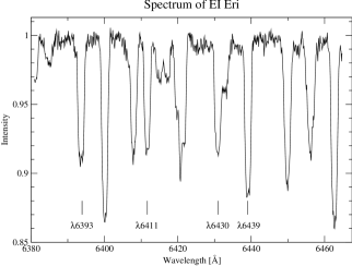
Figure 1: Typical spectrum of EI Eri with the four mapping lines $\lambda$6393, $\lambda$6411, $\lambda$6430 and $\lambda$6439.

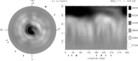
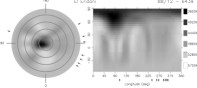
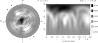
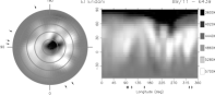
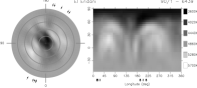
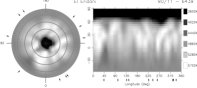
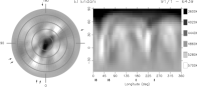
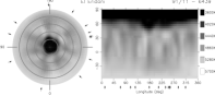
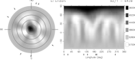
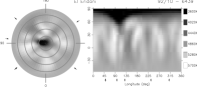
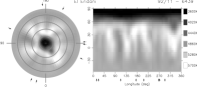
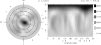
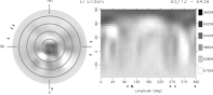
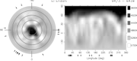
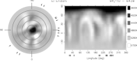
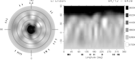
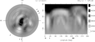
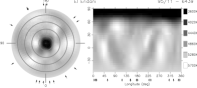
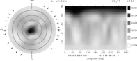
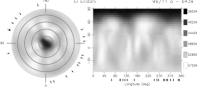
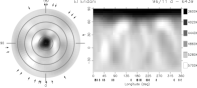
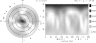
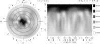
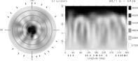
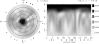
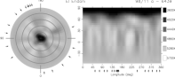
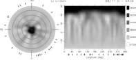
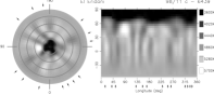
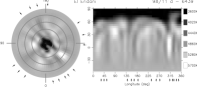
Figure 2: Comparison of all Doppler images from the Ca i 6439 line, consisting of pole-on view (left part), with dark, solid circles drawn at equally spaced intervals of 30^∘ down to a latitude of -30^∘; and pseudo-Mercator projection (right part), from latitude -56^∘ to +90^∘. The phases of the observations are marked by arrows around and below the maps, respectively.

Table 1: Values used as input parameters for the Doppler imaging code TempMap.

Parameter	Value
$P_{\rm phot}=P_{\rm rot}$	1.9472324
T${}_{\rm 0,phot}=$T0,rot	2448054.7109
$\gamma$	21.64 $\mathrm{km\,s}^{-1}$
K1	26.83 $\mathrm{km\,s}^{-1}$
$e$ (eccentricity)	0 (adopted)
$T_{\rm phot}$	5500 K
$T_{\rm max}$	6000 K
$v\sin i$	51.0 $\mathrm{km\,s}^{-1}$
Inclination $i$	56.0∘
$\log g$	3.5
Micro turbulence $\xi$	2.0 $\mathrm{km\,s}^{-1}$
Macro turbulence $\zeta_{\rm r}=\zeta_{\rm t}$	4.0 $\mathrm{km\,s}^{-1}$
Regularisation	Maximum Entropy
Weight of phot. data	0.1
$\log[Ca]$ abundance	$-6.3$ (0.6 dex below solar)
$\log[Fe]$ abundance	$-5.5$ (1.1 dex below solar)

For DI, it is important to obtain high signal-to-noise ratios (S/N $\geq$ 200) at moderate to high spectral resolution ($\lambda$/$\Delta\lambda\ \approx$ 30–40 000). The wavelength region around 6420 Å provides up to four relatively unblended lines usable for DI: Ca I 6439, Fe I 6430, Fe I 6411, and Fe I 6393 and was therefore chosen for the single-order spectrographs available at the McMath-Pierce and Coudé feed telescope. An example spectrum is shown in Fig. 1.

EI Eri’s unfortunate rotational period of 1.947 days is almost an integer multiple of the day/night cycle. As a consequence, one ideally needs 20 nights of continuous observations from a single observing site in order to achieve perfect phase coverage. In practice, 14 consecutive nights are sufficient to give a good-quality Doppler image. No correction for the contribution of the companion star had to be adopted as EI Eri is a single-lined spectroscopic binary. The time resolution of consecutive spectra was 2700 – 3600 s, corresponding to a spot motion of 6 – 8^∘ in longitude on the central meridian of the stellar surface or 5.2 – 6.9 $\mathrm{km\,s}^{-1}$ (0.11 – 0.15 Å) in the spectral line profile. This is still within one resolution element across the broadened line profile: With a typical resolving power of 24 000 – 36 000 ($\lambda/\Delta\lambda$), we achieve 8 – 12 resolution elements across the stellar disk, which corresponds to a velocity resolution of 8.3 – 12.5 $\mathrm{km\,s}^{-1}$ (0.18 – 0.27 Å) and a spatial resolution along the equator at the stellar meridian of approximately 10–14^∘. The orbital smearing accounts to 2.7 – 3.6 $\mathrm{km\,s}^{-1}$ (0.06 – 0.08 Å). We therefore extended our integration limit to 60 minutes.

For the maps presented in this investigation, we apply the Doppler-imaging code TempMap by John Rice – as described by Rice et al. (1989) and reviewed by Piskunov & Rice (1993), Rice (1996) and, most recently, by Rice (2002). All maps were plotted using the same temperature scale from 3600 to 5500 K. The spot temperature was determined by Strassmeier (1990) using standardised $V$ and $R$ photometry and the Barnes-Evans relation (Barnes et al. 1978). He gives a temperature difference (star minus spot) of $1860\pm 400$ K and, with $T_{\mbox{\scriptsize star}}=5460$ K, yields an effective spot temperature of $3600\pm 400$ K. O’Neal et al. (1996) derived spot temperatures by using the 7055 and 8860 Å bands of the titanium oxide molecule and determined, assuming a photospheric value of $T_{\mbox{\scriptsize phot}}=5600$ K, a value of $T_{\mbox{\scriptsize spot}}=3700\pm 200$ K which was confirmed by O’Neal et al. (1998). In practice, the spot temperature is automatically chosen by TempMap and reaches down to 3600 K.

All 30 independent maps for the $\lambda$6439 line are shown in Fig. 2. Like most maps, it resembles a steady pattern: an asymmetric polar spot is escorted by several small low-latitude features. In some cases, spots slightly warmer ($\approx$200 K) than the photosphere occur. These are likely artifacts which are produced by the Doppler imaging code due to, firstly, the use of differential photometry instead of absolutely calibrated photometry and, secondly, due to external uncertainties in the spectra (see Rice & Strassmeier 2000). Lower metallicity values lessen the appearance of artifical hot spots. Therefore, we assume the high divergence of the Fe abundance from the solar case of $-1.1$ dex to be overdone and favour a more modest value of around $-0.5$ dex. This value is in better agreement with the evolutionary tracks by Pietrinferni et al. (2004, see paper I) and is also supported by Nordström et al. (2004). However, recomputing the Fe Doppler maps with the more modest value of $-0.5$ dex does not alter the surface structure as such but only increases the temperature of the artificial hot spots. Therefore, we used the lower metallicity value of $-1.1$ dex for computation of the Fe maps in order to improve their comparability.

3 Analysis and parameterization of Doppler maps

The spectroscopic data were inverted into a series of Doppler images spanning 11 years and amounted to a total of about 100 images for up to 28 independent epochs (34 images in $\lambda$6439, 30 in $\lambda$6430 and 25 in $\lambda$6411 and a few in $\lambda$6393). Mean separation in time between two independent maps is 141 days, minimum and maximum separation is 3 (overlapping) and 382 days, respectively.

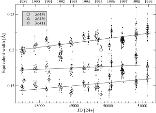
Figure 3: Equivalent widths for the three mapping lines at all epochs. The large open symbols are the mean values for the data used in the respective Doppler maps, the small symbols denote the individual spectra. The black lines denote linear fits for each mapping line. The corresponding values of the fits are listed in Tab. 3.

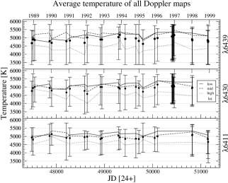
Figure 4: Temperature range for all Doppler maps. Filled circles give the overall average of the respective map, bars denote the minimum and maximum temperature. The solid lines are the low-latitude averages (-55^∘ – 0^∘), the dashed lines the mid-latitude averages (0^∘ – 45^∘), and the dotted lines the high-latitude averages (45^∘ – 90^∘).

Apart from tagging preferred spot locations, we extract several parameters from the Doppler maps and carry out statistical evaluations to see if there are any trends in the temperature distribution or even correlations with the proposed activity cycle (see Fig. 2c in Oláh & Strassmeier 2002, and Fig. 7 in this paper).

3.1 Line equivalent widths

Fig. 3 shows the equivalent widths (EW) for each mapping line (small symbols) as well as the average EW (big symbols) for each set of observations. A possible trend is the linear increase of the EW during the course of the eleven years of observation. This trend is seen with almost the same amount of 11.2 and 11.3% (2.4 and 1.7$\sigma$) in the high-quality line $\lambda$6439 and the mid-quality line $\lambda$6411, but only 4% (0.8$\sigma$) in the poor-quality $\lambda$6430 line (see Tab. 3). If real, this could be suggestive of an increasing chromospheric contribution from a magnetic cycle with a period much longer than our observational coverage.

Table 2: Increase of equivalent width, from Fig. 3.

Wavelength	$\lambda$6439	$\lambda$6430	$\lambda$6411
Initial value (fit) [Å]	0.201	0.172	0.143
Final value (fit) [Å]	0.223	0.179	0.159
Increase value [Å]	0.022	0.007	0.016
Increase percentage	11.2 %	4.2 %	11.3 %
Standard dev.	0.009	0.009	0.010
Incr. value/Std. dev.	2.4$\sigma$	0.8$\sigma$	1.7$\sigma$

Table 3: Increase of fractional spottedness, from Fig. 6. Units are percentage points.

Wavelength	$\lambda$6439	$\lambda$6430	$\lambda$6411
Initial value (fit)	11.2	15.0	16.6
Final value (fit)	12.6	21.5	18.9
Increase value]	1.47	6.43	2.24
Increase percentage	13.2 %	42.7 %	13.5 %
Standard dev.	2.7	3.4	1.8
Incr. value/Std. dev.	0.54$\sigma$	1.9$\sigma$	1.2$\sigma$

3.2 Surface temperature

Fig. 4 shows the progression of the average temperature for all Doppler maps from 1989 to 1999, distinguished for each mapping line. The filled circles are the overall temperature averages of the corresponding Doppler maps, the bars in the axis of ordinates denote the minimum and maximum temperature, the respective upper solid line is the temperature average of the low-latitude band, the dotted line that of the mid-latitude band and the lower solid line that of the high-latitude band. The low, mid, high-latitude bands run from $-$55^∘ to 0^∘, from 0^∘ to 45^∘, and from 45^∘ to 90^∘, respectively (smaller latitudes are not seen as they are tilted out of sight due to the stellar inclination). Temperature variations are noticed but not resembled in all spectral lines at the same time and therefore are likely not real. However, there seems to be a spot maximum (corresponding to a minimum in temperature) in the high-latitude band in 1992 and again in around 1995, seen in $\lambda$6439 and $\lambda$6430. Overall, no pronounced correlation with the photometric variation is evident though. Systematically wrong input values for the line-profile computations can lead to spurious variations in the overall temperature, e.g. caused by artificial hot spots. In order to account for possible misfits, the latitude-dependent temperature averages were normalized by the respective total average temperature. More clearly, we now perceive the temperature decrease in high latitudes in 1992 (in the $\lambda$6439 and $\lambda$6430 line) which corresponds to an increase in the low-latitude band. We also see a clear overall negative correlation between temperature variations in the high and the low latitude bands. However, as in the pre-normalized case, all variations seen are not resembled in all spectral lines and therefore are likely not real. Above all, we do not perceive an apparent correlation between temperature and any other of the parameters derived from the Doppler maps. In particular, no correlation with the long-term photometric variations as seen in Fig. 7 and, more clearly, in Oláh & Strassmeier (2002, Fig. 2c), is evident.

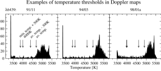
Figure 5: Temperature threshold definitions for three examples of temperature distributions in our Doppler maps (Nov. 1993, Mar. 1994, Jan. 1998). The arrows represent several threshold definitions for calculating the fractional spottedness in Fig. 6.

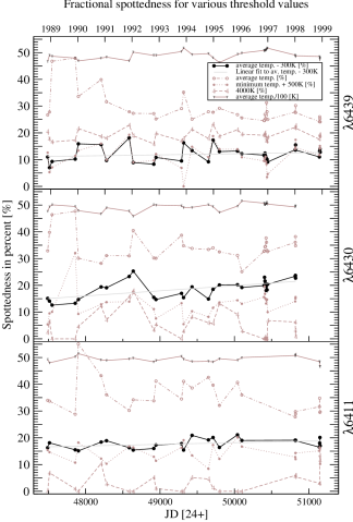
Figure 6: Fractional spottedness in % of the entire sphere for all Doppler maps as a function of time and various threshhold values (explained in the insert). The solid black line with filled circles, i.e. the average temperature minus 300 K (solid black line), gives the most consistent results. The grey line denotes the correponding linear fit, see Tab. 6. For comparison, the average temperatur (divided by 100) is plotted.

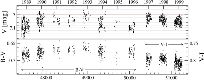
Figure 7: Photometric data for the time coverage of our Doppler maps from Oláh & Strassmeier (2002, for the complete data set, see their Fig. 2c).

3.3 Fractional spottedness

We define a temperature threshold value and count the number of pixels on the star’s surface with temperatures below this threshold and relate it to the total number of surface pixels. Several options for defining a threshold are presented in Fig. 5 which displays three examples of temperature distributions from the $\lambda$6439 line. First, the overall temperature average is established, which usually sits at the lower edge of the photospheric temperature domain (5000–5500K). Its location is, however, so close to the edge that, as a second threshold option, a reduction of the temperature average by a fixed value of 300 K seems advisable. Alternatively, we use the minimum value increased by 500 K and an arbitrarily fixed value of 4000 K as threshold temperatures. All temperature values smaller than the respective threshold temperature provide us with a fraction value which is translated to spottedness in percent. The results are shown in Fig. 6. The threshold based on the average temperature is, as presumed, too close to the photospheric-temperature bulge and sometimes exhibits large increases (around 1990 which is not seen in any of the other curves), induced by the scattering of the photospheric range. The minimum temperature, increased by a specific value, seems to be valuable but sometimes exhibits large deviations which are not resembled in any of the other mapping lines. Overall, we conclude that the average temperature decreased by 300 K gives the most reliable threshold as it lies well between the photospheric and the spot-temperature bulge.

Concentrating on the solid black line with filled circles (Fig. 6), we notice an increase in spottedness in 1992 of 10 percentage points in $\lambda$6439 (according to a factor 2), also seen in the $\lambda$6430 map and another small increase (4 to 6 percentage points) in 1995, mainly in the $\lambda$6439 map. We may compare these results with spot-filling factors derived from TiO band modelling. Solanki & Unruh (2004) list filling factors of EI Eri (as obtained from O’Neal et al. 1998) for the epochs 1992Mar (total 25% / minimum 11%), 1995Jan (13%/5%) and 1995Dec (13%/5%). These values coincide with the increase seen in $\lambda$6430 in the map 1992Jan as compared to 1995Dec but not to the same extent. However, this relation is not seen at all in $\lambda$6439 and $\lambda$6411. Overall, no systematic changes are evident and, above all, no correlation with the photometric long-term trend is seen.

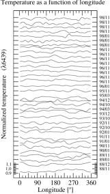
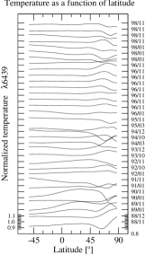
Figure 8: Temporal variations of surface temperature as a function of longitude (left panel) and latitude (right panel). Each function is normalized by the average of all functions and shifted by 0.1 for better viewing. To the right, year and month of observation is unscrambled. The overall temperature profile shows only small and uniform variations. The largest variations are found at high latitudes (65 – 80^∘), as also seen in Fig. 11 (bottom panel).

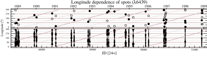
Figure 9: The upper panel gives the longitude of the strongest (filled circles) and second strongest (if existent; open circles) polar appendage for each map. The tilted lines denote the suggested drifting active longitudes. Primary active longitudes are shown as solid lines, secondary active longitudes (on the opposite side of the star) as dotted lines. Lower panel: Longitudinal spot-occurrence functions. The black areas represent average temperature as a function of longitude, normalized by its respective maximum average temperature. A broader area denotes lower average temperature (corresponding to stronger spottedness) at the respective longitude. Overlapping epochs were omitted.

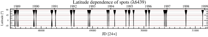
Figure 10: Latitudinal spot-occurrence functions. The black areas mark averaged temperatures as a function of latitude. See Fig. 9b for further description. This display mode is useful for comparing observational results with the theoretical spot-probability functions presented by Granzer et al. (2000).

3.4 Spot occurence functions

Fig. 8 shows for all Doppler maps of the $\lambda$6439 line the temperature distribution as a function of stellar longitude (left) and latitude (right). Starting from 11/1988 on top, each map is shifted by $-$100 K for better viewing. Overall, we cannot determine any preferred surface positions of spots on EI Eridani (apart from the polar cap as such) which is also demonstrated by the “grand average Doppler map”, an average of all available Doppler maps from 1988 through 1998 (Fig. 11). Does this implicate that there are no preferred longitudes at all? This would be in contradiction to what was published by Berdyugina & Tuominen (1998). Their photometry showed active longitudes which were not synchronized with the orbital motion and were shifted by one orbital phase in about 2.7 years together with switching primary and secondary minima after 9 years (flip-flop). Fig. 9 allows a more detailed look at the spot occurrences as a function of stellar longitude. The functions are the same as in Fig. 8 (left) but are plotted as two mirrored contours filled in black, after normalization by their respective maximum temperature (“spot-occurrence function”). A large width denotes lower average temperature and therefore stronger spottedness. The uppermost panel shows the latitudinal locations of the strongest and the second strongest polar appendage as inspected by eye. For the years 1989 till 1994, we see a possible correlation of the longitudinal occurrences of polar appendages, showing a systematic drift towards higher longitudes, i.e. later orbital phase, indicated by solid (primary maxima) and dotted (secondary maxima) grey lines. The shift amounts to 360^∘ after about 3 years which is very similar to the 2.7 years found by Berdyugina & Tuominen (1998). Assuming a switch between primary and secondary minima to occur around 1994 (as proposed by Berdyugina & Tuominen 1998), we reverse the solid and dotted lines at 1994.4 in Fig. 9 (uppermost panel) and see that the continuation from 1994 onwards follows roughly this pattern. The active longitudes noticed in Fig. 9, uppermost panel, are not clearly resembled by the average-temperature functions shown in the lower panels of the same figure (which give an average of each longitude, from $-i$ to 90^∘ latitude). Thus, we conclude that the longitudinal migration is mainly caused by the polar appendages. The latitudinal region of the polar appendages is also the most active area on EI Eri, as revealed by the long-term sigma maps (see Fig. 11 bottom).

Fig. 10 shows the temperature averaged along latitudes. Clearly, the polar cap dominates the surface maps. Compare these results with the diagrams presented by Granzer et al. (2000, Fig. 4). They are similar only to Granzer’s 0.4 $\mathrm{M}_{\mathrm{\odot}}$ cases, and no theoretically predicted spot-probability functions are available yet for giant stars (the results from Granzer et al. are for ZAMS stars).

The lower panel of Fig. 11 shows the respective sigma map of a combination of all maps from 1988–1998 for the $\lambda$6439 line. Clearly, the most and strongest variations are found in the appendices of the polar cap at a latitude of 60^∘ – 75^∘. Nevertheless, as demonstrated by Fig. 10, the extent of the polar cap remains very stable and ends, without exception, at $\approx$50^∘. The polar cap is present in all maps. If the polar cap would vanish for a certain epoch, we would expect the respective line profiles to be more pointed, i.e. less shallow. While all averaged profiles are very homogeneous, a few deviate slightly in line depth. This behaviour is, however, not followed in all three mapping lines simultaneously and is therefore likely due to noise. In fact, none of the extracted parameters exhibits a clear systematic variation in all three mapping lines.

4 Discussion

Our long-term DI study revealed that the brightness variations (exhibiting a period of roughly 12 years) are not resembled by any of the parameters extracted from our Doppler maps nor by the directly measured line equivalent widths. This is in contrast to the solar analog where the total spottedness varies with the activity cycle. Thus, we are asked to explain what exactly causes the long-term variations of the mean brightness and why are these variations not reflected in our Doppler maps.

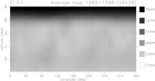
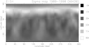
Figure 11: Top: the grand average Doppler map for 1988–1998 ($\lambda$6439). No preferred longitudes in the orbital reference frame are seen. Bottom: Residual map for 1988–1998 ($\lambda$6439).

4.1 Short-term variations

The photometric amplitude varies such that at the begin of the photometric minima in 1984/85, as well as in 1995/96, the amplitude was smallest and turned largest shortly thereafter. A clear correlation with the long-term trend is not obvious (see Fig. 2c in Oláh & Strassmeier 2002, left upper panel). These short-term brightness variations are assumed to be caused by the same spots moving across the visible disk of the star. However, differences in the amplitude of those variations do not necessarily reflect a larger or a smaller number of spots or spottedness. They can also be a sign of a homogeneous or otherwise a concentrated spot distribution on the star’s surface. However, the short-term brightness changes, if caused by spots, should be directly related to the longitude functions in Fig. 9, and should therefore be seen. Most likely, the brightness changes are only caused by those parts of the stellar surface that are not circumpolar. Therefore, we recreated the plot displaying the longitudinal spot-occurrence functions with the high latitudes ( $90\hbox{${}^{\circ}$}-i$ ) excluded. However, a relationship with the brightness variation is still not obvious. After all, for epochs with a small number of photometric data points, the disadvantageous rotational period of almost two days may give an explanation: most photometric data of EI Eri were collected by automatic telescopes which normally execute the same targets every night. This brings about a similar time of observation of a specific target for each night and, in the case of EI Eridani, a similar orbital epoch which will, for a small data sample, mimic smaller photometric amplitudes.

4.2 Long-term variations

A decrease or increase in total brightness – if caused by a larger spottedness or, like on the Sun, by a higher faculae emission – should accordingly be reflected by the spottedness as extracted from the Doppler maps, and thereby also by the average temperature and the equivalent width. However, none of it is the case with EI Eri. One possible explanation is that small inaccuracies in the normalization of the spectra (continuum fitting) could potentially influence the temperature span and thereby introduce noise. Most likely though is that the cyclic brightness variation is caused by a fluctuation of small unresolved spots while the fractional coverage of large-scale spots remains basically constant. Doppler images do a good job in catching starspots that significantly modulate the line profile, but it is extremely difficult to detect a background of small starspots evenly distributed over the stellar surface. Jeffers et al. (2006) obtained spectrophotometric eclipse light curves with HST/STIS and mapped the primary F9 component of the F9V+K4V-IV binary SV Cam. They found that the observed surface flux from the eclipsed low-latitude regions of the F9 primary was 30% lower than what is predicted from model atmospheres and the Hipparcos parallax. This could be explained only if there is about a third of the eclipsed region covered with unresolved cool starspots. Even if this “dark” spot component is assumed to also exist over the rest of the surface, a huge cap-like polar spot down to a latitude of 48^∘ was required in order to fit the eclipse light curves. Solanki & Unruh (2004) found that even for heavily spotted (hypothetical) stars, a large fraction of the spots are smaller than the current resolution limit of Doppler images. Thus, it is possible that a substantial part of the spot coverage is not resembled by our measurements of fractional spottedness (as presented in Fig. 6). Spot covering fractions can also be derived from TiO band modelling, a method that does not suffer from the resolution limitation. It would therefore be essential to monitor and compare fractional spottedness as derived from DI with TiO filling factors. However, Berdyugina (2002) obtained filling factors for the RS CVn system II Peg that agree with the corresponding Doppler images without requiring additional (unresolved) starspots. As a final alternative, we could only assume that the long-term variation of the total mean brightness is not caused by the degree of spottedness. In this case, it would be questionable in what way the photometric cycle corresponds to a magnetic cycle.

4.3 Comparison with the Sun

On the Sun, the solar cycle is visible not only in the visual brightness (see e.g. Willson & Mordvinov 2003) but also in many other tracers including total irradiance, radio and total magnetic flux, Ca ii H & K  emission, in magnetic features like sunspots, and others (see Harvey & White 1999). The sunspot number, though, is the most prominent one. Most indices vary roughly in phase with the sunspot number. However, the modulation amplitude varies widely between different indices. In visible light, the amplitude is marginal and vague, and most likely not obvious to a casual observer.

The sunspot maximum correlates with a maximum in total irradiance/brightness, Ca ii H & K core emission and total magnetic flux (Harvey & White 1999; Radick et al. 1998). Thus, the Sun is brighter during sunspot maximum which is caused by the dominating emission from faculae. This behaviour is also found on other old stars (Radick et al. 1998). Both, the Sun and EI Eri, tend to become bluer as they get brighter, which suggests that EI Eri might exhibit a higher level of faculae emission during activity (i.e. photometric) maximum. On the Sun, however, the emergence of faculae is usually associated with spots.

A model presented by Solanki & Unruh (1998) indicates that the radiative properties of magnetic features on the solar surface (i.e. faculae and sunspots) provide the dominant contribution to irradiance variations on a solar-cycle time-scale, suggesting that such features are also responsible for the visual brightness variations on EI Eri. However, the total irradiance variations seem to be strongly dependent on the inclination angle of the star and, for the Sun, could increase by a factor exceeding 6 when viewed from a heliographic latitude of 60^∘(see Radick et al. 1998). Possibly, the variations in total spottedness on EI Eri are minute and not resolved by our Doppler images while the accompanying faculae could have an enhanced effect on the brightness and photometric colour.

4.4 Comparison with other stars

The surprise that the proposed photometric cycle does not have a corresponding spot or magnetic cycle might get support by results from other stars. Donati et al. (2003) presented long-term magnetic surface images for the young K dwarfs AB Doradus and LQ Hydrae and for the RS CVn-type K1 subgiant HR 1099 and found that large regions with predominantly azimuthal magnetic fields are continuously present at the surface of these stars. Long-term structural changes take place but reflect no more than the limited lifetime of the corresponding surface structures. An active longitude is not confirmed on HR 1099. Furthermore, no clear secular change is detected in the axisymmetric component of the magnetic field and in particular, no global polarity switch was observed in the field ring pattern of HR 1099, nor in the high-latitude azimuthal-field ring of AB Dor. Petit et al. (2004) report that, on HR 1099, the small-scale brightness and magnetic patterns undergo major changes within a time-scale of 4–6 weeks, while the largest structures remain stable over several years.

Another case, the K2 IV RS CVn star II Peg, exhibits – like EI Eri – migrating active longitudes including the flip-flop phenomenon. However, the total spot area is approximately constant during this cycle. This means that II Peg’s activity cycle is only expressed as the spot area evolution within the active longitudes, i.e. as a rearrangement of the otherwise nearly constant amount of the spot area (Berdyugina et al. 1999).

Vogt et al. (1999), having observed HR 1099 for 11 years, suggest starspots to be stellar analogs of solar coronal hole structures and expect a dynamo cycle to be manifested by periodicity in the area of the polar spot – an expectation not confirmed by EI Eridani.

4.5 Preferred longitudes

As pointed out above, EI Eri seems to exhibit preferred longitudes that migrate within the orbital reference frame, supporting the finding from Berdyugina & Tuominen (1998). The time it takes for an active longitude to shift by one orbital phase (360^∘) is about 3 years which is close to the short-period cycle found by Oláh & Strassmeier (2002). Can this shift be caused by differential rotation? A evaluation of differential rotation on EI Eri suggests a value of $\alpha\approx$ 0.037 (i.e. solar, see the forthcoming paper Washuettl et al. 2009). If this value is real, the equatorial spots overlap the polar region in about 50 days. Particularly, differential rotation then cannot account for the longitudinal migration of spots as suggested by the phase drift of the migrating photometric wave minimum – a result also found on HR 1099 (Vogt et al. 1999). During the time the equator overlaps the pole ($\approx$50 days), the preferred latitudes shift only by about 16^∘. After one orbital rotation, this shift amounts to $\approx$ 0.65^∘, while the shift of the equatorial region comes to about 14^∘ during the same time. Therefore, considering both differential rotation and the existence of stable, preferred longitudes, the spots constituting the high-latitude appendages must either be very short lived (otherwise they would be moved out of the preferred longitudes by the slowerer rotating polar region) or they are anchored in a deeper layer that is not bound to the differentially rotating surface. Possibly, the appendages at the preferred longitudes (or perhaps all spots in the polar region) are the footprints of a strong dipole magnetic field that is firmly anchored to the synchronized deeper core of the star. The magnetic energy density of such a dipole could be stronger than the kinetic energy density of the differential shearing motions of the gas. This emergent dipole field would then dominate the gas motions at high latitudes, producing apparent synchronization of the high-latitude features with the orbit.

Active longitudes seem to be a common feature on active close-binary stars. Such a phenomenon has been noticed using the technique of Doppler imaging on, e.g., the active giant DM UMa (Hatzes 1995), on the two main-sequence components of $\sigma^{2}$ CrB (Strassmeier & Rice 2003), on the two pre-main sequence components of V824 Ara (Hatzes & Kürster 1999; Strassmeier & Rice 2000) and the active giant UZ Lib (Oláh & Strassmeier 2002), as well as by long-term photometric analysis on, e.g., RT Lac (Çakırlı et al. 2003), UZ Lib (Oláh et al. 2002a) and on the RS CVn stars II Peg, $\sigma$ Gem and HR 7275 (Berdyugina & Tuominen 1998). Holzwarth & Schüssler (2003) presented a numerical investigation for fast-rotating solar-like binaries which showed that, although the magnitude of tidal effects is small, they nevertheless lead to the formation of clusters of flux tube eruptions at preferred longitudes on opposite hemispheres and synchronized with the orbital motion. This finding is supported by simplified calculations by Moss & Tuominen (1997) who showed that synchronized close late-type binaries can be expected to exhibit large-scale non-axisymmetric magnetic fields with maxima at the longitudes corresponding to the two conjunctions (again locked within the orbital reference frame). None of these investigations can reproduce migrating active longitudes and the flip-flop phenomenon as seen on EI Eri. For a possible theoretical explanation of the flip-flop phenomenon on the single giant FK Com see Elstner & Korhonen (2005) (see also Korhonen & Elstner 2005; Tuominen et al. 2002).

5 Summary

The key results from the Doppler-imaging analysis are as follows:

• The general morphology of the spot pattern persisted for more than 10 years.

• The polar spot ($\Delta T\approx 1500$ K) is stable. No decay and reemergence due to, e.g., a polarity inversion was seen. However, it changes its shape on short time-scales (one week). The size of the polar cap is stable and reaches, without exception, down to a latitude of $\approx$50^∘.

• The most active surface region is the latitude between 60^∘ and 75^∘; the polar-spot appendages in this region seem to be responsible for the light variability and especially for the migrating active longitudes.

• Low latitude spots occur and decay on short time-scales (less than a week) and are much less pronounced ($\Delta T\approx 500$ K).

• The polar appendages seem to appear on preferred longitudes and drift towards larger longitudes with respect to the apsidal line of the binary system with a period of $\approx$3 yr, thereby confirming the migrating active longitudes found earlier by Berdyugina & Tuominen (1998). No fixed preferred longitudes locked to the orbital reference frame of the system are seen though.

• No correlation is seen between the photometric long-term cycle and any parameter extracted from our spectra and Doppler maps; this includes equivalent width, latitude and longitude function, average temperature and spottedness.