Comprehensive Observations of a Solar Minimum CME with STEREO

Abstract

We perform the first kinematic analysis of a CME observed by both imaging and in situ instruments on board STEREO, namely the SECCHI, PLASTIC, and IMPACT experiments. Launched on 2008 February 4, the CME is tracked continuously from initiation to 1 AU using the SECCHI imagers on both STEREO spacecraft, and is then detected by the PLASTIC and IMPACT particle and field detectors on board STEREO-B. The CME is also detected in situ by ACE and SOHO/CELIAS at Earth’s L1 Lagrangian point. The CME hits STEREO-B, ACE, and SOHO on 2008 February 7, but misses STEREO-A entirely. This event provides a good example of just how different the same event can look when viewed from different perspectives. We also demonstrate many ways in which the comprehensive and continuous coverage of this CME by STEREO improves confidence in our assessment of its kinematic behavior, with potential ramifications for space weather forecasting. The observations provide several lines of evidence in favor of the observable part of the CME being narrow in angular extent, a determination crucial for deciding how best to convert observed CME elongation angles from Sun-center to actual Sun-center distances.

1 INTRODUCTION

The Solar Terrestrial Relations Observatory (STEREO) mission is designed to improve our understanding of coronal mass ejections (CMEs) and their interplanetary counterparts ICMEs (“interplanetary CMEs”) in many different ways. Consisting of two spacecraft observing the Sun from very different locations, STEREO simultaneously observes the Sun and interplanetary medium (IPM) from two vantage points, allowing a much better assessment of a CME’s true three-dimensional structure from the two-dimensional images. STEREO has the capability of observing CMEs far into the IPM thanks to its two Heliospheric Imagers, HI1 and HI2, which can track CMEs all the way to 1 AU. The only other instrument with comparable capabilities is the Solar Mass Ejection Imager (SMEI) on the Coriolis spacecraft, which is still in operation (Eyles et al., 2003; Jackson et al., 2004; Webb et al., 2006; Howard et al., 2008). Finally, the two spacecraft possess particle and field instruments that can study ICME properties in situ. The ability to continuously follow a CME from the Sun into the IPM actually blurs the distinction between the CME and ICME terms. Since most of this paper will be focused on white-light images of the CME, we will generally use only the CME acronym.

Harrison et al. (2008) reported on the first CMEs observed by STEREO that could be continuously tracked into the IPM by HI1 and HI2. They tracked the events over $40^{\circ}$ from the Sun. We extend this work further by presenting observations of a CME that can be tracked all the way to 1 AU, where the event is then detected by particle and field detectors on one of the two spacecraft. It is also detected by the Advanced Composition Explorer (ACE), and by the Charge, Element, and Isotope Analysis System (CELIAS) on board the Solar and Heliospheric Observatory (SOHO). Both ACE and SOHO are at Earth’s L1 Lagrangian point, so the CME’s detection there means that it qualifies as an Earth-directed event. This CME is therefore useful for illustrating how STEREO’s unique perspective can provide a much better assessment of the kinematics and structure of potentially geoeffective CMEs. This will become more important as we move away from the 2008 solar minimum and strong Earth-directed CMEs become more frequent.

2 THE STEREO INSTRUMENTS

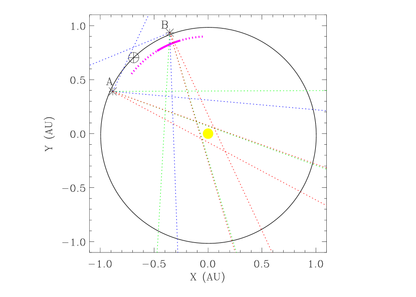
Figure 1: The locations of Earth, STEREO-A, STEREO-B, and the Sun (at the origin) on 2008 February 4 in heliocentric aries ecliptic coordinates. The red, green, and blue dotted lines indicate the fields of view of the COR2, HI1, and HI2 telescopes on board STEREO-A and B. The purple arc is an estimated location for the Feb. 4 CME’s leading edge as it approaches 1 AU, where the part of the arc represented as a solid line is the part of the CME that we detect in SECCHI images from STEREO-A images, and the dotted line indicates the parts of the CME front that we do not see (see §3.2).

The two STEREO spacecraft were launched on 2006 October 26, one into an orbit slightly inside that of Earth (STEREO-A), which means that it moves ahead of the Earth in its orbit, and one into an orbit slightly outside that of Earth (STEREO-B), which means that it trails behind the Earth. Since launch the separation of the A and B spacecraft has been gradually growing. Figure 1 shows their locations on 2008 February 4, which is the initiation date of the CME of interest here. At this point STEREO A and B had achieved a separation angle of $45.3^{\circ}$ relative to the Sun.

The two STEREO spacecraft contain identical sets of instruments. The imaging instruments are contained in a package called the Sun-Earth Connection Coronal and Heliospheric Investigation (SECCHI), which will be described in more detail below. There are two in situ instruments on board, the Plasma and Suprathermal Ion Composition (PLASTIC) instrument (Galvin et al., 2008), and the In-situ Measurements of Particles and CMEs Transients (IMPACT) package (Acuña et al., 2008; Luhmann et al., 2008). The former studies the properties of ions in the bulk solar wind, and the latter studies electrons, energetic particles, and magnetic fields in the IPM. Finally, there is a radio wave detector aboard each spacecraft called STEREO/WAVES, or SWAVES (Bougeret et al., 2008), but SWAVES did not see any activity relevant to our particular CME.

Most of the data presented in this paper will be from the five telescopes that constitute SECCHI, which are fully described by Howard et al. (2008). Moving from the Sun outwards, these consist firstly of an Extreme Ultraviolet Imager (EUVI), which observes the Sun in several extreme ultraviolet bandpasses. There are then two coronagraphs, COR1 and COR2, which observe the white light corona at elongation angles from the Sun of $0.37^{\circ}-1.07^{\circ}$ and $0.7^{\circ}-4.2^{\circ}$, respectively. These angles correspond to distances in the plane of the sky of $1.4-4.0$ R_⊙ for COR1 and $2.5-15.6$ R_⊙ for COR2. Finally, there are the two Heliospheric Imagers, HI1 and HI2, mentioned in §1, which observe the white light IPM in between the Sun and Earth at elongation angles from the Sun of $3.9^{\circ}-24.1^{\circ}$ and $19^{\circ}-89^{\circ}$, respectively. At these large angles, plane-of-sky distances become very misleading, so we do not quote any here. Figure 1 shows explicitly the overlapping COR2, HI1, and HI2 fields of view for STEREO-A and STEREO-B on 2008 February 4.

3 THE 2008 FEBRUARY 4 CME

3.1 Imaging the Event

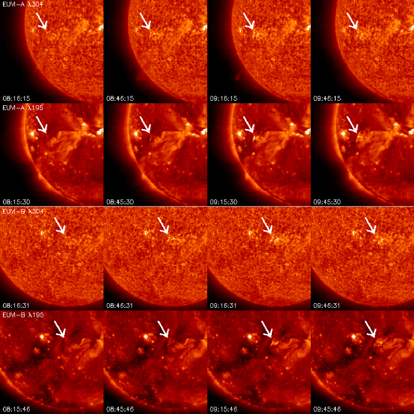
Figure 2: Sequences of EUVI images taken near the beginning of the 2008 Feb. 4 CME. The upper 2 sequences are He II $\lambda$304 and Fe XII $\lambda$195 images from STEREO-A and the bottom 2 sequences are He II and Fe XII images from STEREO-B. The arrows point to a region that flares weakly during the event. The EUVI-A He II $\lambda$304 images also show a prominence eruption off the southeast limb.

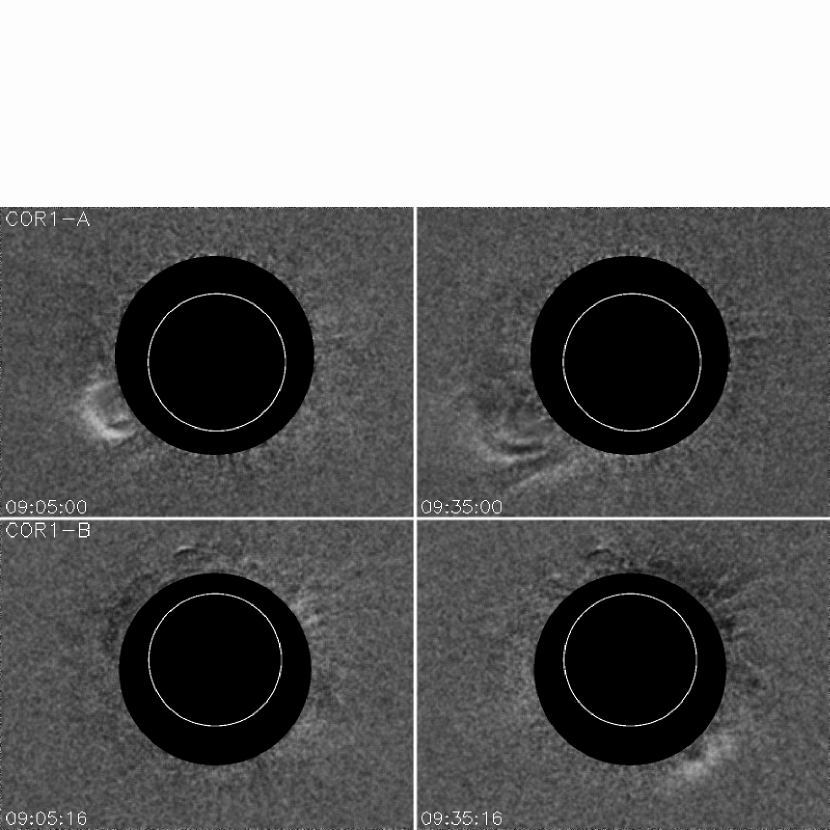
Figure 3: Running-difference COR1 images from STEREO-A (top) and STEREO-B (bottom) showing the 2008 Feb. 4 CME erupting off the southeast limb in COR1-A, but primarily off the southwest limb in COR1-B. The white circle indicates the location of the solar disk.

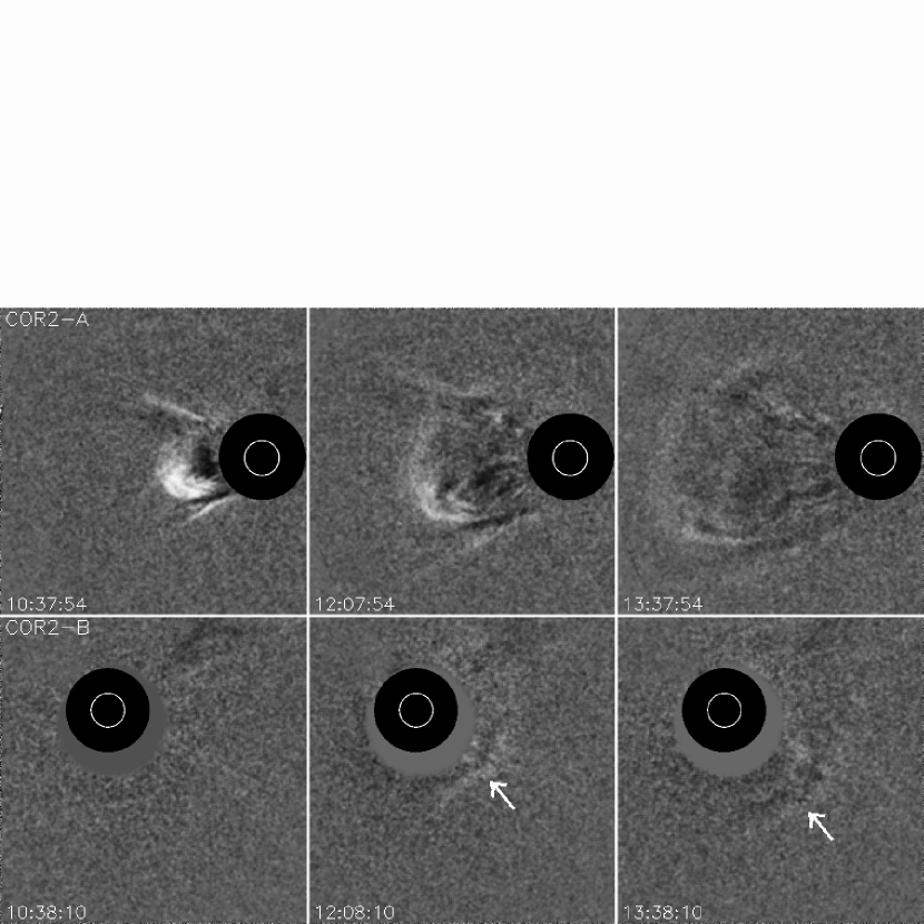
Figure 4: Running-difference COR2 images from STEREO-A (top) and STEREO-B (bottom) showing the 2008 Feb. 4 CME. The CME is clearly seen off the east limb in COR2-A, but it is much fainter and primarily off the southwest limb in COR2-B (arrows). The white circle indicates the location of the solar disk. Beyond the occulter there is some additional masking for COR2-B to hide blooming caused by a slight miscentering of the Sun behind the occulting disk.

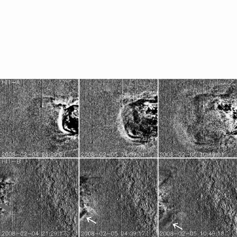
Figure 5: Running-difference HI1 images from STEREO-A (top) and STEREO-B (bottom) showing the 2008 Feb. 4 CME. The Sun is to the right in the HI1-A images and to the left for HI1-B (see Fig. 1). The CME front is obvious in HI1-A, but is only faintly visible in the lower left corner of the last two HI1-B images (arrows).

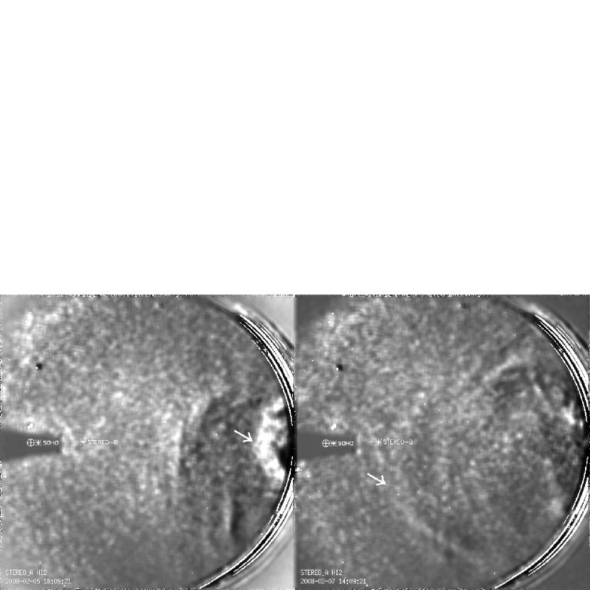
Figure 6: Running-difference HI2 images from STEREO-A showing the 2008 Feb. 4 CME (arrows). The positions of the Earth, SOHO, and STEREO-B are also shown. The first image shows the bright CME front as it enters the field of view on Feb. 5, but the CME front quickly fades and becomes confused with a CIR structure in the background, which is gradually rotating towards the observer. The second image shows the CME front just before it crosses the apparent position of STEREO-B on Feb. 7.

Figures 2–6 provide examples of images of the February 4 event from all five of the SECCHI telescopes. Figure 2 shows sequences of images in two of the four bandpasses monitored by EUVI: the He II $\lambda$304 bandpass and the Fe XII $\lambda$195 bandpass. Note that the actual time cadence is 10 minutes in both of these bandpasses, rather than the 30 minute time separation of the chosen images in Figure 2.

At about 8:16 UT a prominence is observed to be gradually expanding off the southeast limb of the Sun in the EUVI-A $\lambda$304 images. This expansion then accelerates into a full prominence eruption, as a small flare begins at about 8:36 in the He II and Fe XII images some distance northwest of the prominence. The flaring site is indicated by an arrow in Figure 2. This is not a strong flare in EUVI, and there is no GOES X-ray event recorded at all at this time, so the flare is apparently too weak to produce sufficient high temperature plasma to yield a GOES detection.

Figures 3 and 4 show white-light COR1 and COR2 images of a CME that emerges shortly after the EUVI flare begins. As was the case for EUVI, the actual time cadence is three times faster than implied by the selected images: 10 minutes for COR1 and 30 minutes for COR2. The synoptic COR1 and COR2 programs actually involve the acquisition of 3 separate images at three different polarization angles, which we combine into a single total-brightness image for our purposes. [Technically, the COR2 cadence is actually 15 minutes, alternating between the acquisition of full polarization triplets, which we use here, and total brightness images computed from polarization doublets combined onboard, which we do not use (Howard et al., 2008).] The coronagraph images are all displayed in running-difference mode in Figures 3 and 4, where the previous image is subtracted from each image. This is a simple way to subtract static coronal structures and emphasize the dynamic CME material.

From the perspective of STEREO-A the CME is first seen by COR1-A off the southeast limb, as expected based on the location of the flare and prominence eruption. However, the strong southern component to the CME motion seen in the COR1-A images in Figure 3 disappears by the time the CME leaves the COR2-A field of view. In the final COR2-A image in Figure 4 the CME is roughly symmetric about the ecliptic plane, in contrast to its COR1-A appearance. Cremades & Bothmer (2004) have noted that near solar minimum, CMEs appear to be deflected towards the ecliptic plane, presumably due to the presence of high speed wind and open magnetic field lines emanating from polar coronal holes. The February 4 CME may be another example of this.

The CME’s appearance is radically different from the point of view of STEREO-B, illustrating the value of the multiple-viewpoint STEREO mission concept. The EUVI-B flare is only $10^{\circ}$ from disk center, so the expectation is that any CME observed by STEREO-B will be a halo event directed at the spacecraft. However, the COR1-B and COR2-B images show only a rather faint front expanding slowly in a southwesterly direction, though the COR2-B movies do provide hints of expansion at other position angles, meaning that this might qualify as a partial halo CME. It is possible that if the CME was much brighter it might have been a full halo event. It is impressive how much fainter the event is from STEREO-B than from STEREO-A, possibly due to the CME subtending a larger solid angle from STEREO-B’s perspective, with some of the CME blocked by the occulter. The visibility of a CME as a function of viewing angle can also be affected by various Thomson scattering effects (Andrews, 2002; Vourlidas & Howard, 2006).

Both COR1-A and COR1-B (see Fig. 3) show a CME directed more to the south than would be expected based on the flare site (see Fig. 2), and COR1-B shows more of a westward direction than would be expected considering how close to disk center the flare is from the point of view of STEREO-B. We speculate that perhaps the coronal hole just east of the flare site (see EUVI-B Fe XII $\lambda$195 images in Fig. 2) plays a role in deflecting the CME into the more southwesterly trajectory seen by STEREO-B. Thus, this CME seems to show evidence for two separate deflections from coronal holes: the initial deflection to the southwest from the low latitude hole adjacent to the flare site, and the more gradual deflection back towards the ecliptic plane seen in COR2-A (see Fig. 4).

Figures 5 and 6 show HI1 and HI2 images of the CME as it propagates through the IPM to 1 AU. As was the case for COR1 and COR2, the HI1 and HI2 data are displayed in running difference mode. The time cadence of HI1 and HI2 data acquisition are 40 minutes and 2 hours, respectively.

The large fields of view of the HI telescopes and the increasing faintness of CME fronts as they move further from the Sun make subtraction of the stellar background a very important issue. For HI1 we first subtract an average image computed from about 2 days worth of data encompassing the Feb. 4 event. This removes the static F-corona emission, which eliminates the large brightness gradient in the raw HI1 images. We then use a simple median filtering technique to subtract the stars before the running difference subtraction of the previous image is made. Artifacts from some of the brightest stars are still discernible in Figure 5, including vertical streaks due to exposure during the readout of the detector. Median filtering does not work well for the diffuse background produced by the Milky Way, so the Milky Way’s presence on the right side of the HI1-B images is still readily apparent. A somewhat more complicated procedure is used for HI2, which involves the shifting of the previous image before it is subtracted to make the running-difference sequence, in an effort to better eliminate the stellar background. This method should be effective for both the diffuse Milky Way and stellar point source background, but median filtering is also used to further improve the stellar subtraction. The HI2 image processing procedure is described in more detail by Sheeley et al. (2008b).

The bright CME front is readily apparent in the HI1-A images, but in HI1-B the CME can only be clearly discerned in the lower left corner of the last two images in Figure 5. This is consistent with expectations from the appearance of the CME in the COR2 data. The situation becomes more complicated in the HI2 field of view (FOV). Figure 6 shows two HI2-A images, and also shows the positions of Earth, SOHO, and STEREO-B in the FOV. Earth and SOHO are behind a trapezoidal occulter, which is used to prevent the image from being contaminated by a very overexposed image of Earth. The first image shows that the CME front is initially a bright, semicircular front, consistent with its appearance in HI1-A. But it quickly fades, becoming much harder to follow. There are other fronts in the FOV (see Fig. 6) associated with a corotating interaction region (CIR), which confuses things further. The CME front appears to overtake the CIR material and the second image in Figure 6 shows the CME as it approaches the position of STEREO-B. At this point the front is much more well defined in the southern hemisphere than in the north.

Given the potential confusion between our CME front and the CIR material, it is worthwhile to briefly review what CIRs are and how they are perceived by STEREO. Sheeley et al. (2008a, b) have already described CIR fronts seen by HI2 in some detail, which have been the most prominent structures regularly seen by HI2 in STEREO’s first year of operation. The CIRs are basically standing waves of compressed solar wind, where high speed wind coming from low latitude coronal holes is running into low speed wind. The CIRs stretch outwards from the Sun in a spiral shape due to the solar rotation, and have a substantial density enhancement that HI2-A sees as a gradually outward propagating front (or series of fronts) as the CIR rotates into view. The HI2-B imager does not see the approach of the CIR in the distance like HI2-A does because HI2-B is looking at the west side of the Sun rotating away from the spacecraft instead of the east side rotating towards it, where HI2-A is looking (see Fig. 1). Instead, when the CIR reaches STEREO-B, HI2-B seen a very broad front pass very rapidly through the foreground of the FOV as the CIR passes over and past the spacecraft.

Since our CME front appears to overtake a CIR in the HI2-A images, it is tempting to look for evidence of interaction between the two. However, we believe that the leading edge of the CME is actually always ahead of the CIR. The appearance of “overtaking” is due to a projection effect, where the faster moving CME is in the foreground while the apparently slower CIR material seen in Figure 6 is in the background. Support for this interpretation is provided by Figure 2. The EUVI-B Fe XII $\lambda$195 images show the coronal hole that is the probable source of the high speed wind responsible for the CIR. The coronal hole is just east of the flare region that represents the CME initiation site, so with respect to the Sun’s westward rotation the CME leads the high speed wind that yields the CIR. This is the same coronal hole that we suppose to have deflected the CME into a more southwesterly direction, but the leading edge of the CME is always ahead of the CIR. Nevertheless, it is quite possible that the sides and trailing parts of the CME may be interacting with the CIR structure. Trying to find clear evidence for this in the HI2 data ideally requires guidance from models of CME/CIR interaction. Such an investigation is clearly a worthwhile endeavor, but it is outside the scope of our purely empirical analysis here.

Returning to the CME, just as HI2-B does not see CIRs until they engulf STEREO-B, HI2-B does not perceive the February 4 CME until it is practically on top of the spacecraft (as seen from STEREO-A). As the CME approaches and passes over STEREO-B, HI2-B sees a very broad, faint front pass rapidly through the foreground of the FOV, similar in appearance to the CIR fronts described above. Though the rapid front is apparent in HI2-B movies, its faintness combined with its very broad and diffuse nature makes it practically impossible to discern in still images, so we have not attempted to show it in any HI2-B images here.

3.2 In Situ Observations

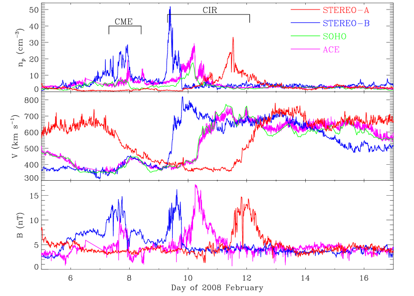
Figure 7: Proton density, solar wind velocity, and magnetic field strength are plotted versus time using data from the PLASTIC and IMPACT instruments on STEREO A and B. Also included are data from ACE and the CELIAS instrument on SOHO, both residing at Earth’s L1 Lagrangian point. The 2008 Feb. 4 CME is observed by STEREO-B on Feb. 7, and much more weakly by ACE and SOHO/CELIAS. It is not seen at all by STEREO-A. A CIR is observed a couple days after the CME by STEREO-B, at a later time by SOHO/CELIAS and ACE, and later still by STEREO-A as the structure rotates past the various spacecraft.

Figures 2-6 demonstrate STEREO’s ability to track a CME continuously from its origin all the way out to 1 AU using the SECCHI telescopes, even for a modest event like the February 4 CME. Figure 7 demonstrates STEREO’s ability to study the properties of the CME when it gets to 1 AU. The upper two panels of Figure 7 show the solar wind proton density and velocity sampled by the PLASTIC experiments on both STEREO spacecraft from February 5-17, and the bottom panel shows the magnetic field strength observed by IMPACT. For comparison, we have also added measurements made at Earth’s L1 Lagrangian point by ACE and SOHO/CELIAS. Including both ACE and SOHO/CELIAS data provides us with two independent measurements at L1. (The CELIAS instrument does not provide magnetic field measurements, though.) The CME is detected by STEREO-B, and more weakly by ACE and SOHO, but it is not detected at all by STEREO-A.

Given that the CME’s initiation site is near Sun-center as seen by STEREO-B (see Fig. 2), it is not surprising that the CME eventually hits that spacecraft. STEREO-B sees a density and magnetic field increase on February 7 at the same time that HI2-A sees the CME front reach STEREO-B, so there is good reason to believe that this is the expected ICME corresponding to the February 4 CME. However, the particle and field response are not characteristic of a typical ICME or magnetic cloud (see, e.g., Jian et al., 2006), and it is difficult to tell exactly where the ICME begins and ends. The wind velocity increases from an ambient slow solar wind speed of about 360 km s^-1 to the CME’s propagation speed of 450 km s^-1, but the velocity increase trails the density and magnetic field increase by at least 12 hours. Perhaps much of the field and density excess associated with the CME may be slow solar wind that has been overtaken and piled up in front of the original CME front, but we cannot rule out the possibility that the CME may be mixed up with some other magnetic structure, confusing the ICME signature in Figure 7. Another possibility is that the central axis of the CME passed to the south of the spacecraft, leading to a more muddled magnetic field signature.

The ICME is also detected by ACE and CELIAS. The velocity profiles seen at L1 are practically identical to that seen by PLASTIC-B. The density profiles seen by ACE and CELIAS are somewhat discrepant. The ACE data show a weak, narrow density spike at the time of maximum density at STEREO-B, while the CELIAS data only show a broad, weak density enhancement. In any case, the density enhancement at L1 is weaker than at STEREO-B. The magnetic field enhancement seen by ACE is also weaker than at STEREO-B, and shorter in duration. Thus, STEREO-B receives a more direct hit from the CME than ACE and SOHO, which are $23.6^{\circ}$ away from STEREO-B (see Fig. 1). This is once again consistent with the CME’s direction inferred from the SECCHI images. At an angle from STEREO-B of $45.3^{\circ}$, the PLASTIC and IMPACT instruments on STEREO-A do not see the CME at all, providing a hard upper limit for the angular extent of the CME in the ecliptic plane.

It is worthwhile to compare and contrast how HI2 and the in situ instruments perceive the CME. The CME front seen by HI2-A (see Fig. 6) appears to reach the location of STEREO-B at about 18:00 UT on February 7. This corresponds roughly to the time when the densest part of the CME is passing by STEREO-B (see Fig. 7). However, both the density and magnetic field data indicate that less dense parts of the CME front reach STEREO-B much earlier. This demonstrates that much of the CME structure is unseen by HI2-A. The HI2-A front displayed in Figure 6 is only the densest part of the CME. For ACE and SOHO there is an even greater disconnect between the HI2-A CME front and the in situ observations of it. Movies of the fading CME front allow it to just barely be tracked out to the position of ACE and SOHO, which it reaches at about 6:00 UT on February 8, well after the weak density enhancement seen by these instruments is over. This means that HI2-A does not see the part of the CME that hits the spacecraft at L1, only seeing the denser parts of the structure that are farther away than L1, in the general direction of STEREO-B.

This leads to the schematic picture of the CME geometry shown in Figure 1. Based on the velocity curves in Figure 7, there is essentially no velocity difference along the CME front, and no time delay between the CME arrival at STEREO-B and L1, so the CME front is presumably roughly spherical as it approaches 1 AU, as shown in Figure 1. However, we have argued above that HI2-A only sees the densest part of the CME, which hits STEREO-B, and HI2-A does not see the foreground part that hits L1 and Earth at all. The dotted purple line in Figure 1 crudely estimates the full extent of the CME, which we know hits STEREO-B, ACE, and SOHO but not STEREO-A, while the shorter solid line arc is an estimate of the part of the CME that HI2-A actually sees. It is difficult to know how far the CME extends to the right of STEREO-B in Figure 1. There is little if any emission apparent to the east of the Sun in COR2-B movies (see Fig. 4), which is why we have not extended the CME arc very far to the right of STEREO-B in Figure 1. Thus, the final picture is that of a CME that has a total angular extent of no more than $60^{\circ}$, with the visible part of the CME constituting less than half of that total.

Besides showing the CME signatures observed by PLASTIC, IMPACT, ACE, and CELIAS, Figure 7 also shows these instruments’ observations of the CIR that follows, the presence of which is also apparent in the HI2-A images in Figure 6, as noted in §3.1. All these spacecraft see a strong density and magnetic field enhancement, which is accompanied by a big jump in wind velocity as the spacecraft passes from the slow solar wind in front of the CIR to the high speed wind that trails it. Such signatures are typical of CIRs seen by in situ instruments (e.g., Sheeley et al., 2008a, b). There is a significant time delay between when the CIR hits STEREO-B, then ACE and SOHO, and finally STEREO-A. This time delay illustrates the rotating nature of the CIR structure. It is curious that the time delay is significantly longer between ACE/SOHO and STEREO-A than it is between STEREO-B and ACE/SOHO despite the angular separation being about the same (see Fig. 1). It is also interesting that the density, velocity, and magnetic field profiles seen by the three spacecraft are rather different. Though outside the scope of this paper, a more in-depth analysis of this and other STEREO-observed CIRs is certainly worthwhile, especially given the substantial number of these structures observed by STEREO in the past year.

3.3 Kinematic Analysis

Possibly the simplest scientifically useful measurements one can make from a sequence of CME images are measurements of the velocity of the CME as a function of time. However, even these seemingly simple measurements are complicated by uncertainties in how to translate apparent 2-dimensional motion into actual 3-dimensional velocity. We now do a kinematic analysis of the February 4 CME, and in the process we show how comprehensive STEREO observations can improve confidence in such an analysis.

In order to measure the velocity and acceleration of a CME’s leading edge, positional measurements must first be made from the SECCHI images. What we actually measure is not distance but an elongation angle, $\epsilon$, from Sun center. Many previous authors have discussed methods of inferring distance from Sun-center, $r$, from $\epsilon$ (Kahler & Webb, 2007; Howard et al., 2007, 2008; Sheeley et al., 2008b). One approach, sometimes referred to as the “Point-P Method,” assumes the CME leading edge is an intrinsically very broad, uniform, spherical front centered on the Sun, in which case (Howard et al., 2007)

$$r=d\sin\epsilon.$$ (1)

Here $d$ is the distance of the observer to the Sun, which is close to 1 AU for the STEREO spacecraft, but not exactly (see Fig. 1).

Another approach, which Kahler & Webb (2007) call the “Fixed-$\phi$ Method,” assumes that the CME is a relatively narrow, compact structure traveling on a fixed, radial trajectory at an angle, $\phi$, relative to the observer’s line of sight to the Sun, in which case

$$r=\frac{d\sin\epsilon}{\sin(\epsilon+\phi)}.$$ (2)

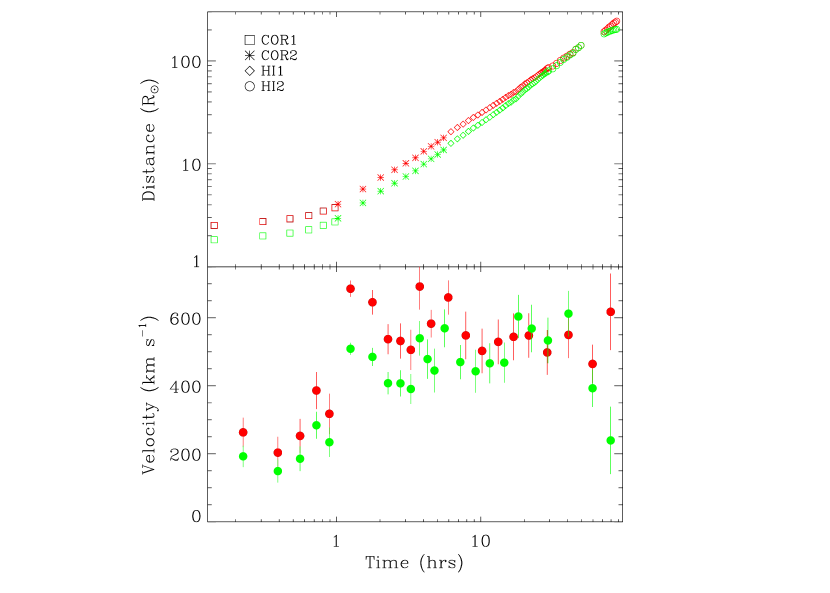
Figure 8: The top panel shows two different versions of the distance-vs.-time plot for the leading edge of the Feb. 4 CME, computed using two different methods to get from measured elongation angle to physical distance from Sun-center. The green measurements assume the “Point-P” method (equation 1), and the red data points assume the “Fixed-$\phi$” method (equation 2). The symbols indicate which SECCHI imager on STEREO-A is responsible for the measurement. The bottom panel shows velocities computed from the distance measurements.

[Note that this is a more compact version of equation (A2) in Kahler & Webb (2007).] In the top panel of Figure 8, we show plots of $r$ versus time, as seen from STEREO-A, using both equations (1) and (2). In the latter case we have assumed the CME trajectory is radial from the flare site, meaning $\phi=46^{\circ}$. There is a time gap in the HI2 measurements, corresponding to when the CME front is too confused with CIR material to make a reliable measurement.

The bottom panel of Figure 8 shows velocities computed from the distance measurements in the top panel. Velocities computed strictly from adjacent distance data points often lead to velocities with huge error bars, which vary wildly in time in a very misleading fashion. For this reason, as we compute velocities from the distances point-by-point we actually skip distance points until the uncertainty in the computed velocity ends up under some assumed threshold value (70 km s^-1 in this case), similar to what we have done in past analyses of SOHO data (Wood et al., 1999). The velocity uncertainties are computed assuming the following estimates for the uncertainties in the distance measurements: 1% fractional errors for the COR1 and COR2 distances, and 2% and 3% uncertainties for HI1 and HI2, respectively.

There are significant differences in the distance and velocity measurements that result from the use of equations (1) and (2). In order to explore the reasons behind the distance differences, first note that a point in an image represents a direction vector in 3D space. If this vector has a closest approach to the Sun at some point P, the geometry assumed by the Point-P method always assumes that this point P represents the real 3D location of the apparent leading edge seen by the observer. Thus, distances estimated using equation (1) by definition represent a lower bound on the actual distance (Howard et al., 2007), explaining why the Point-P data points are always at or below the Fixed-$\phi$ data points in Figure 8.

The two methods lead to different inferences about the CME’s kinematic behavior. The Fixed-$\phi$ method implies an acceleration up to a maximum velocity of about 700 km s^-1 in the COR2 FOV, followed by a gradual deceleration through HI1 and into HI2. In contrast, the Point-P method suggests that the CME accelerates to about 500 km s^-1 in the COR2 FOV and then continues to accelerate more gradually through HI1 and into HI2, before decelerating precipitously in HI2. However, this last precipitous deceleration is clearly an erroneous artifact of the Point-P geometry, which assumes that the CME has a very broad angular extent, encompassing all potentially observed position angles relative to the Sun, and implicitly assuming that the CME engulfs the observer when it reaches 1 AU. That is why equation (1) does not even allow the possibility of measuring $r$ greater than 1 AU. However, we know that the Feb. 4 CME does not hit the observer (i.e., STEREO-A).

We have argued near the end of §3.2 that the Feb. 4 CME does not have a very large angular extent, and that the extent of the observed part of the CME is even more limited (see Fig. 1). Thus, the Fixed-$\phi$ geometry is a much better approximation for this particular event. It is important to note that this conclusion will not be the case for broader, brighter CMEs, where the Point P approach might work better. The Fixed-$\phi$ method does have the disadvantage that it requires a reasonably accurate knowledge of $\phi$, though the known flare location provides a good estimate. And as the CME travels outwards, there will still be some degree of uncertainty introduced by the likelihood that the observed leading edge is not precisely following precisely the same part of the CME structure at all times.

The effects of these uncertainties can be explored by comparing the CME velocities measured in the HI2-A FOV with the in situ velocity observed by PLASTIC-B. If the uncertainties are low, the SECCHI image-derived velocities should agree well with the PLASTIC-B velocity. The Fixed-$\phi$ velocities measured in the HI2 FOV in Figure 8 (at times of $t\gtrsim 30$ hr) average around 530 km s^-1, somewhat higher than the 450 km s^-1 velocity seen by PLASTIC-B (see Fig. 7). This is presumably indicative of the aforementioned systematic uncertainties. Figure 9 illustrates how the discrepancy can be addressed by lowering the assumed CME trajectory angle, $\phi$. Figure 9 plots $r$ versus $\phi$ for many values of $\phi$, computed using equation (2). The curves steepen in the HI2 FOV ($\epsilon=19^{\circ}-89^{\circ}$) as $\phi$ increases, meaning that velocities inferred from these distances will also increase. Thus, lowering $\phi$ below the $\phi=46^{\circ}$ value assumed in Figure 8 will lower the inferred HI2 velocities.

In order to determine which $\phi$ value works best, we perform a somewhat more sophisticated kinematic analysis than that in Figure 8. Compared to the point-by-point analysis used in Figure 8, a cleaner and smoother velocity profile can be derived from the data if the distance measurements are fitted with some functional form, which in essence assumes that the timescale of velocity variation is long compared to the time difference between adjacent distance measurements. Polynomial or spline fits are examples of such functional forms that can used for these purposes. However, we ultimately decide on a different approach, relying on a very simple physical model of the CME’s motion. This model assumes an initial acceleration for the CME, $a_{1}$, which persists until a time, $t_{1}$, followed by a second acceleration (or deceleration), $a_{2}$, lasting until time $t_{2}$, followed finally by constant velocity. This model also has two additional free parameters: a starting height, and a time shift of the model distance-time profile to match the data. The two-phase model bears some resemblance to the “main” and “residual” acceleration phases of a CME argued for by Zhang & Dere (2006). But to us the appeal of this simple model is that not only are its parameters physical ones of interest, it also seems to fit the data as well or better than more complex functional forms, despite having only six free parameters.

Figure 10 shows our best fit to the data using this model. The top panel shows the leading edge distances computed assuming $\phi=38^{\circ}$, which turns out to be the value that leads to the observed PLASTIC-B velocity of 450 km s^-1 in the HI2-A FOV. The solid line shows our best fit to the data, determined using a chi-squared minimization routine, where we have assumed the same fractional errors in the distance measurements as we did in Figure 8 (see above). With these assumed uncertainties, the best fit ends up with a reduced chi-squared of $\chi_{\nu}^{2}=1.33$. This agrees well with the $\chi_{\nu}^{2}\approx 1$ value expected for a good fit (Bevington & Robinson, 1992), which implies that the error bars assumed for our measurements are neither unrealistically small nor unreasonably large.

The bottom two panels of the figure show the velocity and acceleration profiles implied by this fit. The velocity at 1 AU (214 $R_{\odot}$) in the HI2-A FOV ends up at 450 km s^-1 as promised. It should be emphasized that in forcing the HI2-A velocity to be consistent with the PLASTIC-B measurement, we are implicitly assuming that the part of the CME front being observed by HI2-A has the same velocity as the part of the CME front that hits STEREO-B. Essentially, this amounts to assuming that the CME front is roughly spherical and centered on the Sun at 1 AU, as pictured in Figure 1 and argued for in §3.2. The excellent agreement between the CME velocity seen by PLASTIC-B and that seen at L1 by ACE and SOHO/CELIAS also implies that this assumption is a very good one for this event. But this may not be the case for all events, so comparing HI2-A and PLASTIC-B velocities may not always be appropriate.

The $\phi=38^{\circ}$ value assumed in Figure 10 is $8^{\circ}$ less than the $\phi=46^{\circ}$ value that radial outflow from the observed flare site would suggest. This result could indicate that the CME’s overall center-of-mass trajectory is truly at least $8^{\circ}$ closer to the STEREO-A direction than the flare site would predict. (More if there is a component of deflection perpendicular to the ecliptic plane.) In §3.1 we noted that the COR1-B and COR2-B images imply a deflection of the CME into a more southwesterly trajectory than suggested by the flare site, possibly due to the adjacent coronal hole. The western component of this deflection would indeed predict a CME trajectory less than $\phi=46^{\circ}$ angle suggested by the flare. Thus, interpreting the $8^{\circ}$ shift as due to this deflection is quite plausible.

However, this interpretation comes with two major caveats. One is that the part of the CME seen as the leading edge by HI2-A is not necessarily representative of either the geometric center of the CME, or its center-of-mass. Measurements from a location different from that of STEREO-A could in principle see a different part of the CME front as being the leading edge, thereby leading to a different trajectory measurement. The second caveat is the aforementioned issue of the observed leading edge not necessarily faithfully following the same part of the CME front at all times, which could yield velocity measurement errors and therefore an erroneous $\phi$ measurement.

Figure 10 represents our best kinematic model of the February 4 CME, which can be described as follows. The model suggests that the CME’s leading edge has an initial acceleration of $a_{1}=159$ m s^-2 for its first $t_{1}=1.1$ hours, reaching a maximum velocity of 689 km s^-1 shortly after entering the COR2 FOV. Until $t_{2}=33$ hours the CME then gradually decelerates at a rate of $a_{2}=-2.1$ m s^-2 during its journey through the COR2 and HI1 fields of view, eventually reaching its final coast velocity of 451 km s^-1 shortly after reaching the HI2 FOV, this velocity being consistent with the PLASTIC-B measurement.

Interaction with the ambient solar wind is presumably responsible for the $a_{2}$ deceleration inferred between 0.024 and 0.47 AU, as the PLASTIC-B data make it clear that the CME is traveling through slower solar wind plasma. Note that the Point-P measurements in Figure 8 are not only inconsistent with this $a_{2}$ IPM deceleration, but they would actually imply an acceleration of the CME at that time. This emphasizes the importance of the issue of how to compute distances from elongation angles. Even basic qualitative aspects of a CMEs IPM motion, such as whether it accelerates or decelerates, depend sensitively on this issue. Given that the CME is plowing through slower solar wind material, an IPM deceleration seems far more plausible than an acceleration. This is yet another argument that the Fixed-$\phi$ geometry is better for this particular event than the Point-P geometry.

3.4 Implications for Space Weather Prediction

An event like the February 4 CME is perfect for assessing the degree to which the unique viewpoint of the STEREO spacecraft can yield better estimates of arrival times for Earth-directed CMEs. The February 4 CME is directed at STEREO-B, so STEREO-B’s in situ instruments tell us exactly when the CME reaches 1 AU, but the STEREO-B images of the event close to the Sun provide very poor velocity estimates by themselves because of the lack of knowledge of the CME’s precise trajectory. For full halo CMEs, Schwenn et al. (2005) provide a prescription to determine the true expansion velocity from its lateral expansion (see also Schwenn, 2006). But the uncertainties remain large, and in any case this prescription is not helpful for our February 4 event, which is barely perceived as a partial halo, let alone a full halo. Therefore, it is STEREO-A that by far provides the best assessment of the CME’s kinematic behavior thanks to its location away from the CME’s path. And it is STEREO-A that is therefore in a much better position to predict ahead of time when the event should reach STEREO-B.

To better quantify this, we imagine a situation where only STEREO-B data is available. The CME has just taken place and the CME has been observed by COR1-B and COR2-B as shown in Figures 3 and 4. We can then ask the question, what would our estimated CME velocity be from the STEREO-B data alone and what would be the predicted arrival time at 1 AU? The apparent plane-of-sky velocity of the CME in the COR2-B images is about 240 km s^-1 (assuming $\phi=90^{\circ}$). The total travel time to Earth at this speed is about 174 hours, leading to a predicted arrival time of roughly Februrary 11, 15:00 UT. This is 4 days after the actual arrival time on February 7, so this prediction is obviously very poor!

If the EUVI-B flare location is used to provide an estimated trajectory of $\phi=10^{\circ}$, the velocity estimated from the COR2-B data increases dramatically to about 1000 km s^-1. In this case the 1 AU travel time decreases to only 42 hours, corresponding to a predicted arrival time of February 6, 3:00 UT. This is well over a day before the actual arrival time. For events directed at the observing spacecraft, CME velocity measurements are particularly sensitive to uncertainties in the exact trajectory angle. There is also the problem that the observed leading edge motion in the COR2-B images may have more to do with the lateral expansion of the CME rather than the motion outwards from the Sun.

If a similar thought experiment is done for the STEREO-A data, the COR2-A images alone and an assumption of the $\phi=46^{\circ}$ trajectory suggested by the EUVI-A flare site lead to a CME velocity in COR2-A of about 590 km s^-1. This corresponds to a 1 AU travel time of about 71 hours, leading to a predicted arrival time at 1 AU of February 7, 8:00 UT. This is only a few hours after the arrival of the CME suggested by the IMPACT-B magnetic field data (see Fig. 7), though it is about 13 hours before the peak density seen by PLASTIC-B, which is what the CME front observed by the SECCHI imagers actually corresponds to (see §3.3). Improving the arrival time prediction of the peak CME density would require taking into account the deceleration of the CME during its travel through the IPM (see Fig. 10).

It is clear that STEREO-A’s perspective provides a dramatic improvement in our ability to predict when the February 4 CME reaches STEREO-B. An analysis of multiple events like this one would allow this improvement to be better quantified. In the spirit of previous analyses such as Gopalswamy et al. (2001), perhaps an analysis of multiple events such as this one would also provide empirical guidance in how to predict the deceleration during IPM travel (or perhaps acceleration in some cases), which is clearly necessary to achieve arrival time estimates that are good to within a few hours. The ability of SECCHI to provide continuous tracking information on CMEs could in principle allow time-of-arrival estimates to be continously improved during a CME’s journey to 1 AU.

4 SUMMARY

We have presented STEREO observations of a CME that occurred in the depths of the 2008 solar minimum, when there were not many of these events taking place. The February 4 CME is not a particularly dramatic event, but it has an advantageous trajectory. It is directed at STEREO-B, so that it eventually hits that spacecraft and is detected by its in situ instruments. A different part of the CME hits the ACE and SOHO spacecraft at Earth’s L1 Lagrangian point. The CME’s trajectory is far enough away from the STEREO-A direction that STEREO-A images can provide an accurate assessment of the CME’s kinematic behavior, which is not possible from STEREO-B’s location. This event illustrates just how much the appearance of a CME can differ between the two STEREO spacecraft, which at the time had an angular separation relative to the Sun of $45.3^{\circ}$, a separation that continues to increase with time by about $44^{\circ}$ per year.

Despite the relative faintness of the event, the SECCHI imagers are still able to track it continuously all the way from the Sun to 1 AU, which provides hope that as the Sun moves towards solar maximum, STEREO will be able to provide similarly comprehensive observations of many more such CMEs. The kinematic analysis presented here is the first based on such a comprehensive STEREO data set, involving both SECCHI images and in situ data, but hopefully many others will follow. We have used two different methods of computing CME leading edge distances from measured elongation angles: 1. The Point-P method, which assumes the CME is a broad, uniform, spherical front; and 2. The Fixed-$\phi$ method, which assumes a narrow, compact CME structure traveling radially from the Sun. Our analysis illustrates just how sensitive conclusions about the kinematic behavior of a CME are to the method used. The first method suggests continued acceleration in the IPM, while the second implies a deceleration. Fortunately, the comprehensive nature of observations of the February 4 CME has provided us with an abundance of evidence that the observable part of this CME has a very limited angular extent. Therefore, the Fixed-$\phi$ method is clearly best in this case, leading to our best kinematic model for the CME in Figure 10. But we do not expect the Fixed-$\phi$ method to necessarily be the best option for all STEREO-observed CMEs.

Finally, the geometry of the event allows us to use the two spacecrafts’ observations to quantify just how much more accurately the CME’s arrival time at 1 AU can be predicted using images taken away from the CME’s path (from STEREO-A in this case), compared to images taken from directly within it (from STEREO-B in this case). The STEREO-A prediction proves to be dramatically better than STEREO-B’s. Thus, STEREO could in principle be able to improve space weather forecasting for Earth-directed events in the coming years.

Figure 9: A plot of inferred distance from Sun-center ($r$) as a function of measured elongation angle $\epsilon$, for seven values of the CME trajectory angle $\phi$, using equation (2). The $\phi=46^{\circ}$ curve is emphasized since that is the trajectory angle suggested by the flare location (see Fig. 2).

Figure 10: The top panel shows the distance from Sun-center of the leading edge of the 2008 Feb. 4 CME as a function of time, assuming the CME trajectory angle is $\phi=38^{\circ}$ from the line of sight. The $t=0$ time is 8:36 UT, roughly when the flare associated with this CME begins. The symbols indicate which SECCHI imager on STEREO-A is responsible for the measurement. The data points are fitted with a simple kinematic model assuming an initial acceleration phase, a second deceleration phase, and then a constant velocity phase. The best fit is shown as a solid line in the top panel. The bottom two panels show the velocity and acceleration profiles suggested by this fit.

References

- Acuña et al. (2008) Acuña, M. H., Curtis, D., Scheifele, J. L., Russell, C. T., Schroeder, P., Szabo, A., & Luhmann, J. G. 2008, Space Sci. Rev., 136, 203
- Andrews (2002) Andrews, M. D. 2002, Sol. Phys., 208, 317
- Bevington & Robinson (1992) Bevington, P. R., & Robinson, D. K. 1992, Data Reduction and Error Analysis for the Physical Sciences (New York: McGraw-Hill)
- Bougeret et al. (2008) Bougeret, J. L., et al. 2008, Space Sci. Rev., 136, 487
- Cremades & Bothmer (2004) Cremades, H., & Bothmer, V. 2004, A&A, 422, 307
- Eyles et al. (2003) Eyles, C. J., et al. 2003, Sol. Phys., 217, 319
- Galvin et al. (2008) Galvin, A. B., et al. 2008, Space Sci. Rev., 136, 437
- Gopalswamy et al. (2001) Gopalswamy, N., Lara, A., Yashiro, S., Kaiser, M. L., & Howard, R. A. 2001, J. Geophys. Res., 106, 29207
- Harrison et al. (2008) Harrison, R. A., et al. 2008, Sol. Phys., 247, 171
- Howard et al. (2008) Howard, R. A, et al. 2008, Space Sci. Rev., 136, 67
- Howard et al. (2007) Howard, T. A., Fry, C. D., Johnston, J. C., & Webb, D. F. 2007, ApJ, 667, 610
- Howard et al. (2008) Howard, T. A., Nandy, D., & Koepke, A. C. 2008, J. Geophys. Res., 113, A01104
- Jackson et al. (2004) Jackson, B. V., et al. 2004, Sol. Phys., 225, 177
- Jian et al. (2006) Jian, L., Russell, C. T., Luhmann, J. G., & Skoug, R. M. 2006, Sol. Phys., 239, 393
- Kahler & Webb (2007) Kahler, S. W., & Webb, D. F. 2007, J. Geophys. Res., 112, A09103
- Luhmann et al. (2008) Luhmann, J. G., et al. 2008, Space Sci. Rev., 136, 117
- Schwenn (2006) Schwenn, R. 2006, Living Rev. Solar Phys. 3, 2, URL: http://www.livingreviews.org/lrsp-2006-2
- Schwenn et al. (2005) Schwenn, R., dal Lago, A., Huttunen, E., & Gonzalez, W. D., 2005, Ann. Geophys., 23, 1033
- Sheeley et al. (2008a) Sheeley, N. R., Jr., et al. 2008a, ApJ, 674, L109
- Sheeley et al. (2008b) Sheeley, N. R., Jr., et al. 2008b, ApJ, 675, 853
- Vourlidas & Howard (2006) Vourlidas, A., & Howard, R. A. 2006, ApJ, 642, 1216
- Webb et al. (2006) Webb, D. F., et al. 2006, J. Geophys. Res., 111, A12101
- Wood et al. (1999) Wood, B. E., Karovska, M., Chen, J., Brueckner, G. E., Cook, J. W., & Howard, R. A. 1999, ApJ, 512, 484
- Zhang & Dere (2006) Zhang, J., & Dere, K. P. 2006, ApJ, 649, 1100