Differential Rotation and Meridional Circulation in Global Models of Solar Convection

Abstract

In the outer envelope of the Sun and in other stars, differential rotation and meridional circulation are maintained via the redistribution of momentum and energy by convective motions. In order to properly capture such processes in a numerical model, the correct spherical geometry is essential. In this paper I review recent insights into the maintenance of mean flows in the solar interior obtained from high-resolution simulations of solar convection in rotating spherical shells. The Coriolis force induces a Reynolds stress which transports angular momentum equatorward and also yields latitudinal variations in the convective heat flux. Meridional circulations induced by baroclinicity and rotational shear further redistribute angular momentum and alter the mean stratification. This gives rise to a complex nonlinear interplay between turbulent convection, differential rotation, meridional circulation, and the mean specific entropy profile. I will describe how this drama plays out in our simulations as well as in solar and stellar convection zones.

1 Introduction

Axisymmetric flows are a key component of virtually all solar dynamo models. Differential rotation is thought to be the principal mechanism by which toroidal field is continually regenerated from poloidal field. In the language of mean-field dynamo theory, this is known as the $\Omega$-effect and the Sun may be classified as an $\alpha$-$\Omega$ dynamo (e.g. Ossendrijver 2003; Charbonneau 2005). Furthermore, many recent dynamo models, known as flux-transport models, suggest that global axisymmetric circulations in the meridional plane (latitude-radius) may account for the observed migration of active regions toward the equator during the course of the solar activity cycle and may thus determine the cycle period (e.g. Wang et al. 1991; Choudhuri et al. 1995; Dikpati & Charbonneau 1999; Dikpati & Gilman 2006).

The internal rotation profile of the Sun is well established from helioseismology (Thompson et al. 2003) and as we have seen at this meeting, there is ample evidence for the presence of differential rotation in other stars (see other papers in these proceedings as well as previous work by Barnes et al. 2005 and Reiners 2006). In the solar convection zone the angular velocity decreases monotonically by about 30% from equator to pole with nearly radial contours at mid latitudes. Regions of stronger radial shear exist near the top and bottom of the convective zone, the latter known as the solar tachocline.

The meridional circulation is more challenging to detect but photospheric measurements and local helioseismic inversions have revealed a systematic but variable poleward flow of 15-20 m s^-1 in the upper solar convection zone (e.g. Hathaway 1996; Haber et al. 2002; Gonzáles-Hernández et al. 2006).

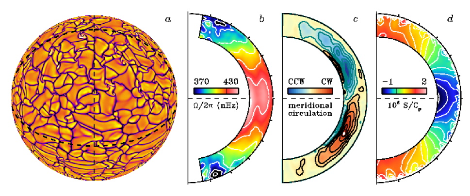
Figure 1: Flow features in a simulation of solar convection. ($a$) Radial velocity near the top of the computational domain ($r=0.98R$) with yellow tones denoting upflow and blue/black tones denoting downflow. This orthographic projection is tilted 35^∘ toward the line of sight so the north pole is visible. ($b$) Differential rotation, ($c$) meridional circulation, and ($d$) specific entropy perturbations averaged over longitude and time (132 days). The meridional circulation is represented as streamlines of the mass flux and the entropy is normalized by the specific heat at constant pressure $C_{P}=3.5\times 10^{8}$ erg g^-1 K^-1 (after Miesch et al. 2007).

Differential rotation and meridional circulation in the solar envelope and in other stars are maintained by convection. The highly turbulent nature of solar and stellar convection makes numerical modeling a difficult challenge but contininuing advances in supercomputing technology have enabled increasingly realistic 3D simulations. In this paper I’ll review what our most recent convection simulations reveal about the nature of mean flows in the solar envelope and how they are maintained.

2 Turbulent Solar Convection

High-resolution simulations of solar convection exhibit intricate flow structures and persistent mean flows as illustrated in Figure 1. The simulation shown was carried out using the ASH (Anelastic Spherical Harmonic) computer code described by Clune et al. (1999) and Brun, Miesch & Toomre (2004). The ASH code solves the three-dimensional equations of hydrodynamics (or magneto-hydrodynamics) in a rotating spherical-shell geometry under the anelastic approximation. The simulation shown in Figure 1 extends from the base of the convective envelope at $0.71R$, where $R$ is the solar radius, to $0.98R$, within about 14 Mm of the photosphere. Beyond $0.98R$, granulation and supergranulation occur in the Sun which cannot be resolved in a global model (yet) and which involve physical processes neglected in ASH such as ionization and radiative transfer. Solar values are used for the luminosity and rotation rate and the background stratification is based on a solar structure model. For further details on this simulation see Miesch et al. (2007).

Near the top of the computational domain there is an interconnected network of downflow lanes which appears similar to solar granulation but occupies a much larger scale (Fig. 1$a$). These giant cells are about 100 Mm across on average, compared to 30 Mm for supergranulation and 1 Mm for granulation. At high and mid latitudes, the downflow lanes exhibit intense cyclonic vorticity (counter-clockwise in the northern hemisphere, clockwise in the southern), which is evident in animations of the convective patterns.

The correlation time for the downflow network is 2-3 days, depending on latitude, but closer scrutiny reveals longer-lived structures (Miesch et al. 2007). At low latitudes, persistent downflow lanes occur which are oriented in a north-south direction and which persist for weeks to months. These are traveling convection modes which propagate prograde faster than the local rotation rate. Although the downflow network fragments deeper down, the north-south downflow lanes extend through most of the convection zone and play an important role in the maintenence of mean flows (§3).

The differential rotation achieved in this simulation is shown in Figure 1$b$. It is roughly solar-like, with a monotonic decrease in the angular velocity from equator to pole and relatively little variation with radius across the convection zone. However, the angular velocity contrast between the equator and $\pm 60^{\circ}$ is only about 50 nHz, compared to 90 nHz in the Sun. Other ASH simulations have achieved better agreement with helioseismic inversions, including a stronger angular velocity contrast and nearly radial angular velocity contours at mid latitudes (Miesch et al. 2006).

Figure 1$c$ shows the meridional circulation which is dominated by a single cell in each hemisphere, with poleward flow in the upper convection zone (amplitude 15-20 m s^-1) and equatorward flow in the lower convection zone (amplitude 5-10 m s^-1). This is roughly consistent with flux transport solar dynamo models and helioseismic determinations of the meridional circulation in the upper convection zone of the Sun (§1).

Although the circulation pattern in Figure 1$c$ is predominatly single-celled in each hemisphere, narrow counter-cells occur near the top and bottom boundaries. In light of our idealized boundary conditions (stress-free, impenetrable, imposed specific entropy profile on the bottom and constant heat flux on the top), the presence of these counter-cells should be interpreted with caution. ASH simulations which incorporate convective penetration into an underlying radiative zone generally exhibit equatorward meridional circulation throughout the overshoot region (Miesch et al. 2000). Furthermore, angular momentum transport by supergranulation may induce a systematic poleward circulation in the surface layers via a process known as gyroscopic pumping (see eq. (1) below).

Figure 1$a$, $b$, and $c$ illustrate convection, differential rotation, and meridional circulation. Before proceeding to §3, there is one more player in this drama to be introduced. Figure 1$d$ shows the mean specific entropy perturbation $\left<S\right>$ relative to the spherically symmetric background stratification, averaged over longitude and time. The $\left<S\right>$ profile exhibits prominent warm poles associated with thermal wind balance (§3). The corresponding temperature variation is $\sim$ 8K (Miesch et al. 2007, Fig. 6) which is more than five orders of magnitude smaller than the background temperature of 2.2 million K at the base of the convection zone. However, whereas the specific entropy perturbation increases monotonically with latitude throughout the convection zone, the temperature perturbation near the top of the shell typically peaks at the poles and the equator, with a minimum at mid-latitudes (Brun & Toomre 2002; Miesch et al. 2006).

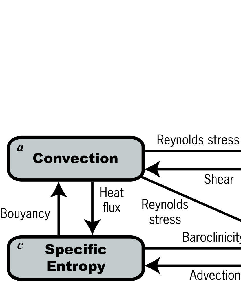
Figure 2: Schematic diagram illustrating the complex nonlinear coupling between ($a$) convection, ($b$) differential rotation, ($c$) the mean specific entropy profile $\left<S\right>$, and ($d$) the meridional circulation (see text).

3 Maintenance of Mean Flows

In order to understand how mean flows are maintained in our convection simulations and, by extension, in the Sun and in other stars, two equations are particularly enlightening. The first is derived from the zonal (longitudinal) component of the momentum equation, averaged over longitude and time:

$${\bf\nabla\cdot}\left(\overline{\rho}\left<{\bf v}_{m}\right>{\cal L}\right)=-{\bf\nabla\cdot}\left(\overline{\rho}r\sin\theta\left<v_{\phi}^{\prime}{\bf v}_{m}^{\prime}\right>\right)$$ (1)

where ${\cal L}$ is the specific angular momentum

$${\cal L}=r\sin\theta\left(\Omega r\sin\theta+\left<v_{\phi}\right>\right)~{}~{}~{}.$$

Equation (1) is expressed in a rotating spherical polar coordinate system with radius $r$, colatitude $\theta$, and longitude $\phi$ and corresponding velocity components $v_{r}$, $v_{\theta}$, and $v_{\phi}$. The meridional velocity component is defined as ${\bf v}_{m}=v_{r}{\bf\hat{r}}+v_{\theta}{\bf\hat{\theta}}$ where ${\bf\hat{r}}$ and ${\bf\hat{\theta}}$ are unit vectors in the $r$ and $\theta$ directions. Brackets $<>$ denote averages over longitude and time, and primes indicate fluctuating variables for which the mean has been subtracted out, e.g. $v_{\phi}^{\prime}=v_{\phi}-\left<v_{\phi}\right>$. The rotation rate of the coordinate system is $\Omega$ and $\overline{\rho}$ is the (spherically symmetric) background density stratification.

The second equation of particular importance is derived from the zonal component of the vorticity equation which is the curl of the momentum equation:

$${\bf\Omega\cdot\nabla}\left<v_{\phi}\right>=\frac{g}{2rC_{P}}\frac{\partial\left<S\right>}{\partial\theta}$$ (2)

where $\left<S\right>$ is the mean specific entropy perturbation as in Fig. 1$d$, $g$ is the gravitational acceleration, and $C_{P}$ is the specific heat per unit mass at constant pressure.

When deriving equations (1) and (2) we have assumed that the system in question (whether it be a simulation or a star) is in a statistically steady state. Furthermore, we have neglected viscous dissipation which is significant in some simulations but insignificant in stellar interiors where the Reynolds number (the ratio of inertial to viscous forces) is of order 10¹² or more. We have also neglected the Lorentz force which generally has a dissipative effect in the convection zone, suppressing rotational shear (Brun et al. 2004). In the tachocline, Lorentz forces associated with strong, localized toroidal field structures may divert or induce meridional and zonal flows.

Equation (2) involves several additional assumptions, most notably that the Coriolis force operating on the differential rotation is large relative to the Reynolds stress. In other words, we have assumed that the Rossby number $Ro=\omega/2\Omega$ is much less than unity, where $\omega$ is the fluid vorticity in the rotating frame. The Rossby number is not specified in ASH simulations; rather, it is computed a posteriori from the simulated flow field. Results generally indicate that the small $Ro$ assumption implied by equation (2) is valid in the lower convection zone but breaks down near the surface where the amplitude of $\omega$ peaks.

When deriving equation (2) we have also assumed an ideal gas equation of state and that the background stratification is hydrostatic and adiabatic to lowest order. Both of these assumptions are well justified in the bulk of the solar convection zone but break down for $r>0.98R$.

Subject to these reasonable assumptions, equation (1) states that the advection of angular momentum by the meridional circulation $\left<{\bf v}_{m}\right>$ must balance the angular momentum transport due to the Reynolds stress $\left<v_{\phi}^{\prime}{\bf v}_{m}^{\prime}\right>$. The Reynolds stress arises from correlations in the convective velocity components induced by the Coriolis force. Of particular relevance are the north-south oriented downflow lanes mentioned in §2; as horizontal flows near the top of the convection zone converge into these downflow lanes, eastward flows are diverted equatorward by the Coriolis force and westward flows are diverted poleward. This produces an equatorward angular momentum transport which is mainly responsible for the prograde equatorial rotation seen in Figure 1$b$.

Equation (2) states that gradients in the mean zonal velocity (as well as the mean angular velocity) parallel to the rotation axis are proportional to the latitudinal entropy gradient. This is the solar analogue of thermal wind balance which has been studied for decades within the context of geophysics (e.g. Pedlosky 1987). In the absence of latitudinal entropy gradients, equation (2) implies cylindrical rotation profiles in which angular velocity (and zonal velocity) contours are parallel to the rotation axis. This is a manifestation of the well-known Taylor-Proudman theorem.

Insight into how the dynamical balances expressed by equations (1) and (2) are achieved can be gained by considering Figure 2. Convection redistributes momentum and can establish differential rotation (DR) and meridional circulation (MC) through the Reynolds stress ($a\rightarrow b$, $a\rightarrow d$). It can also alter the mean entropy profile by means of the convective heat flux which includes contributions from enthalpy flux as well as kinetic energy flux ($a\rightarrow c$). Differential rotation can provide a negative feedback by shearing out convection cells ($b\rightarrow a$). Meanwhile, modications of the specific entropy profile alter the buoyancy driving of the convective motions ($c\rightarrow a$). The meridional circulation can in principle feed back directly on the convection as well ($d\rightarrow a$) but in practice this is negligible because the convective kinetic energy generally exceeds that contained in the MC by about two orders of magnitude.

Differential rotation can induce meridional circulations
through the Coriolis force ($b\rightarrow d$) while entropy variations can induce circulations through baroclinicity ($c\rightarrow d$), in particular the $\partial\left<S\right>/\partial\theta$ term on the right-hand-side of equation (2). Advection of angular momentum and entropy by the meridional circulation can in turn alter the $\left<v_{\phi}\right>$ and the $\left<S\right>$ profiles ($d\rightarrow b$, $d\rightarrow c$).

Equation (1) involves panels $a$, $b$, and $d$ of Figure 2, such that angular momentum transport by the convective Reynolds stress ($a\rightarrow b$) balances that by the meridional circulation ($d\rightarrow b$). It is this balance that largely determines the meridional circulation pattern. As the Reynolds stress establishes a differential rotation, the meridional circulation adjusts such that equation (1) is satisfied. In previous, more laminar simulations of convection, angular momentum transport by viscous diffusion upset the balance expressed by equation (1) and circulation patterns were qualitatively different from that in Figure 1$c$, multi-celled in latitude and radius (Miesch et al. 2000, 2006; Brun & Tooomre 2002).

This simplified picture is complicated by the nonlinear feedback mechanisms illustrated in Figure 2 and the additional constraint provided by thermal wind balance, equation (2). Equation (2) only explicitly involves the differential rotation and specific entropy profile ($b$, $c$), but convection and meridional circulation ($a$, $d$) both play an essential role. In order to demonstrate this, we consider now two illustrative scenarios by which thermal wind balance may be achieved. We’ll refer to these as mechanical and thermal forcing (Miesch et al. 2006). Both cases begin with convection ($a$) but they each circle the diagram in Figure 2 in an opposite sense, clockwise and counter-clockwise respectively.

In the mechanical forcing scenario, the convective Reynolds stress establishes a differential rotation ($a\rightarrow b$) which induces a meridional circulation via the Coriolis force ($b\rightarrow c$). The advection of entropy by these circulations then alters the background stratification $\left<S\right>$ ($c\rightarrow d$). In the subadiabatic portion of the tachocline, this would tend to establish warm poles and the Coriolis-induced circulations would cease when thermal wind balance, equation (2), is achieved (Rempel 2005; Miesch et al 2006). However, in the convection zone the sense of the induced circulation is such that the resulting latitudinal entropy gradient would be equatorward rather than poleward (cool poles). Thermal wind balance would be achieved eventually, but the rotation profile would not be solar-like.

Now consider thermal forcing in which a latitude-dependent convective heat flux establishes warm poles ($a\rightarrow c$) which in turn induce a meridional circulation through baroclinicity ($c\rightarrow d$). Redistribution of angular momentum by this baroclinic circulation then establishes a differential rotation ($d\rightarrow b$). This will ‘work’ in the sense that the induced DR will evolve until equation (2) is satisfied. However, in the absence of the Reynolds stress, the meridional circulation would tend to conserve angular momentum, accelerating the poles relative to the equator. This follows from equation (1); if the right-hand-side is zero and ${\bf\nabla\cdot}\left(\overline{\rho}\left<{\bf v}_{m}\right>\right)=0$ as required by the anelastic approximation, then $\left<{\bf v}_{m}\right>{\bf\cdot\nabla}{\cal L}=0$, so ${\cal L}$ would be constant along circulation streamlines. A solar-like differential rotation profile can only be achieved if the Reynolds stress also contributes, transporting angular momentum toward the equator ($a\rightarrow b$).

Thus, the convective Reynolds stress is needed to produce a prograde equatorial rotation relative to higher latitudes as in the Sun while baroclinicity is needed to break the Taylor-Proudman preference for cylindrical rotation profiles. Such baroclinicity arises from a latitude-dependent convective heat flux but thermal coupling to the tachocline may also play an important role (Rempel 2005; Miesch et al. 2006). Much has been learned but much remains to be done and convection simulations will continue to provide valuable insight into how differential rotation and meridional circulation are established and maintained in the Sun and in stars across the HR diagram.

The work reported here is done in close collaboration with our “ASH mob” of Allan Sacha Brun, Juri Toomre, Marc DeRosa, Matthew Browning, Benjamin Brown, Nicholas Featherstone, Kyle Augustson, and Nicholas Nelson. Funding was provided by NASA through grant NNG05G124G of the Heliophysics Theory Program. The simulations were carried out with NSF PACI support of PSC, SDSC, and NCSA and NASA support through Project Columbia.

References

- [1] Barnes, J.R, Collier-Cameron, A., Donati, J.-F., James, D.J. Marsden, S.C., Petit, P.: 2005, MNRAS, 357, L1-L5
- [2] Brun, A.S., Miesch, M.S., Toomre, J.: 2004, ApJ, 614, 1073
- [3] Brun, A.S., Toomre, J.: 2002, ApJ, 570, 865
- [4] Dikpati, M., Charbonneau, P.: 1999, ApJ, 518, 508
- [5] Dikpati, M., Gilman, P.A.: 2006, ApJ, 649, 498
- [6] Charbonneau, P.: 2005, Living Rev. Solar Phys., 2, 2, http://www.livingreviews.org/lrsp-2005-2
- [7] Choudhuri, A.R., Schüssler, M., Dikpati, M.: 1995, A&A, 303, L29
- [8] Clune, T.C., Elliott, J.R., Miesch, M.S., Toomre, J., Glatzmaier, G.A.: 1999, Parallel Computing, 25, 361
- [9] Haber, D.A., Hindman, B.W, Toomre, J., Bogart, R.S., Larsen, R.M, Hill, F.: 2002, ApJ, 570, 855
- [10] Hathaway, D.H.: 1996, ApJ, 460, 1027
- [11] González-Hernández, I., Komm, R., Hill, F., Howe, R., Corbard, T. Haber, D.A.: 2006, ApJ, 638, 576
- [12] Miesch, M.S., Brun, A.S., Toomre, J.: 2006, ApJ 641, 618
- [13] Miesch, M.S, Brun, A.S., DeRosa, M.L., Toomre, J.: 2007, ApJ, submitted
- [14] Miesch, M.S, Elliott, J.R., Toomre, J., Clune, T.C., Glatzmaier, G.A, Gilman, P.A.: 2000, ApJ, 532, 593
- [15] Ossendrijver, M.: 2003, Astron. Astrophys. Rev., 11, 287
- [16] Pedlosky, J.: 1987, Geophysical Fluid Dynamics (Springer-Verlag: New York), second edition
- [17] Reiners, A.: 2006, A&A, 446, 267
- [18] Rempel, M.: 2005, ApJ, 622, 1320
- [19] Thompson, M.J., Christensen-Dalsgaard, J., Miesch, M.S., Toomre, J.: 2003, Ann. Rev. Astron. Astrophys., 41, 599
- [20] Wang, Y.-M., Sheeley Jr, N.R., Nash, A.G.: 1991, ApJ, 383, 431