An explanation for the pseudogap of high-temperature superconductors based on quantum optics

Abstract

We first explain the pseudogap of high-temperature superconductivity based on an approach of quantum optics. After introducing a damping factor for the lifetime $\tau$ of quasiparticles, the superconducting dome is naturally produced, and the pseudogap is the consequence of pairing with damped coherence. We derive a new expression of Ginzburg-Landau free energy density, in which a six-order term due to decoherence damping effect is included. Without invoking any microscopic pairing mechanism, this approach provides a simple universal equation of second-order phase transition, which can be reduced to two well-known empirical scaling equations: the superconducting dome Presland-Tallon equation, and the normal-state pseudogap crossover temperature $T^{*}$ line.

Besides the unveiled microscopic mechanism, the remarkable mysteries of high-temperature superconductivity (HTSC) are the superconducting dome, the HTSC transition temperature $T_{c}$ as a function of doping, and pseudogap in phase diagram Millis ; Emery1 ; Norman1 . It is believed that, a correct explanation for the superconducting dome and pseudogap is strongly related to the origin of HTSC. However, there is no convincing explanation with detailed analytical expressions for the superconducting dome and pseudogap region. Its origin and physical interpretation are fundamental questions in HTSC  Millis ; Emery1 ; Norman1 . There are two most popular physical models on HTSC: Resonating-valence-bond (RVB) picture Anderson ; Lee and quantum critical scenario Tallon ; Norman2 . The former origins from the idea of spin singlet scenario Nagaosa and that the pseudogap is a precursor to the superconducting state, which is pairing without long-range phase coherence Emery2 . The latter origins form the idea that another state of matter, pseudogap phase, competes with superconducting gap for the same Fermi surface.

In this paper,we first apply quantum optics approach to explain HTSC, and show that the experimental results of superconducting dome together with pseudogap can be described by a universal equation of second-order phase transition. The superconducting dome and normal-state pseudogap crossover temperature in HTSC are attributed to the finite lifetime of cooper pairs due to decoherence damping, which results in localized cooper pairs with limited phase coherence. We also present a modified general Ginzburg-Landau free energy density (GLFED), which includes a sixth-order term due to this decoherence damping effect. This phenomenological two-state model does not invoke any microscopic pairing mechanism, but can provide a simple universal equation, which can be reduced to two well-known empirical scaling equations: the superconducting dome Presland-Tallon equation Presland , and the normal-state pseudogap crossover temperature $T^{*}$ line Huefner .

Before applying quantum optics approach, we should list some commonly accepted facts we ensure for HTSC: (1) Superconductivity is due to the formation of Cooper pairs with long-range order Tsuei ; Harlingen , which are spin singlet and have $d_{x^{2}-y^{2}}$ orbital symmetry. (2) Photoemission experiments reveal sharp spectral peaks in the excitation spectrm Damascelli , indicating the presence of quasiparticle states. (3) The essential structure is the CuO₂ planes, and the formation of Cooper pairs takes place independently within different multiplayers Dagotto . (4) The electron-phonon interaction is not the principal mechanism of the formation of Cooper pairs Anderson2 . (5) The Cooper pairs are formed from the time-reversed states (called as non-pairing breaking) Leggett .

First we show the BCS Hamiltonian can be expressed in quantum optics approach. The Hamiltonian of the whole system can be expressed as $H=\sum_{i=0}^{4}H_{i}$, where

$$H_{0}=\sum_{\mathbf{p},\sigma,\mathrm{i}}\left(\varepsilon_{\mathbf{p}}-\mu\right)c^{+}_{\mathbf{p},\sigma,\mathrm{i}}c_{\mathbf{p},\sigma,\mathrm{i}}+\sum_{\mathbf{q}}\hbar\omega_{\mathbf{q}}a^{+}_{\mathbf{q}}a_{\mathbf{q}},$$ (1)

is the Hamiltonian of the free system, the Hamiltonian of the interaction between quasiparticles and intermediate bosons is

$$H_{1}=\sum^{\prime}_{\mathbf{p},\mathbf{p}^{\prime},\sigma,\mathrm{i}}M_{\mathbf{p}^{\prime},\mathbf{p}}\left(c^{+}_{\mathbf{p}^{\prime},\sigma,\mathrm{i}}c_{\mathbf{p},\sigma,\mathrm{i}}a_{\mathbf{p}^{\prime}-\mathbf{p}}+H.c\right),$$ (2)

the Hamiltonian of the repulsive interaction between quasiparticle and quasiparticle is

$$H_{2}=\sum^{\prime}_{\mathbf{p},\mathbf{p}^{\prime},\mathrm{i}}V_{\mathbf{p}^{\prime},\mathbf{p}}c^{+}_{\mathbf{p}^{\prime},\uparrow,\mathrm{i}}c^{+}_{-\mathbf{p}^{\prime},\downarrow,\mathrm{i}}c_{-\mathbf{p},\downarrow,\mathrm{i}}c_{\mathbf{p},\uparrow,\mathrm{i}},$$ (3)

and the coupling Hamiltonian between neighboring CuO₂ layers is

$$H_{3}=\sum^{\prime}_{\mathbf{p},\sigma,\mathrm{i}}U\left(c^{+}_{\mathbf{p},\sigma,\mathrm{i}}c_{\mathbf{p},\sigma,\mathrm{i}+1}+c^{+}_{\mathbf{p},\sigma,\mathrm{i}+1}c_{\mathbf{p},\sigma,\mathrm{i}}\right),$$ (4)

and the random Hamiltonian $H_{4}=\sum^{\prime}_{\mathbf{p},\sigma,\mathrm{i}}h^{R}_{\mathbf{p},\sigma,\mathrm{i}}$. $H_{4}$ includes all the random interaction, such as the in-elastic interaction, the random potential caused by doping, and so on. This Hamiltonian could introduce a damping rate of quasiparticles. Here, $\sum^{\prime}_{\mathbf{p},\mathbf{p}^{\prime},\mathrm{i}}$ denotes the sum of quasiparticles that participate in Cooper pairing. $c^{+}_{\mathbf{p},\sigma,\mathrm{i}}$ creates a Fermi-type quasiparticle with momentum state $\mathbf{p}$=($p_{x}$, $p_{y}$), spin $\sigma$ in the $i$th CuO₂ layer. In the low-temperature superconductors, the Cooper pair formed by two electrons is caused by the electron-phonon interaction. It is not true in HTSC as the facts we list above. However, there must be the intermediate bosons being changed among the quasiparticles in order to induce the attractive potential between two quasiparticles. Here we define $a_{\mathbf{q}}$ as the annihilation operator of the intermediate boson with momentum $\mathbf{q}$=($q_{x}$, $q_{y}$). $M_{\mathbf{p}^{\prime},\mathbf{p}}$ is the quasiparticle-boson interaction strength, $V_{\mathbf{p}^{\prime},\mathbf{p}}$ is the quasiparticle-quasiparticle interaction strength and $U$ is the coupling strength between two neighboring layers. $H_{1}$ is the energy of the quasiparticle-quasiparticle repulsive interaction, while $H_{2}$ is the energy of quasiparticle-boson interaction, which could cause Cooper pairing. Here, we ignore the effect of $H_{3}$. If $|H_{2}|>|H_{1}|$, the repulsive interaction will suppress Cooper pairing, for which no superconductivity occurs. However, if $|H_{2}|<|H_{1}|$, many Cooper pairs could be formed, which will leads superconductivity.

In conventional BCS theory, the Hamiltonian of the electron-phonon interaction $H_{1}$ is included in the electron-electron interaction $H_{2}$ resulting an effective attractive potential. However, in HTSC, since there is no consensus on the dispersion of quasiparticle and the $d$-type Fermi surface, it is difficult to follow the conventional BCS approach to investigate HTSC. In this case, we include the $H_{2}$ in $H_{1}$, and the system Hamiltonian is given by $H=H_{0}+V+H_{3}+H_{4}$, where $V=\sum^{\prime}_{\mathbf{p},\mathbf{p}^{\prime},\sigma,\mathrm{i}}h_{\mathbf{p},\mathbf{p}^{\prime},\sigma,\mathrm{i}}$ is the effective quasiparticle-boson interaction, with

$$h_{\mathbf{p},\mathbf{p}^{\prime},\sigma,\mathrm{i}}=M_{\mathbf{p}^{\prime},\mathbf{p}}\left(c^{+}_{\mathbf{p}^{\prime},\sigma,\mathrm{i}}c_{\mathbf{p},\sigma,\mathrm{i}}A_{\mathbf{p}^{\prime}-\mathbf{p},\bar{\sigma}}+H.c\right),$$ (5)

and the effective boson operator $A_{\mathbf{p}^{\prime}-\mathbf{p},\bar{\sigma}}$ is

$$A_{\mathbf{p}^{\prime}-\mathbf{p},\bar{\sigma}}=a_{\mathbf{p}^{\prime}-\mathbf{p}}+\frac{1}{4}\frac{V_{\mathbf{p}^{\prime},\mathbf{p}}}{M_{\mathbf{p}^{\prime},\mathbf{p}}}c^{+}_{-\mathbf{p}^{\prime},\bar{\sigma},\mathrm{i}}c_{-\mathbf{p},\bar{\sigma},\mathrm{i}},$$ (6)

where $\bar{\sigma}$ denotes the opposite $\sigma$. Since the most important physics is included in $H_{0}+V+H_{4}$ and the use of $H_{3}$ is only to ensure the long-range order (there is no long-range order in the two-dimensional system), we only consider the interaction of the two-dimensional system, firstly.

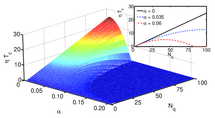
Figure 1: The temperature $\eta T_{c}$ as a function of parameter $\alpha$ and density of quasiparticles $N_{q}$ with zero longitudinal damping $\beta=0$ and $\Delta T=0$. For zero $\alpha$, temperature $T$ is proportional to the density of quasiparticles $N_{q}$. However, in the non-zero $\alpha$ case, the dependence of temperature on $N_{q}$ is arc shape, and dome shape for larger $\alpha$, as shown in the inserted firgure.

The interaction Hamiltonian $V$ is composed by many two-state systems, in which $h_{\mathbf{p},\mathbf{p}^{\prime},\sigma,\mathrm{i}}$ denotes that the two states of quasiparticle, $|e\rangle=|\mathbf{p}^{\prime},\sigma,\mathrm{i}\rangle$ and $|g\rangle=|\mathbf{p},\sigma,\mathrm{i}\rangle$ are coupled by a boson with moment $\mathbf{q}=\mathbf{p}^{\prime}-\mathbf{p}$. The number of intermediate bosons with momentum $\mathbf{q}$ is $\left\langle A^{+}_{\mathbf{p}^{\prime}-\mathbf{p},\bar{\sigma}}A_{\mathbf{p}^{\prime}-\mathbf{p},\bar{\sigma}}\right\rangle$. Here we should emphasize that since $V_{\mathbf{p}^{\prime},\mathbf{p}}>0$ is the repulsive potential and quasiparticle-boson interaction leads an attractive potential, we have

$$\left\langle A^{+}_{\mathbf{p}^{\prime}-\mathbf{p},\bar{\sigma}}A_{\mathbf{p}^{\prime}-\mathbf{p},\bar{\sigma}}\right\rangle<\left\langle a^{+}_{\mathbf{p}^{\prime}-\mathbf{p}}a_{\mathbf{p}^{\prime}-\mathbf{p}}\right\rangle.$$ (7)

which denotes that there is a bias for the Cooper pairing. That is to say only the number of bosons larger than a certain value can Cooper pairing occurs. It will be seen below. $h_{\mathbf{p},\mathbf{p}^{\prime},\sigma,\mathrm{i}}+h^{R}_{\mathbf{p},\sigma,\mathrm{i}}+h^{R}_{\mathbf{p}^{\prime},\sigma,\mathrm{i}}$ can be simply expressed as $h_{e,g}=h^{R}+M_{e,g}\left(c^{+}_{e}c_{g}A_{eg}+H.c\right)$. This model has been well investigated in Quantum Optics Scully . In Heisenberg picture, $\langle c^{+}_{e,g}(t)c_{e,g}(t)\rangle$ give the number of quasiparticles in states $|e,g\rangle$ as a function of time, and $\langle c^{+}_{g}(t)c_{e}(t)\rangle$ denotes the coherence between two quasiparticle states. On the other hand, in the conventional BCS theory, the lifetime quasiparticle is infinite (or very long). However, in HTSC, the random Hamiltonian gives a finite lifetime $\tau=\gamma^{-1}$ to quasiparticle since for arbitrary operator $Q(t)$ we have $\frac{d}{dt}Q(t)=\frac{1}{i\hbar}[Q(t),h^{R}]=-\gamma Q(t)$. The damping rate $\gamma$ includes all the decoherent factors that could destroy the coherence of Cooper pairing and could be expressed as a polynome of the density of quasiparticles, which participate in Cooper pairing, $N_{q}$ (defined below), $\gamma=\Sigma_{j}a_{j}(N_{q})^{j}$. Here we only consider the first two terms, thus $\gamma$ can be written as $\gamma=\gamma_{T}+\gamma_{L}$, where the transverse damping rate $\gamma_{T}=\tau^{-1}_{T}$, which may be caused by spin-exchange collision Wittke , is proportional to $N_{q}$, and $\gamma_{L}=\tau^{-1}_{L}$ denotes the longitudinal damping rate, which is unrelated to $N_{q}$, but relate to the superconductivity-transition temperature $T_{c}$.

Considering the statistic, we define the quantum average variables as $\phi_{\alpha\beta}(t)\equiv\langle c^{+}_{\alpha}(t)c_{\beta}(t)\rangle$. In Heisenberg picture, the dynamic equation for operator $Q(t)$ is $i\hbar\frac{d}{dt}Q(t)=[Q(t),h_{\mathbf{p},\mathbf{p}^{\prime},\sigma,\mathrm{i}}+h^{R}_{\mathbf{p},\sigma,\mathrm{i}}+h^{R}_{\mathbf{p}^{\prime},\sigma,\mathrm{i}}]$, and $i\hbar\frac{d}{dt}Q(t)=[Q(t),h_{\mathbf{p},\mathbf{p}^{\prime},\sigma,\mathrm{i}}]-i\hbar\gamma Q(t)$. Thus, the dynamics of simplified system could be expressed as

$$\frac{d}{dt}\phi_{ee} = -\gamma\phi_{ee}+i\Omega\phi_{ge}-i\Omega^{*}\phi_{eg},$$ (8)

$$\frac{d}{dt}\phi_{gg} = -\gamma\phi_{gg}-i\Omega\phi_{ge}+i\Omega^{*}\phi_{eg},$$ (9)

$$\frac{d}{dt}\phi_{eg} = -\gamma\phi_{eg}-i\Omega\left(\phi_{ee}-\phi_{gg}\right),$$ (10)

where $\Omega=\frac{M_{eg}}{\hbar}\sqrt{n_{bos}-n_{nor}}$ is the general Rabi frequency. We have used the fact that $A_{eg}\approx A^{+}_{eg}\approx\sqrt{n_{bos}-n_{nor}}$ since $(n_{bos}-n_{nor})\gg 1$. $n_{bos}$ is the number of bosons with moment $\mathbf{q}=\mathbf{p}^{\prime}-\mathbf{p}$, and $n_{nor}$ is the equivalent boson number caused by the quasiparticle-quasiparticle repulsive potential. Thus, one could see that the number of bosons should be larger than the bias number $n_{nor}$. If there is no damping factor, $\gamma=0$, the perfect Rabi oscillation of between states $|e,g\rangle$ is presented, which is given by $\phi_{eg}(t)=\frac{i}{2}\sin 2|\Omega|t$. However, if $\gamma\neq 0$, $\phi_{eg}(t)$ should be averaged by the lifetime of quasiparticle $\tau$ as $\bar{\phi}_{eg}=\frac{1}{\tau}\int dt\phi_{eg}(t)e^{-t/\tau}$, which leads to an expression of the second-order phase transition Scully

$$\bar{\phi}_{eg}=\frac{i}{2}\frac{|\Omega|^{2}}{|\Omega|^{2}+\tau^{-2}}.$$ (11)

We define that the quasiparticle density of two states are $n_{e}$ and $n_{g}$, and their sum $n_{e}+n_{g}=n_{q}$ is the density of quasiparticles with momentum $\mathbf{p}^{\prime}$ and $\mathbf{p}$. Since $|\bar{\phi}_{eg}|$ denotes the average value of transition probability, which is also equal with $|\bar{\phi}_{ge}|$, $n_{e}|\bar{\phi}_{eg}|$ gives the number of bosons radiated by the upper state $|e\rangle$, and $n_{g}|\bar{\phi}_{ge}|$ gives the number of bosons absorbed by the lower state $|g\rangle$. By summing all momentum parts and spin, we have that $N_{q}=\sum^{\prime}_{\mathbf{p},\mathbf{p}^{\prime},\sigma}n_{q}$ is the total density of quasiparticles that participate in Cooper pairing, $N_{bos}=\sum^{\prime}_{\mathbf{p},\mathbf{p}^{\prime},\sigma}n_{bos}$ denotes the total density of intermediate bosons, and $N_{nor}=\sum^{\prime}_{\mathbf{p},\mathbf{p}^{\prime},\sigma}n_{nor}$ is the effective bosen density caused by the repulsive interaction.

Since the transverse damping rate $\tau^{-1}_{T}$ is proportional to the number of quasiparticles Wittke while $\tau^{-1}_{L}$ does not, thus $\frac{1}{g\tau_{T}}=\alpha N_{q}$ and $\beta=\frac{1}{g\tau_{L}}$, with $g=\frac{|M_{eg}|}{\hbar}$. $\alpha$ is a proportional parameter, and $\beta$ will be zero for zero traverse damping rate. In the equilibrium state, we have $n_{g}=n_{e}=\frac{1}{2}n_{q}$, and $n_{e}|\bar{\phi}_{eg}|=n_{bos}-n_{nor}$. Thus, the relation between temperature $T$ and the density of quasiparticles $N_{q}$ could be expressed by an equation of second-order phase transition,

$$\eta(T-T_{c})=\alpha^{2}N^{2}_{q}-\left(\frac{1}{4}-2\alpha\beta\right)N_{q}+\eta\Delta T.$$ (12)

Here we have used the fact that $N_{nor}-N_{bos}-\beta^{2}=\eta(T-T_{c}-\Delta T)$, where $\eta$ a proportional parameter to make equal dimension on the two sides of equal sign. This relation is based on the well-known Gingzburg-Landau free energy density (GLFED, see below) Scully . $\eta\Delta T$ is a temperature bias. $T_{c}$ is the critical temperature, below which ($T<T_{c}$) the materials are in the superconducting state. As we have said, $N_{bos}$ is the boson number contributing the attractive potential, while $N_{nor}$ is the effective boson number contributing the repulsive potential. Thus, if $N_{bos}<N_{nor}$ ($T>T_{c}$), the repulsive potential will suppress the attractive potential. No superconductivity occurs in this case. However, the attractive potential will suppress the repulsive potential for $N_{bos}>N_{nor}$ ($T<T_{c}$), which will leads superconductivity transition. In this case, we could get the condition for materials being in the superconducting state from Eq.(12):

$$0\leq-\alpha^{2}N^{2}_{q}+\left(\frac{1}{4}-2\alpha\beta\right)N_{q}-\eta\Delta T\leq\eta T_{c},$$ (13)

and the critical condition of the superconductivity transition

$$\eta T_{c}=-\alpha^{2}N^{2}_{q}+\left(\frac{1}{4}-2\alpha\beta\right)N_{q}-\eta\Delta T.$$ (14)

Figure 1 shows the temperature $T_{c}$ as a function of $N_{q}$ for different parameter $\alpha$ with zero longitudinal damping rate $\beta=0$ and $\Delta T=0$. One could see that, for zero transverse damping rate, $\alpha=0$, the density of quasiparticles $N_{q}$ is proportional to the temperature $T_{c}$. However, for the non-zero $\alpha$ case, the dependence between $T_{c}$ and $N_{q}$ is arc shape, and finally, dome shape. It is very like the pseudogap in the diagram of HTSC, in which $T^{\ast}$ is proportional to the doping, and the dependence between $T_{c}$ and doping is a dome shape. The detailed discussion will be shown in below. By the way, Fig.1 coincides with the results of $\mu$SR measurements in Ref. Uemura .

Equation (12) is the steady result for the system. We could treat it as the consequence of the minimum of GLFED $f_{s}$, if we define an order parameter $\psi_{i}$, of which $|\psi_{i}|^{2}$ gives the density of quasiparticles $N_{q}$. In this case GLFED could be expressed as

$$f_{s} = f_{n}+\left(A|\psi_{i}|^{2}+B|\psi_{i}|^{4}+C|\psi_{i}|^{6}\right)$$ (15)

$$+\frac{U}{N}\sum_{i}\left(\psi_{i}\psi^{*}_{i+1}+c.c\right),$$

where $A=\eta\left(-\Delta T-T_{c}+T\right)/2$, $B=\left(\frac{1}{4}-2\alpha\beta\right)/4$ and $C=-\alpha^{2}/6$, and $N$ is the total number of CuO₂ layers. Below we will see that in the superconductive phase, $\Delta T$ is negative, and $\frac{1}{4}\gg 2\alpha\beta$. $f_{n}$ is the free energy density of the normal state. As one could see, unlike the usual GLFED Chakravarty , the sixth-order term of $|\psi|$, which is completely caused by the damping factors of quasiparticles, is included. We think the the coupling interaction between two neighboring layers less contributes to the free energy. $\Delta T$ is a temperature bias. In the special case, $\alpha=0$, which denotes the lifetime of quasiparticle is infinite, Eq.(15) will come back to the usual form of GLFED.

From above GLFED one could discuss the sample face energy and the response of HTSC in external magnetic field. Here we should denote that: Several phenomenal theories Nagaosa ; Sachdev based on the Ginzburg-Landau equations have been established to explain the pseudogap and superconductivity dome of HTSC. However, these theories have two disadvantages: I. One order parameter corresponds to one phase. Thus what one should find is the order parameter corresponding to the superconductivity phase, but not those for fermion pairing and the Bose condensation in RVB picture or the competing order in quantum critical scenario. II. Pseudogap and the $d$-density wave (DDW) have not been confirmed to be a phase. There is no reason to introduce an order parameter to either.

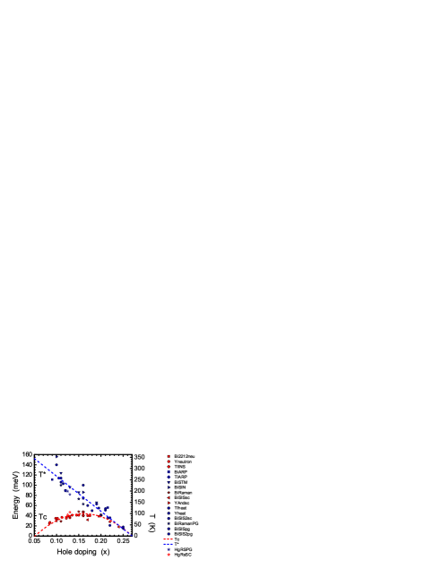
Figure 2: Energy of pseudogap (blue points) and superconducting gap (red points) for a number of HTSCs as measured as a function of hole doping $x$ (obtained from Ref. Huefner ). Lines are the consequences derived from our theory with the parameters $\eta^{-1}=152$ meV, $\alpha=0.27$, $\eta\Delta T=-0.13$, $y=0.24$, $\beta=0.065$ and $\mu=18$. Blue line gives the temperature of pseudogap $T^{\ast}$ ($\alpha=0$), while red line denotes the superconductivity-transition temperature $T_{c}$.

In order to compare with the experiments, we should write Eq.(14) relating to the doping $x$. Since $N_{q}$ must be a function of $x$, it could always be expressed as a polynome of $x$, $N_{q}=\sum_{n}\lambda_{n}x^{n}$. Here we only consider the first two terms, $N_{q}=\nu-\mu x$. Thus, Eq.(14) could be re-expressed as

$$T_{c}=\eta^{-1}\left[-\alpha^{2}\mu^{2}(y-x)^{2}+\left(\frac{1}{4}-2\alpha\beta\right)\mu(y-x)-\eta\Delta T\right],$$ (16)

where $y=\nu/\mu$. As one could see, for the ”localized” measurements, which do not include the transverse damping factor, $\alpha=0$, the temperature is linear proportional to the doping $x$. We believe it corresponds to the temperature $T^{\ast}$ of pseudogap Norman1 . On the other hand, in fact, quasiparticles have finite lifetime, which leads non-zero $\alpha$. The dependence between temperature and doping is arc shape, and dome shape for lager parameter $\alpha$. In this case, Eq. (16) simultaneously involves the well-known two empirical equations Presland ; Huefner : $E_{pg}=E^{\textrm{max}}_{pg}(0.27-x)/0.22$, $E_{sc}=E^{\textrm{max}}_{sc}\left[1-82.6(0.16-x)^{2}\right]$. Figure 2 shows the comparison between our theoretical result and the experimental datum of Ref. Huefner . They perfectly match each other. We think that the experimental techniques Timusk , such as angle-resolved photonmission (ARP) Damascelli and nuclear magnetic resonance (NMR) Warren , only detect the ”localized” character of pairs and do not include the effective transverse damping factor. This predicts $T_{c}$ will increase with small transverse damping factor $\alpha$.

From above discussion, one could see that the function of doping is only to dilute the density of quasiparticles (or Cooper pairs) and consequently to increase the effective lifetime of quasiparticle (long-range coherence). In the low-doped region, the number of quasiparticles is so large that their lifetimes are very short, which leads the short-range order. At the optimal doping, the number of Cooper pairs and their coherence match very well. In the over-doped region, the number of Cooper pairs decrease, which reduces the superconductivity $T_{c}$.

In conculion, we have applied an approach of quantum optics to explain the pseudogap in HTSC. By introducing the effective lifetime of quasiparticle, the superconducting dome is naturally produced. We also derive a new expression of GLFED, which includes the six-order term of order parameter and could simultaneously give the two well-known empirical formulas Presland ; Huefner . The main results of this letter are the modified general GLFED expression Eq. (6) and the universal equation of second-order phase transition Eq. (8). Despite the simplicity of this approach, these general and universal expressions should provide new insights into the origin of HTSC.

This work is supported by MOST of China under Grant No. 2005CB724500.

References

- (1) A. J. Millis, Science 314, 1888 (2006).
- (2) M. R. Norman, D. Pines, and C. Kallin, Adv. Phys. 54, 715 (2005).
- (3) V. J. Emery, S. A. Kivelson and O. Zachar, Phys. Rev. B 56, 6120 (1997).
- (4) P. W. Anderson, Science 235, 1196 (1987).
- (5) P. A. Lee, N. Nagaosa and Xiao-Gang Wen, Rev. Mod. Phys. 78, 17 (2006).
- (6) J. L. Tallon et al., Phys. Stat. Sol. 215, 531 (1999).
- (7) M. R. Norman, and C. Pepin, Rep. Prog. Phys. 66, 1547 (2003).
- (8) N. Nagaosa, and P. A. Lee, Phys. Rev. B 45, 966 (1992).
- (9) V. J. Emery, and S. A. Kivelson, Nature 374, 434 (1995).
- (10) M. R. Presland, J.L.Tallon, R.G.Buckley, R.S.Liu and N.E.Flower, Physica C 176, 95 (1991).
- (11) S. Huefner, M. A. Hossain, A. Damascelli, and G. Sawatzky, Rep. Prog. Phys. 71, 062501 (2008).
- (12) C. C. Tsuei and J. R. Kirtley, Rev. Mod. Phys. 72, 969 (2000).
- (13) Van Harlingen, D. J. Rev. Mod. Phys. 67, 515 (1995).
- (14) A. Damascelli, Z. Hussain and Zhi-Xun Shen, Rev. Mod. Phys. 75, 473 (2003).
- (15) E. Dagotto, Rev. Mod. Phys. 66, 763 (1994).
- (16) P. W. Anderson, Science 288, 480 (2000).
- (17) A. J. Leggett, Quantum Liquids (Oxford Univ. Press, Oxford, 2006).
- (18) Y. J. Uemura, et al., Phys. Rev. Lett. 62, 2317 (1989).
- (19) M. O. Scully and M. S. Zubairy, Quantum Optics (Cambridge Univ. Press, 1997), Chapter 6 and 11.
- (20) J. P. Wittke, R. H. Dicke, Phys. Rev. 103, 620 (1956).
- (21) S. Chakravarty, et al., Nature 428, 53 (2004).
- (22) S. Sachdev, Phys. Rev. B 45, 389 (1992).
- (23) T. Timusk, and B. Statt, Rep. Prog. Phys. 62, 61 (1999).
- (24) W. W. J. Warren, et al., Phys. Rev. Lett. 62, 1193 (1989).
- (25) H. Alloul, T. Ohno, and P. Mendels, Phys. Rev. Lett. 63, 1700. (1989).