Thermo-spin effects in a quantum dot connected to ferromagnetic leads

Abstract

We study a system composed of a quantum dot in contact with ferromagnetic leads, held at different temperatures. Spin analogues to the thermopower and thermoelectric figures of merit are defined and studied as a function of junction parameters. It is shown that in contrast to bulk ferromagnets, the spin thermopower coefficient in a junction can be as large as the Seebeck coefficient, resulting in a large spin figure of merit. In addition, it is demonstrated that the junction can be tuned to supply only spin current but no charge current. We also discuss experimental systems where our predictions can be verified.

Introduction. – Thermoelectricity - the relation between a temperature bias and a voltage bias - is a very old problem of solid-state physics. It has gained renewed interest in recent years Mahan ; Majumdar ; book due to the prospect of utilizing nanostructures to develop high efficiency thermoelectric converters Hochbaum ; Boukai . Theoretical models have been put forward for the thermoelectric transport through quantum point contacts, QPCtheory ; ourwork quantum dots,QDtheory ; Krawiec ; Subroto , molecular junctions MolJuncTHeory and other strongly correlated nanostructures Freericks .

Recently, Uchida et al.Uchida have measured the spin equivalent of the charge Seebeck coefficient, namely the spin Seebeck effect, in which a temperature difference between the edges of a bulk ferromagnetic (FM) slab induces a spin-voltage difference and generates spin current. These authors have suggested using this effect to construct a spin-current source for spintronic devices spintronics . However, the spin-Seebeck coefficient in this experiment was measured to be four orders of magnitude smaller than the charge Seebeck coefficient. In addition, the temperature difference unavoidably generates also a regular voltage bias across the sample, which may preclude easy applicability in spintronic devices.

Here we study the thermo-spin effect, i.e., the spin-analogue to the Seebeck effect in a nanojunction composed of a quantum dot (either a molecule or a semi-conductor quantum dot structure) placed between two FM leads. The charge transport properties of such systems have been studied both theoretically FQDFtheory and experimentally FQDFexp1 ; FQDFexp2 . We define the spin analogues of the thermo-electric coefficients, and show that in this particular case the spin- and charge-Seebeck coefficients are of the same order of magnitude. We also calculate the thermo-spin figure-of-merit (FOM), and show it to be relatively large, indicating high heat-to-spin-voltage conversion efficiency. Finally, it is demonstrated that the system parameters can be tuned such that a large spin-current can be generated without any charge current, thus making this system ideal for spintronic applications.

Definitions of spin-thermal coefficients. – Consider a system composed of some structure (for instance a quantum dot) placed between two FM leads, which we assume have the same magnetization alignment. The system is held at a temperature $T_{\mathrm{L}}=T_{\mathrm{R}}=T$. In linear response, the thermo-electric Seebeck coefficient is defined as minus the ratio between the voltage bias $\delta V$ and the applied temperature bias $\delta T$ that generates it (in the absence of charge current). In a spin system out of equilibrium one can define a spin-voltage bias as $\delta V_{s}=\Delta\mu_{\mathrm{R}}-\Delta\mu_{\mathrm{L}}$, where $\Delta\mu_{\nu}=\mu_{\nu\uparrow}-\mu_{\nu\downarrow}$, with $\mu_{s\nu}$ the electro-chemical potential of the spin-$s$ on either right or left of the the quantum dot. We expect this bias to be essentially zero when measured in the bulk of the FMs, but it may acquire a finite (albeit possibly small) value in proximity to the quantum dot.

To derive the spin-Seebeck coefficient, we consider a system in which there is both an infinitesimal temperature bias and spin-voltage bias. The charge and spin currents are defined as $I=I_{\uparrow}+I_{\downarrow},~{}I_{s}=I_{\uparrow}-I_{\downarrow}$, respectively (note that they have the same dimensions). In linear response, the spin-current is given by $I_{s}=G_{s}\delta V_{s}+L_{T}\delta T~{}~{}$where the response coefficient $L_{T}$ is related to the fact that a temperature gradient can induce both a spin flow and energy flow book ; rem1 . Setting $I_{s}=0$, we find the spin-Seebeck coefficient

$$S_{s}=-\frac{\delta V_{s}}{\delta T}=\frac{L_{T}}{G_{s}}~{}~{}.$$ (1)

Once $S_{s}$ and $G_{s}$ are defined, one may define a spin-FOM, $Z_{s}T=\left|\frac{G_{s}S^{2}_{s}}{\kappa/T}\right|$, where $\kappa=\kappa_{e}+\kappa_{ph}$ is the thermal conductance of the system, which has an electron contribution and a phonon contribution. The absolute value is taken because the spin-conductance $G_{s}$ may be negative. In analogy with charge transport, one expects that a system with $Z_{s}T>1$ is a good heat-to-spin-voltage converterMahan .

Model. – The model consists of a quantum dot between two FM leads. The corresponding Hamiltonian of the system is

$${\mathcal{H}} = \sum_{k,\nu=\mathrm{L},\mathrm{R}}\sum_{s=\uparrow,\downarrow}(\varepsilon_{ks}-\mu_{\nu})c^{\dagger}_{\nu ks}c_{\nu ks}+\sum_{s=\uparrow,\downarrow}\varepsilon_{s}d^{\dagger}_{s}d_{s}$$ (2)

$$+U\hat{n_{\uparrow}}\hat{n_{\downarrow}}+\sum_{k,\nu=\mathrm{L},\mathrm{R}}\sum_{s=\uparrow,\downarrow}(\gamma_{\nu ks}c^{\dagger}_{\nu ks}d_{s}+\mathrm{H.c.})~{}~{},$$

where $c^{\dagger}_{\nu ks}$ creates an electron in the $\nu=\mathrm{L},\mathrm{R}$ lead with spin $s$ and energy $\varepsilon_{ks}$ (the energy depends on spin due to the FM splitting) , $d^{\dagger}_{s}$ creates an electron in the dot with spin $s$, $\hat{n}_{s}=d^{\dagger}_{s}d_{s}$ is the number operator, $U$ is the Coulomb charging energy, $\varepsilon_{s}$ is the energy level in the dot, which is spin dependent due to a field-induced Zeeman splitting, $\Delta B$. The latter may originate from the magnetic field induced by the FM leads or by an external field. It may also arise from the presence of spin-dipoles which are dynamically formed around a nanojunction Malshukov ; book . $\gamma_{\nu ks}$ is the coupling between the leads and the dot. This is the simplest system that exemplifies the physics of this paper but it can also be realized in experiments FQDFexp1 ; FQDFexp2 .

If the temperatures are higher than the Kondo temperature, in the sequential tunneling approximation (i.e. first order in $\gamma_{\nu ks}$) one can describe the system by using rate equations Ralph , which describe the populations of the different states in the dot. The dot can be either empty (with probability $P_{0}$), populated by a spin-up electron ($P_{1}$), by a spin-down electron ($P_{2}$) or by two electrons ($P_{3}$). The corresponding rate equation is

$$\frac{d}{dt}\left(\begin{array}[]{c}P_{0}\\ P_{1}\\ P_{2}\\ P_{3}\\ \end{array}\right)=\left(\begin{array}[]{cccc}-W_{0\to 1}-W_{0\to 2}&W_{1\to 0}&W_{2\to 0}&0\\ W_{0\to 1}&-W_{1\to 3}-W_{1\to 0}&0&W_{3\to 1}\\ W_{0\to 2}&0&-W_{2\to 3}-W_{2\to 0}&W_{3\to 2}\\ 0&W_{1\to 3}&W_{2\to 3}&-W_{3\to 1}-W_{3\to 1}\end{array}\right)\left(\begin{array}[]{c}P_{0}\\ P_{1}\\ P_{2}\\ P_{3}\\ \end{array}\right)~{}~{}.$$ (3)

The rates $W_{n\to n^{\prime}}$ describe the probability per unit time to transfer from state $n$ to state $n^{\prime}$. They are evaluated by noting that the rate for an electron to hop onto (off) the dot is proportional to the probability $p_{\nu s}(\varepsilon)$ to find an electron (hole) in the $\nu$-lead with spin $s$ at an energy $\varepsilon$. We assume that the coupling between the leads and the dot is energy independent (wide band approximation) and for simplicity assume that the leads are symmetric (it is easy to show that our results, e.g., Eqs. (6) and (7) do not depend on junction asymmetry). We thus have $p_{\nu s}(\varepsilon)=\alpha_{s}f_{\nu}(\varepsilon)$, where $f_{\nu}(\varepsilon)$ is the Fermi distribution of lead $\nu$ (with the corresponding temperature and chemical potential). The constant $\alpha_{s}$ parameterizes both the dot-lead coupling and the density of states (DOS), the spin dependence coming from both the FM band-shift and the tunneling rateTedrow . We assume that there is a majority of spin up in the ferromagnets (and that the leads magnetizations are aligned), and define $\gamma=\alpha_{\downarrow}/\alpha_{\uparrow}$. Thus, $\gamma$ encodes the difference between both the DOS and the tunneling rates of the different spins.

Thus, for example, we have (setting $k_{B}=\hbar=1,\alpha_{\uparrow}=\alpha$ and $\alpha_{\downarrow}=\gamma\alpha$)

$$W_{0\to 1} = \alpha[f((\varepsilon_{\uparrow}-\mu_{\mathrm{L}})/T_{\mathrm{L}})+f((\varepsilon_{\uparrow}-\mu_{\mathrm{R}})/T_{\mathrm{R}})]$$

$$W_{0\to 2} = \alpha\gamma[f((\varepsilon_{\downarrow}-\mu_{\mathrm{L}})/T_{\mathrm{L}})+f((\varepsilon_{\downarrow}-\mu_{\mathrm{R}})/T_{\mathrm{R}})]$$

$$W_{1\to 3} = \alpha\gamma[f((\varepsilon_{\downarrow}+U-\mu_{\mathrm{L}})/T_{\mathrm{L}})+f((\varepsilon_{\downarrow}+U-\mu_{\mathrm{R}})/T_{\mathrm{R}})]$$

$$W_{3\to 2} = \alpha[(1-f((\varepsilon_{\uparrow}+U-\mu_{\mathrm{L}})/T_{\mathrm{L}}))+$$ (4)

$$~{}~{}+(1-f((\varepsilon_{\uparrow}+U-\mu_{\mathrm{R}})/T_{\mathrm{R}}))]~{}~{},$$

and similarly for the rest of the transition rates. We assume that phonon-induced spin-relaxation processes in the dot are inhibited due to the presence of FM leads, and are hence slower than the spin transfer time-scale and may be neglected. We set the chemical potentials $\mu_{L}$ and $\mu_{R}$ as the zero of energy, and so the dot energies are $\varepsilon_{\uparrow,\downarrow}=\varepsilon\mp 2\mu_{B}\Delta B$ ($\mu_{B}$ is the Bohr magneton). We will discuss two limiting cases of small and large Zeeman field $\Delta B$ (in the sense that $2\mu_{B}\Delta B>>\alpha$ or $2\mu_{B}\Delta B<<\alpha$). The dot level $\varepsilon$ may be tuned, e.g., by a gate voltage.

The steady-state solution is obtained by equating the right-hand side of Eq. 3 to zero. From this solution, one can determine the charge current, spin current and heat current, using the continuity equation. For the charge and spin currents, one has $\frac{dn}{dt}=I_{\mathrm{R}}-I_{\mathrm{L}}$, and $\frac{dm}{dt}=I_{s\mathrm{R}}-I_{s\mathrm{L}}$ where $n$ is the charge on the dot and $m=n_{\uparrow}-n_{\downarrow}$ is the magnetization of the dot. Using the rate equation one thus obtains (setting $e=\hbar=1$)

$$I_{\nu} = P_{0}\left(W_{0\to 1}^{(\nu)}+W_{0\to 2}^{(\nu)}\right)-P_{1}\left(W_{1\to 0}^{(\nu)}-W_{1\to 3}^{(\nu)}\right)-P_{2}\left(W_{2\to 0}^{(\nu)}-W_{2\to 3}^{(\nu)}\right)-P_{3}\left(W_{3\to 1}^{(\nu)}+W_{3\to 2}^{(\nu)}\right)$$

$$I_{s\nu} = P_{0}\left(W_{0\to 1}^{(\nu)}-W_{0\to 2}^{(\nu)}\right)-P_{1}\left(W_{1\to 0}^{(\nu)}+W_{1\to 3}^{(\nu)}\right)-P_{2}\left(W_{2\to 0}^{(\nu)}+W_{2\to 3}^{(\nu)}\right)-P_{3}\left(W_{3\to 1}^{(\nu)}-W_{3\to 2}^{(\nu)}\right)~{},$$ (5)

where $W_{n\to n^{\prime}}^{(\nu)}$ are scattering rates of transitions between the dot and the $\nu=\mathrm{L},\mathrm{R}$ lead. Once all the currents are obtained, it is a matter of algebra to obtain the different transport coefficients using the linear response definition of the spin current.

Results. – The procedure described above allows us to obtain analytic expressions for all the currents and thermo-electric/spin coefficients. The first result is that in the limit of $\Delta B\to 0$, the charge-Seebeck coefficient $S$ is independent of $\gamma$ and is the same as was calculated in Ref. Subroto, . The spin-Seebeck coefficient $S_{s}$ is found to be proportional to $S$,

$$S_{s}=\frac{1-\gamma}{1+\gamma}S~{}~{}.$$ (6)

Thus, for normal leads ($\gamma=1$) we have $S_{s}=0$, and for perfect FM leads ($\gamma=0$ or $\gamma=\infty$) the spin and charge coefficients are identical (up to a sign). Eq. (6) shows that even for a moderate value of $\gamma=0.3$ we have $S_{s}\sim 0.5S$, as opposed to the bulk case where it is orders of magnitude smallerUchida . In the case of large $\Delta B$, the situation is even more interesting, since in fact $S_{s}$ may become larger than $S$. In the limit of $U\to\infty$ and at $\varepsilon=0$ (i.e. the leads Fermi energies at the center of the Zeeman splitting) we find that

$$\frac{S_{s}}{S}=\frac{2}{1-\gamma\exp\left(\frac{2\mu_{B}\Delta B}{k_{B}T}\right)}-1~{}~{}.$$ (7)

For a value of $\Delta B=1.5$T at $T=5$K, a value of $\gamma=0.3$ yields $\frac{S_{s}}{S}\approx 2.6$.

Let us now turn our attention to the FOM. We have calculated the FOM (spin and charge) numerically. For this we take the following parameters. The coupling between the dot and the leads is taken as $\alpha=10^{-2}$ meV (which is typical of semiconductor quantum dots). The charging energy is taken to be two orders of magnitude larger, $U=2$ meV, and we take $\gamma=0.2$. We add to the thermal conductance a phonon contribution which is $\kappa_{ph}=3\kappa_{0}$ ($\kappa_{0}=\frac{\pi^{2}}{3}\frac{k_{B}^{2}}{h}T$ is the quantum of thermal conductance quantum1 ; quantum2 ), a reasonable value for nanoscale junctions Segal . In Fig. 1 we plot the spin-FOM ($Z_{s}T$, solid line, blue online) and charge-FOM ($ZT$, dashed line, purple online) as a function of the dot energy level $\varepsilon$ for two temperatures of 2K and 4K (left and right columns, respectively) and for $\Delta B=10^{-3}$T (Fig 1(a-b)) and $\Delta B=1.5$T (Fig 1(c-d)). The first value is a typical field produced by regular ferromagnets (e.g., iron), and the second corresponds to a large field splitting, which may be found in rare-earth ferromagnets or be induced by an external magnetic field.

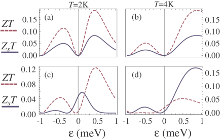
Figure 1: (color online) Spin-FOM ($Z_{s}T$, solid line, blue online) and charge-FOM ($Z_{T}$, dashed line, purple online) as a function of $\varepsilon$ at temperatures $T=2$K (left column) and $T=4$K (right column), for two values of Zeeman splitting, $\Delta B=10^{-3}$T (a-b) and $\Delta B=1.5$T (c-d) (see text for other numerical values). The spin- and charge-FOM are comparable in size, and at certain parameters spin efficiency may even exceed that of charge.

From Fig. 1 one can see that the behavior of the spin and charge FOM is similar for small Zeeman splitting, and that $Z_{s}T$ and $ZT$ are of the same order of magnitude. The situation is different for large $\Delta B$, for which at certain energies close to $\varepsilon=0$ one may obtain small $ZT$ but large $Z_{s}T$. This is due to the fact that the Zeeman splitting in that case preserves the particle-hole transport symmetry (the lack of which is responsible for charge thermo-power) but dramatically changes the transport properties of different spins, and hence increases the spin-thermopower.

Finally, we study the system at finite currents. In the bulk, a temperature gradient will inevitably induce both charge and spin voltage Uchida , and since the spin-Seebeck effect is much smaller than the charge Seebeck effect, inducing large temperature biases (to generate sizeable spin currents) would result in even larger voltage biases. In the system studied here, one can instead tune the system parameters such that there will be a large spin current but vanishing charge current.

In Fig. 2 the spin current $I_{s}$ (solid line) and charge current $I$ (dashed line) are plotted as a function of $\varepsilon$. Here the temperature $T=5$K, $\Delta B=1.5$T and we have added a constant temperature gradient $\delta T=10$K (the spin- and charge- voltage biases are zero). When the charge current vanishes (indicated by an arrow in Fig. 2) the spin current remains finite. The inset of Fig. 2 shows the dependence of the spin-current, evaluated by varying the energy $\varepsilon$ so that the charge current vanishes, as a function of the temperature bias $\delta T$. The magnitude of the spin current increases with the temperature difference, and attains significant values for realizable temperature differences, until it saturates at large temperatures (note, however, that the saturation temperature is comparable to the interaction energy $U$, and hence one expects that the sequential tunneling approximation breaks down at these temperatures). The finite spin current at large temperature difference stems from the fact that while the right lead is held at a high temperature, the temperature in the left lead is still low, allowing for differences in the tunneling rates of the different spins to be substantial. We stress that a situation of finite $I_{s}$ but vanishing $I$ can not be achieved by using only a voltage bias, but a temperature bias is needed.

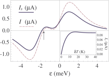
Figure 2: (color online) Spin current (solid line, blue online) and charge current (dashed line, purple online) as a function of $\varepsilon$ at a finite temperature difference $\delta T=10$K (see text for other numerical parameters). The arrow indicates the energy at which the charge current vanishes and the spin-current is finite. Inset: spin-current as a function of temperature difference, evaluated at the energy $\varepsilon$ at which the charge-current vanishes.

Our results are valid even if one considers additional single particle levels in the dot. In the limit of infinite $U$, in fact, Eq. (6) is exact for the case of equidistant levels with no Zeeman splitting. In the case with Zeeman splitting, we have numerically estimated $S_{s}/S$ for up to five levels and found that even in the presence of the additional levels $S_{s}/S\sim 1$.

The ability to couple a quantum dot to FM leads FQDFexp1 ; FQDFexp2 and to measure a local spin bias Uchida have been demonstrated experimentally. It is thus reasonable that the results presented here are accessible by future experiments. Another interesting candidate for such experiments is graphene, for which both the possibility to fabricate quantum dots Graphene1 and to bond FM leads to measure spin currents Graphene2 have been demonstrated.

We also point out that if the leads are FM, extracting the spin-current (or measuring the spin-voltage) has to be done close to the junction, at a distance shorter than the spin-diffusion length of the FM leads. Possible ways to circumvent this difficulty include the use of half-metallic leads (in which the spin-diffusion length should be very large) or to use a normal metal in contact with a thin FM layer for each lead, with the FM thin layers sandwiching the quantum dot.

We thank M. Krems and A. Sharoni for fruitful discussions. We are grateful to Yu. V. Pershin for crucial comments and to L. J. Sham for valuable remarks. This work has been funded by the DOE grant DE-FG02-05ER46204 and UC Labs.

References

- (1) G. Mahan, B. Sales and J. Sharp, Phys. Today 50, 42 (1997).
- (2) A. Majumdar, Science 303, 777 (2004).
- (3) M. Di Ventra, Electrical Transport in Nanoscale Systems (Cambridge University Press, Cambridge, 2008).
- (4) A. I. Hochbaum, R. Chen, R. D. Delgado, W. Liang, E. C. Garnett, M. Najarian, A. Majumdar and P. Yang, Nature (London) 451, 163 (2008).
- (5) A. I. Boukai, Y. Bunimovich, J. Tahir-Kheli, J.-K. Yu, W. A. Goddard III and J. R. Heath, Nature (London) 451, 168 (2008).
- (6) A. M. Lunde and K. Flensberg, J. Phys.: Condens. Matter, 17, 3879 (2005); A. M. Lunde, K. J. Flensberg and L. I. Glazman, Phys. Rev. Lett. 97, 256802 (2005).
- (7) Y. Dubi and M. Di Ventra, Nano Letters 9, 97 (2009).
- (8) C. W. J. Beenakker and A. A. M. Starling, Phys. Rev. B46, 9667 (1992); L. W. Molenkampt, A. A. M. Staring, B. W. Alphenaar, H. van Houten ana C. W. J. Beenakker, Semicond. Sci. Technol.9, 903 (1994).
- (9) M. Krawiec and K. I. Wysokinski, Phys. Rev. B73, 075307 (2006).
- (10) P. Murphy, S. Mukerjee and J. Moore, cond-mat/0805.3374 (2008).
- (11) M. Paulsson and S. Datta, Phys. Rev. B67, 241403(R) (2003); J. Koch, F. Von Oppen, Y. Oreg and E. Sela, Phys. Rev. B, 70, 195107 (2004); D. Segal, Phys. Rev. B, 72, 165426 (2005);F. Pauly, J. K. Viljas and J. C. Cuevas, Phys. Rev. B78, 035315 (2008); F. Pauly, J. K. Viljas and J. C. Cuevas, Phys. Rev. B78, 035315 (2008).
- (12) J. K. Freericks,V. Zlatic’ and A. M. Shvaika, Phys. Rev. B75, 035133 (2007); S. Mukerjee, Phys. Rev. B72, 195109 (2005); M. R. Peterson, S. Mukerjee, B. S. Shastry and J. O. Haerter, Phys. Rev. B76, 125110 (2007).
- (13) K. Uchida, S. Takahashi, K. Harii, J. Ieda, W. Koshibae, K. Ando, S. Maekawa and E. Saitoh, Nature 455, 778 (2008).
- (14) S. A. Wolf, D. D. Awschalom, R. A. Buhrman, J. M. Daughton, S. von Moln r, M. L. Roukes, A. Y. Chtchelkanova and D. M. Treger, Science 294, 1488 (2001).
- (15) See, e.g. J. Martinek, M. Sindel, L. Borda, J. Barnaś, J. König, G. Schön, and J. von Delft, Phys. Rev. Lett. 91, 247202 (2003); Y. Qi, J.-X. Zhu, S. Zhang and C. S. Ting, Phys. Rev. B 78, 045305 (2008), and references therein.
- (16) A. N. Pasupathy, R. C. Bialczak, J. Martinek, J. E. Grose, L. A. K. Donev, P. L. McEuen and D. C. Ralph, Science 306, 86 (2004).
- (17) J. R. Hauptmann, J. Paaske and P. E. Lindelof, Nature Physics 4, 373 (2008).
- (18) There should also be a term proportional to (the charge bias) which is disregarded, since it does not supply any information on the thermal efficiency.
- (19) E. Bonet, M. M. Deshmukh, and D. C. Ralph, Phys. Rev. B65, 045317 (2002).
- (20) A. G. Mal’shukov and C. S. Chu, Phys. Rev. Lett. 97, 076601 (2006).
- (21) P. M. Tedrow and R. Meservey, Phys. Rev. Lett. 26, 192 (1971).
- (22) K. Schwab, E. A. Henriksen, J. M. Worlock, and M. L. Roukes, Nature (London) 404, 974 (2000).
- (23) L. G. C. Rego and G. Kirczenow, Phys. Rev. Lett. 81, 232 (1998).
- (24) D. Segal, A. Nitzan and P. Hanggi, J. Chem. Phys. 119, 6840 (2003).
- (25) A. K. Geim and K. S. Novoselov, Nature Materials 6, 183 (2007).
- (26) N. Tombros, C. Jozsa, M. Popinciuc, H. T. Jonkman and B. J. van Wees, Nature 448, 571 (2007).