Abstract

The gravitational corrections to the gauge coupling constants of abelian and non-abelian gauge theories has been shown to diverge quadratically. Since this result will have interesting consequences, this has been analyzed by several authors from different approaches. We propose to discuss this issue from a phenomenological approach. We analyze the SU(5) gauge coupling unification and argue that the gravitational corrections to gauge coupling constants may not vanish when higher dimensional non-renormalizable terms are included in the problem.

1 Introduction

The question of gravitational corrections to the evolution of the gauge coupling constant has attracted some attention in recent times, following the seminal paper of Robinson and Wilczek [1]. They studied the one-loop quantum corrections to the running of the gauge couplings in an effective quantum theory of gravity, which is valid at energies below the Planck scale and found a quadratic divergent behavior. The character of the correction has been arrived at from a general consideration, which has been shown to have important phenomenological consequences in theories with low scale gravity [2]. However, this result has been questioned by some authors and the result has been studied from different approaches. This gravitational correction has been shown to depend on the choice of gauge in an explicit calculation [3]. They studied the abelian theory and used a parameter dependent gauge to arrive at their result. Subsequently a more general result has been obtained using a gauge invariant background field method that the gravitational corrections to the gauge couplings vanishes [4]. Following the doubts raised by these two references on the result of ref. [1], a one-loop diagrammatical calculation has been performed in the full Einstein-Yang-Mills system, which had also confirmed the vanishing of the one-loop contributions of quantum gravity to the gauge coupling evolution [5].

The quantum gravity corrections to the running of gauge couplings were calculated for pure Einstein-Yang-Mills system. Although our preliminary results show that even after including scalar fields, the diagramatic techniques would give vanishing gravitational correction, it is not clear if the general results of ref. [1] will be valid in some cases. Recently the gravitational corrections to the gauge coupling evolution has been studied including a cosmological constant and quantum gravity effect has been found to affect the running of the gauge couplings [6]. However, the one-loop contributions in the presence of a cosmological constant differs from that of ref. [1], which was obtained from a general consideration. This raises the question: what are the other factors that would make the quantum gravity effects significant?

In this article we argue from a phenomenological approach that the quantum gravity effects should be significant when higher dimensional non-renormalizable interactions are taken into consideration. Since quantizing the general theory of relativity for small fluctuations around flat space gives us a non-renormalizable field theory, we need to include an infinite set of higher dimensional counterterms. Since these terms are suppressed by appropriate powers of the Planck mass $M_{p}\sim 10^{19}$ GeV, at energies well below the Planck scale these higher dimensional terms may be considered as small perturbations in the effective theory of quantum gravity [7]. However, at the scale of grand unification these terms may not be ignored, and hence, in some version of the grand unified theories dimension-5 and dimension-6 gauge invariant terms have been included on phenomenological ground to see if these terms can change any of the conclusions for some reasonable values of the coupling constants [8]. It was found that although the minimal SU(5) grand unified theory fails to satisfy the gauge coupling unification, inclusion of the higher dimensional terms change the boundary conditions and allow gauge coupling unification at a higher scale [8, 9]. Here we point out that if the gravitational contributions to the gauge coupling evolution vanish, then the boundary conditions appearing due to the higher dimensional terms become inconsistent. We then show how the gauge coupling constants evolve from low energy to the GUT scale and satisfy the non-renormalizable operator induced matching condition at the new GUT scale, if we include gravitational corrections to the gauge couplings, which diverge quadratically near the Planck scale.

2 Effect of higher dimensional operators in SU(5) unification

Most of the grand unified theories (GUTs) with intermediate symmetry breaking scales can satisfy the experimentally observed constraints on proton lifetime ($\tau_{p}$) for the p $\rightarrow e^{+}\pi^{0}$ mode and the electroweak mixing angle $\sin^{2}\theta_{w}$

$$\tau_{p}\geq 3\times 10^{32}\leavevmode\nobreak\ {\rm yr},\leavevmode\nobreak\ \leavevmode\nobreak\ \leavevmode\nobreak\ \leavevmode\nobreak\ \leavevmode\nobreak\ \sin^{2}\theta_{w}=0.230\pm 0.005\,.$$

The minimal SU(5) and other GUTs with no intermediate symmetry breaking scale and no new particles beyond the minimal representations are ruled out as they predict significantly lower values. In other words, with the present range for the $\sin^{2}\theta_{w}$, if we evolve the three gauge coupling constants from the electroweak scale to the grand unification scale, they do not meet at a point, and hence, there is no unification. In an interesting proposal it was pointed out that since the grand unification occurs at a scale $M_{U}\geq 10^{15}$ GeV), which is close to the Planck scale, it is natural to expect that there could be significant modification to the GUT predictions by gravity-induced corrections [8]. These corrections may allow gauge coupling unification, make proton stable, give correct neutrino masses and proper charged fermion mass relations at the GUT scale, even for the minimal SU(5) GUT. In this article we include the higher dimensional terms to study the gauge coupling unification and infer that the evolution of the gauge coupling constants should be modified by the gravitational corrections.

We start with the $SU(5)$ Lagrangian and then the breaking of $SU(5)$ group into the Standard Model group $SU(3)_{C}\times SU(2)_{L}\times U(1)_{Y}$ via the Higgs field $\phi$, which transforms under the 24-dimensional adjoint representation of $SU(5)$. We write down the Lagrangian as a combination of the usual four dimensional terms plus the new higher dimensional terms which has been induced by the non-renormalizable interactions of perturbative quantum gravity. Since the couplings of these terms are not known, we cannot make any predictions at this stage, so we look for consistent solutions for a reasonable range of the unknown parameters. The SU(5) gauge invariant Lagrangian, including higher dimensional terms can be written as

$$L=L_{0}+\Sigma_{n=1}L^{(n)}$$ (1)

where

$$L_{0}=-\frac{1}{2}{\rm Tr}(F_{\mu\nu}F^{\mu\nu})$$ (2)

Where the sum is over the higher dimensional operators. For the present we shall restrict ourselves to only five- and six-dimensional operators, which are:

$$L^{(1)}=-\frac{1}{2}\frac{\eta^{(1)}}{M_{Pl}}{\rm Tr}(F_{\mu\nu}\phi F^{\mu\nu})$$ (3)

$$L^{(2)} = -\frac{1}{2}\frac{1}{M_{Pl}^{2}}\left[\eta_{a}^{(2)}{{\rm Tr}(F_{\mu\nu}\phi^{2}F^{\mu\nu})+{\rm Tr}(F_{\mu\nu}\phi F^{\mu\nu}\phi)}\phantom{a\over b}\right.$$ (4)

$$\left.+\eta_{b}^{(2)}{\rm Tr}(\phi^{2}){\rm Tr}(F_{\mu\nu}F^{\mu\nu})+\eta_{c}^{(3)}{\rm Tr}(F_{\mu\nu}\phi){\rm Tr}(F^{\mu\nu}\phi)\right]$$

where

$$F^{\mu\nu}=\partial_{\mu}A_{\nu}-\partial_{\nu}A_{\mu}-ig\left[A_{\mu},A_{\nu}\right]$$ (5)

$${(A_{\mu})^{a}}_{b}=A_{\mu}^{i}\left[\frac{\lambda_{i}}{2}\right]^{a}_{b}$$ (6)

and

$${\rm Tr}\left(\lambda_{i}\lambda_{j}\right)=\frac{1}{2}\delta_{ij}\,.$$ (7)

Here $A^{i}$ is the ith component of the gauge field, $\lambda_{i}$ is the corresponding generator and $\eta^{n}$, n=1,2,… are the unknown parameters, induced by gravitational corrections.

When the scalar $\phi$ acquires a vacuum expectation value ($vev$) and breaks the SU(5) symmetry at the GUT scale, we may replace these fields in the above expressions by its $vev$. This will give us the effective low energy theory with only dimension-4 interactions, but the effective gauge fields will be modified below the GUT scale. We may define the new physical gauge fields below the unification scale to be

$$A^{\prime}_{i}=A_{i}(1+\varepsilon_{i})^{1/2}$$ (8)

and the modified coupling constants including the higher dimensional operators as

$${\widetilde{g}_{3}}^{2}(M_{U})={g_{3}}^{2}(M_{U})(1+\varepsilon_{C})^{-1}$$ (9)

$${\widetilde{g}_{3}}^{2}(M_{U})={g_{2}}^{2}(M_{U})(1+\varepsilon_{L})^{-1}$$ (10)

$${\widetilde{g}_{1}}^{2}(M_{U})={g_{1}}^{2}(M_{U})(1+\varepsilon_{Y})^{-1}$$ (11)

The $g_{i}$ are the couplings in the absence of higher dimensional operators, whereas $\widetilde{g}_{i}$ are the physical couplings which evolve down to the lower scales. The value of the $\varepsilon^{n}$ associated with the given operator of dimension n+4 may be expressed in the following way

$$\varepsilon^{n}=\left[\frac{1}{\sqrt{15}}\frac{\phi_{0}}{M_{Pl}}\right]^{n}\eta^{(n)}$$ (12)

The vev $\phi_{0}$ is related to $M_{U}$

$$\phi_{0}=\left[\frac{6}{5\pi\alpha_{G}}\right]^{1/2}M_{U}$$ (13)

The change in the coupling constants are then related to the $\varepsilon^{n}$s through the following equations

$$\varepsilon_{C}=\varepsilon^{(1)}+{\varepsilon_{a}}^{(2)}+\frac{15}{2}{\varepsilon_{b}}^{(2)}+....$$ (14)

$$\varepsilon_{L}=-\frac{3}{2}\varepsilon^{(1)}+\frac{9}{4}{\varepsilon_{a}}^{(2)}+\frac{15}{2}{\varepsilon_{b}}^{(2)}+....$$ (15)

$$\varepsilon_{Y}=-\frac{1}{2}\varepsilon^{(1)}+\frac{7}{4}{\varepsilon_{a}}^{(2)}+\frac{15}{4}{\varepsilon_{b}}^{(2)}+\frac{7}{8}{\varepsilon_{c}}^{(2)}+....$$ (16)

This shows how the effect of higher dimensional operator modify the gauge coupling constants. The Unification scale, $M_{U}$, is now defined through the new boundary condition

$${g_{3}}^{2}(1+\varepsilon_{C})={g_{2}}^{2}(1+\varepsilon_{L})={g_{1}}^{2}(1+\varepsilon_{Y})={g_{0}}^{2}\,.$$ (17)

With this in mind, one may use the standard one loop renormalization group (RG) equations

$${\alpha_{i}}^{-1}(M_{z})={\alpha_{i}}^{-1}(M_{U})+\frac{b_{i}}{2\pi}\log\left(\frac{M_{U}}{M_{z}}\right)$$ (18)

with the beta functions $b_{1}=\frac{41}{10}$,$b_{2}=\frac{-19}{6}$,$b_{3}=-7$. We have taken $N_{f}$=3 and $N_{Higgs}$=1.

Solving the RG equations without any higher dimensional contributions yield

$$\log\left(\frac{M_{U}}{M_{z}}\right)=\frac{6}{67\alpha}\frac{1}{D}\left[{1-\frac{8}{3}\frac{\alpha}{\alpha_{s}}}+{\varepsilon_{C}-\frac{5\varepsilon_{Y}+3\varepsilon_{L}}{3}\frac{\alpha}{\alpha_{s}}}\right]$$ (19)

$$\sin^{2}{\theta_{w}}=\frac{1}{D}\left[{\sin^{2}{\theta_{w}}}^{(5)}-\frac{19}{134}\varepsilon_{C}+\frac{1}{67}\left(21+\frac{41}{2}\frac{\alpha}{\alpha_{s}}\right)\varepsilon_{L}+\frac{95}{402}\frac{\alpha}{\alpha_{s}}\varepsilon_{Y}\right]$$ (20)

$$\frac{1}{\alpha_{G}}=\frac{3}{67}\frac{1}{D}\left[\frac{11}{3\alpha_{s}}+\frac{7}{\alpha}\right]$$ (21)

$$D=1+\frac{1}{67}(11\varepsilon_{C}+21\varepsilon_{L}+35\varepsilon_{Y})$$ (22)

Where the ${\sin^{2}{\theta_{w}}}^{(5)}$ is the usual minimal SU(5) prediction

$${\sin^{2}{\theta_{w}}}^{(5)}=\frac{23}{134}+\frac{109}{201}\frac{\alpha}{\alpha_{s}}$$ (23)

In this case of minimal SU(5), the gauge coupling constants do not meet at a point, and hence, unification is not possible. We now show how this result gets modified by including higher dimensional terms.

We first consider only the following SU(5) invariant non-renormalizable (NR) (dimension five) interaction term

$$L_{NR}=-\frac{1}{2}\left(\frac{\eta}{M_{Pl}}\right){\rm Tr}(F_{\mu\nu}\phi F^{\mu\nu})\,,$$ (24)

where $\phi_{24}$ is the Higgs 24-plet, $\eta$ is a dimensionless parameter and $M_{Pl}$ is the Planck mass. Suppose the Higgs field acquires a vacuum expectation value(vev)

$$\left\langle\phi\right\rangle=\frac{1}{\sqrt{15}}\phi_{0}{\rm diag}[1,1,1,-\frac{3}{2},-\frac{3}{2}]$$ (25)

The SU(5) gauge symmetry breaks to $SU(3)_{C}\times SU(2)_{L}\times U(1)_{Y}$ at this scale because of non-invariance of the Higgs field under the SU(5) symmetry. The presence of non-renormalizable couplings modifies the usual kinetic energy terms of the $SU(3)_{c}$, $SU(2)_{L}$ and $U(1)_{Y}$ gauge boson part of the low-energy Lagrangian. The modified Lagrangian becomes

$$-\frac{1}{2}(1+\varepsilon){\rm Tr}({F_{\mu\nu}}^{(3)}{F^{\mu\nu}}^{(3)})-\frac{1}{2}(1-\frac{3}{2}\varepsilon){\rm Tr}({F_{\mu\nu}}^{(2)}{F^{\mu\nu}}^{(2)})-\frac{1}{2}(1-\frac{1}{2}\varepsilon){\rm Tr}({F_{\mu\nu}}^{(1)}{F^{\mu\nu}}^{(1)})\,,$$ (26)

where the superscripts 3,2 and 1 refer to gauge field strengths of $SU(3)$, $SU(2)$ and $U(1)$ respectively and $\varepsilon$ is defined as

$$\varepsilon=\left[\frac{1}{\sqrt{15}}\frac{\phi_{0}}{M_{Pl}}\right]\eta\,.$$ (27)

We used $\varepsilon^{(2)}=\varepsilon^{(3)}=0$ and ${\varepsilon^{(1)}}=\varepsilon=\eta{\phi}_{0}/(\sqrt{15}M_{U})$, so that $\varepsilon_{C}=\varepsilon$, $\varepsilon_{L}=-\frac{3}{2}\varepsilon$, $\varepsilon_{Y}=-\frac{1}{2}\varepsilon$. Now, using these expressions, we get

$$\frac{1}{\alpha_{G}}=\frac{11{\alpha_{s}}^{-1}+21\alpha^{-1}}{67-38\varepsilon}\,,$$ (28)

$$\log\left(\frac{M_{U}}{M_{z}}\right)=\frac{6\pi}{67-38\varepsilon}\left[\alpha^{-1}-\frac{8}{3}{\alpha_{s}}^{-1}+\left(\frac{7}{3}{\alpha_{s}}^{-1}+\alpha^{-1}\right)\varepsilon\right]$$ (29)

$$\sin^{2}{\theta_{w}}=\frac{1}{67-38\varepsilon}\left[\frac{23}{2}+\frac{109}{3}\frac{\alpha}{\alpha_{s}}-\left(41+\frac{116}{3}\frac{\alpha}{\alpha_{s}}\right)\varepsilon\right]$$ (30)

Taking the experimental values of $\alpha_{s}=0.1088$, $\alpha=1/127.54$, it is possible to obtain a consistent choice of the parameters $\varepsilon_{C}$, $\varepsilon_{L}$, $\varepsilon_{Y}$ which satisfy the constraints on $\sin^{2}{\theta_{w}}$ and $M_{U}$. But the unification scale remains low and the proton lifetime becomes less than the present experimental bound. For central value of $\sin^{2}{\theta_{w}}(=0.2333)$, we obtain $\varepsilon^{(1)}=-0.0441$ and $M_{U}=3.8\times 10^{13}$ GeV and the corresponding value of $\alpha_{G}=0.0245$. The lifetime of proton ($m_{p}$ is the mass of the proton)

$$\tau_{p}=\frac{1}{{\alpha_{G}}^{2}}\frac{{M_{U}}^{4}}{{m_{p}}^{5}}$$ (31)

then becomes too low to be consistent with experimental limits on $\tau_{p}$ for the given value of $M_{U}$. Hence, it is not possible to obtain a consistent solution with the five Dimensional operator.

Table 1: Unification in SU(5) using gravity corrections

$\epsilon_{C}$	$\epsilon_{L}$	$\epsilon_{Y}$	$M_{U}$
0.04	0.0675	0.24	$10^{17}$ GeV
0.3894	0.44	0.98	$10^{18}$ GeV
1.3894	1.445	1.98	$10^{18.6}$ GeV

If we now include both five and six dimensional terms, then there are whole range of parameters that are consistent with the values of $\sin^{2}{\theta_{w}}$, $M_{U}$ and proton lifetime. We present a few representative set of values that are consistent with proton lifetime in table 1. So, from now on we shall consider both dimension five and dimension six non-renormalizable terms for our discussion.

3 Evolution of gauge couplings including gravitational contributions

In the last section we discussed the effect of higher dimensional non-renormalizable interaction on the boundary condition, satisfied by the gauge couplings. In fact, the effective gauge couplings get modified at the time of GUT phase transition, which allows the gauge coupling unification for some parameter range. If we now start evolving the gauge coupling constants from low energy, when the effects due to the higher dimensional terms are negligible, we should be able to reach the new modified boundary condition continuously. In other words, the modified effective gauge couplings should evolve with energy in such a way that at low energy they become the usual gauge couplings. If we now assume that the gravitational corrections to the evolution of the gauge couplings vanishes, then this transition is not possible. On the other hand, if we consider that the gravitational corrections are of the quadratic nature, as recommended in ref. [1], then it is possible to continuously evolve the gauge coupling constant from the modified effective coupling near the GUT phase transition scale to the low energy experimentally observed couplings.

In this section we shall first argue how the non-renormalizable interactions could change the gravitational corrections to the gauge couplings. Then we shall demonstrate how the gauge coupling constants evolve from low energy to the unification scale in the presence of the higher dimensional contributions. Although the modified boundary condition and its effect was studied by many authors, the running of the gauge couplings from low energy to the unification scale could not be studied. This is because the running of the gauge couplings in the presence of gravitational corrections were not considered.

As the gauge boson vertex has strength $g$ and gravity couple to energy momentum with a dimensional coupling $\propto\frac{1}{M_{Pl}}$, dimensional analysis implies that the running of couplings in four dimensions will be governed by a Callan-Symanzik $\beta$ function of the form

$$\beta(g,E)=\frac{dg}{dlnE}=-\frac{b_{0}}{{4\pi}^{2}}g^{3}+a_{0}\frac{E^{2}}{{M_{Pl}}^{2}}g$$ (32)

where the first term is the non-gravitational contribution and the 2nd term is the gravitational contribution, as suggested in ref. [1]. This quadratic gravitational correction was then revisited in ref. [3, 4, 5] and it was shown that this contribution vanishes. We shall now argue that in the presence of non-renormalizable interactions, this contribution may not vanish.

Following equations 8-11, we write down the effective coupling constant at the GUT scale as

$$\widetilde{g}^{-2}=g^{-2}+C,$$ (33)

where $C$ is the contribution coming from the non-renormalizable interactions. We shall now argue that although the gauge coupling evolution may not be affected by gravitational corrections (as stated in refs. [3, 4, 5]), the evolution of $C$ is dominated by gravitational correction, and hence, it should evolve as suggested in ref. [1].

In the absence of non-renormalizable interactions and gravitational corrections, the three gauge couplings for a particular model evolve as inverse logarithm of E at one loop order. Although unification may not be achieved in case of minimal SU(5), including non-renormalizable terms (i.e., including $C$) they may get unified at a scale $\approx 10^{17-18}$ GeV. In ref. [1], it was shown that in absence of $C$, the couplings are unified near the Planck scale and the value of the couplings are zero, as shown in figure 1. The negative value of $a_{0}$ in the beta function signifies that the gravitational correction works in the direction of asymptotic freedom, i.e. it causes coupling constants to decrease at high energy (above $10^{16}$ GeV).

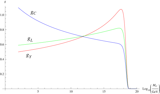
Figure 1: Evolution of the gauge coupling constants without higher dimensional terms, but including gravitational corrections [1].

The modifications to the gauge couplings arising due to non-renormalizable terms are symbolically denoted by $C$ in equation 33. To comply with the unification condition described by equation 17, the correction of each of the three coupling constants will have different weights. This would give nonzero contribution to the coupling constants unlike in ref. [3, 4, 5]. One can justify this point as follows: For the purpose of a demonstration consider the diagramatic method of ref. [5]. Here one starts with the Einstein-Yang-Mills Lagrangian

$${\cal L}_{4}={2\over\kappa^{2}}\sqrt{-g}{\mathbf{R}}-{1\over 2}\sqrt{-g}g^{\mu\rho}g^{\nu\sigma}{\rm Tr}[F_{\mu\nu}F_{\rho\sigma}]\,,$$ (34)

with the Ricci scalar ${\mathbf{R}}$. We then expand the metric in terms of the flat metric $\eta_{\mu\nu}$ and the graviton field $h_{\mu\nu}$ to write

$$g_{\mu\nu} = \eta_{\mu\nu}-\kappa h_{\mu\nu}+\kappa^{2}h_{\mu\beta}h_{\nu}^{\beta}$$

$$\sqrt{-g} = 1+{\kappa\over 2}h+{\kappa\over 8}\left(h^{2}-2h^{\alpha\beta}h_{\alpha\beta}\right)\,.$$ (35)

It is then possible to write down the propagators for this theory and explicitly calculate the one-loop diagrams to show that the gravitational corrections to the $\beta$-functions vanish [3, 4, 5]. It should be noted that the term of type $\sqrt{-g}g^{\mu\rho}g^{\nu\sigma}{\rm Tr}[F_{\mu\nu}F_{\rho\sigma}]$ (in equation 34) give contribution to the coupling constant that is quadratic in the energy [1].

If we now include the scalar fields $\Phi$ in the theory, there will be interactions of the scalar fields with the graviton field, which comes from the Lagrangian

$${\cal L}_{S}=\sqrt{-g}[D_{\mu}\Phi D_{\nu}\Phi]g^{\mu\nu}\,.$$ (36)

In this case also there seem to be cancellation of the quadratic divergences (we considered the diagrams to order $\kappa^{2}$ for the abelian case only) and there may not be any gravitational corrections to the gauge coupling evolution.

However, the inclusion of higher dimemsional non-renormalizable terms would completely change the scenario. Such non-renormalizable terms are expected in a theory that incorporates the effect of quantum gravity. In any grand unified theory, where the unification scale is only 2-3 orders of magnitude lower than the Planck scale (the proliferation of particles near the GUT scale could also lower the Planck scale [10]), such non-renormalizable terms may contribute significantly. Consider, for example, the dimension-5 term in presence of the 24-plet scalar $\phi$ of SU(5)

$${\cal L}_{5}=-{1\over 2M_{Pl}}\sqrt{-g}g^{\mu\rho}g^{\nu\sigma}{\rm Tr}[F_{\mu\nu}F_{\rho\sigma}\phi]\,.$$ (37)

For the case when $E\leq{M}_{U}$, the scalar $\phi$ acquires a $vev$ ($\langle\phi\rangle\equiv M\leavevmode\nobreak\ {\rm diag}[1,1,1,-3/2,-3/2]$),

this term would give contribution to the $C$ term in equation 33 that vary quadratically with the energy. However, to be consistent with the modified boundary condition given by equation 17, the different gauge fields with different weight factors will give nonzero contribution. It ought to be noted that the coupling constants now meet at $E\approx M_{U}$ which is lower than the Planck scale This supports our earlier inference that the gravitational corrections to the gauge couplings may not vanish when the higher dimensional interactions are included. Above the unification scale ${{M_{U}}}$, the scalar field has not acquired $vev$ and SU(5) symmetery is exact. In this regime there will be only one gauge coupling constant for entire SU(5) and it will evolve without any gravitational corrections as if the higher dimensional terms were absent.

Figure (2) shows how the coupling constants vary with energy in the presence of $C$ terms in the regime $E\leq M_{U}$. For the regime $E\geq{{M_{U}}}$, there is only one coupling constant as the exact SU(5) symmetry is restored. In this case there will be no gravitational corrections in this case as pointed out in ref. [3, 4, 5].

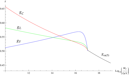
Figure 2: Evolution of the gauge coupling constants in the presence of higher dimensional terms and gravitational corrections.

4 Conclusion

The higher dimensional effective contributions has been studied in the literature, whereby the gauge coupling constants get modified near the grand unification scale. These modifications of the boundary conditions allow gauge coupling unification even for the minimal SU(5) GUT. However, the running of the modified gauge couplings have not been studied. We show that this modified gauge couplings should evolve including the gravitational corrections, otherwise the low energy gauge couplings may not be consistent with the modified boundary conditions. From this we infer that the gravitational corrections to the gauge couplings may not vanish when higher dimensional non-renormalizable interactions are included in the Einstein-Yang-Mills system.

References

- [1] S. P. Robinson and F. Wilczek, Phys. Rev. Lett. 96 231601 (2006).
- [2] I. Gogoladze, C.N. Leung, Phys. Lett. B 645, 451 (2007).
- [3] A.R. Pietrykowski, Phys. Rev. Lett. 98, 061801 (2007).
- [4] D.J. Toms, Phys. Rev. D 76, 045015 (2007).
- [5] D. Ebert, J. Plefka, and A. Rodigast, Phys. Lett. B 660, 579 (2008);
- [6] D.J. Toms, Phys. Rev. Lett. 101, 131301 (2008).
- [7] F. Donoghue, Phys. Rev. Lett. 72, 2996 (1994); Phys. Rev. D 50, 3874 (1994).
- [8] C.T. Hill, Phys. Lett. B 135, 47 (1984); Q. Shafi, and C. Wetterich, Phys. Rev. Lett. 52, 875 (1984).
- [9] M.K.Parida, P.K. Patra and A.K. Mohanty, Phys. Rev. D 39, 316 (1989); B. Brahmachari, P.K. Patra, U. Sarkar and K. Sridhar, Mod. Phys. Lett. A 8, 1487 (1993); A. Datta and S. Pakvasa and U. Sarkar, Phys. Lett. B 313, 83 (1993); A. Vayonakis, Phys. Lett. B 307, 318 (1993); T. Dasgupta, P. Mamales and P. Nath, Phys. Rev. D 52, 5366 (1995).
- [10] X. Calmet, S.D.H. Hsu and D. Reeb, Phys. Rev. Lett. 101, 171802 (2008).