A second row Parking Paradox

Abstract

We consider two variations of the discrete car parking problem where at every vertex of ${\mathbb{Z}}$ a car arrives with rate one, now allowing for parking in two lines.
a) The car parks in the first line whenever the vertex and all of its nearest neighbors are not occupied yet. It can reach the first line if it is not obstructed by cars already parked in the second line (“screening”).
b) The car parks according to the same rules, but parking in the first line can not be obstructed by parked cars in the second line (“no screening”). In both models, a car that can not park in the first line will attempt to park in the second line. If it is obstructed in the second line as well, the attempt is discarded.
We show that both models are solvable in terms of finite-dimensional ODEs. We compare numerically the limits of first and second line densities, with time going to infinity. While it is not surprising that model a) exhibits an increase of the density in the second line from the first line, more remarkably this is also true for model b), albeit in a less pronounced way.

AMS 2000 subject classification: 82C22, 82C23.

Key–Words: Car parking problem, Random sequential adsorption, Sequential frequency assignment process, Particle systems.

1 Introduction

Car parking, first considered in a mathematical way by Rényi [11] in 1958, gives rise to interesting models that in several variations have been applied in many fields of science. In the original car parking problem, unit length cars are appearing with constant rate in time and with constant density in space on the line where they try to park. A new car is allowed to park only in case there is no intersection with previously parked cars. Otherwise the attempt is rejected. Rényi proved that the density of cars has the limit $0.7475...$, the so-called parking constant. In the simplest discrete version of the car parking problem, cars of length $2$ try to park at their midpoints randomly on ${\mathbb{Z}}$. This model has been solved analytically as well [4].

This model belongs to a wider class of more complicated models of deposition with exclusion interaction. Usually such models are not analytically solvable. In physical chemistry “cars” become particles which are deposited in layers on a substrate, a process called random sequential adsorption (RSA). A variety of related models are studied. For a review of recent developments see [2]. Moreover, models with more complicated graphs e.g. (random) trees have been investigated [3],[10],[7],[6].

Multilayer variations of the model are used to describe multilayer adsorption of particles on a substrate [9] and the sequential frequency assignment process [5] which appears in telecommunication. In these papers it is also observed that the density in higher layers increases up from the first layer, which at first seems rather counterintuitive. Heuristic arguments for monotonicity of densities were found in specific models [9], but no rigorous proofs could be given yet. Moreover Privman finds numerically a scaling behavior of the density in a similar RSA model [9] with slightly different adhesion rules which is notoriously difficult to explain mathematically.

In the present paper we aim for a rigorous investigation and treat two versions of the discrete two-line car-parking problem with cars of length 2. First we describe the dynamics of the car parking process without screening and also with screening. Then we provide the solutions of these models by reducing them to closed finite dimensional systems of ODEs for densities of local patterns, see Theorems 1 and 2. That it is possible to find a finite-dimensional dynamical description is quite remarkable. It is not obvious, and in fact our method ceases to work for a three-line extension of the model without screening where an infinite system appears.

A second remarkable fact is that, even without screening, the second line density is higher than the first. Cars do not communicate or plan a common strategy and their arrival is random, but they seem to use the resources in the second line more efficiently, once they have been rejected in the first line.

2 The Dynamics

We will define a Markov jump process on the (suitably coded) occupation numbers $m=(m_{i})_{i\in{\mathbb{Z}}}\in\Omega=\{0,1,2,3\}^{\mathbb{Z}}$.

Here the spin $m_{i}$ denotes the joint occupation numbers at vertex $i$ at height $1$ and $2$. It is useful for short notation to interpret the occupation numbers at various heights as binary digits and write ordinary natural numbers. That is we write

$$m_{i}=\left\{\begin{array}[]{rl}0&\mbox{if vertex $i$ is vacant in the first and second line}\\ 1&\mbox{if vertex $i$ is occupied in the first but not in the second line}\\ 2&\mbox{if vertex $i$ is occupied in the second but not in the first line}\\ 3&\mbox{if vertex $i$ is occupied in the first and in the second line}\end{array}\right.$$

so that $m_{i}\in\{0,1,2,3\}$. The dynamics of the process is defined in terms of the generator which is given by the right hand side of the differential equation

$$\begin{split}\frac{d}{dt}\mathbb{E}^{m}f(m(t))=\sum_{k,s}\left[f(m^{s,k})-f(m)\right]c(s;m_{k-1},m_{k},m_{k+1})\end{split}$$ (2.1)

with

$$m^{s,k}_{i}=\left\{\begin{array}[]{rl}m_{i}&\mbox{if $k\neq i$ }\\ s&\mbox{if $k=i$ }\end{array}\right.$$

denoting the configuration which has been obtained by $m$ by changing the configuration in $i$ to $s$. Here ${\mathbb{E}}^{m}$ denotes the expected value with respect to the process, started at the initial configuration $m$.

Two-line parking rates

The rates are either equal to zero or one. They are $1$ precisely in the following cases.

1. $0\mapsto 1$ Adding a car in the first line at site $i$. For the model without screening we have

   $$\begin{split}c(1;0,0,0)&=c(1;2,0,0)=c(1;0,0,2)=c(1;2,0,2)=1\cr\end{split}$$ (2.2)

   Indeed, this occurs when the site itself is empty on the first and second line and the nearest neighbors are empty in the first line, see figure 1 for an example.

   Figure 1: Configurations of vertices $-1,0,$ and $1$ that allow a transition from $m_{0}=0$ to $m_{0}=1$ in the model without screening. In the model with screening only the most left configuration allows a transition to $m_{0}=1$.

   In the screening model however, cars in the second line will obstruct cars from reaching the first line. Therefore, in the screening model we have as the only nonvanishing rate

   $$\begin{split}c^{\hbox{sc}}(1;0,0,0)&=1\cr\end{split}$$ (2.3)

2. $0\mapsto 2$ Adding a car in the second line at $i$ while the first line was empty at the site

   $$\begin{split}c(2;1,0,0)&=c(2;0,0,1)=c(2;1,0,1)=1\cr\end{split}$$ (2.4)

   Indeed, this occurs when there was a supporting site $i-1$ or $i+1$ or both with one car in the first line. This is true for both models.

3. $1\mapsto 3$ Adding a car in the second line while the first line was full at the site

   $$\begin{split}c(2;0,1,0)&=1\cr\end{split}$$ (2.5)

   Indeed, this occurs when there are no obstructing cars right and left at height $2$. There can be no obstructing cars right and left at height $1$ because there could not be a car in the first line at $i$ otherwise. This is true for both models.

All other transitions are impossible.

This generator defines a Markov jump process on the infinite graph by standard theory [8], such that (2.1) holds for any local function $f:\Omega\rightarrow{\mathbb{R}}$.

3 Results

We provide a closed system of differential equations for the densities of occupied sites, involving densities of finitely many local patterns, in both models. First we need some definitions. Here and in the following we use for the densities at single sites, and triples of sites the notation

$$\begin{split}D_{t}(s)&:=P_{t}(m_{0}=s)\cr D_{t}(s_{-1},s_{0},s_{1})&:=P_{t}(m_{-1}=s_{-1},m_{0}=s_{0},m_{1}=s_{1})\cr\end{split}$$ (3.1)

Further we need the following “one-sided densities”

$$\begin{split}f_{t}(s)&:=P_{t}(m_{1}=s|N_{0}(t)=0),\quad\text{ for }s=0,1,2\cr R_{t}&:=P_{t}(m_{1}=1,m_{2}=0|N_{0}(t)=0)\end{split}$$ (3.2)

where $N_{j}(t)$ denotes the Poisson counting process of events of car arrivals at site $j$.

As our main result we show that the time-evolution of these densities gives rise to a closed ODE.

Theorem 1

Two-line Parking without Screening.
The time evolution of the probability vector $(D_{t}(0),D_{t}(1),D_{t}(2),D_{t}(3))$ obeys the following system of differential equations.

$$\begin{split}\frac{d}{dt}D_{t}(0)&=-(f_{t}(0)+f_{t}(2))^{2}e^{-t}-(2f_{t}(0)f_{t}(1)+f_{t}(1)^{2})e^{-t}\cr\frac{d}{dt}D_{t}(1)&=(f_{t}(0)+f_{t}(2))^{2}e^{-t}-D_{t}(0,1,0)\cr\frac{d}{dt}D_{t}(2)&=(2f_{t}(0)f_{t}(1)+f_{t}(1)^{2})e^{-t}\cr\frac{d}{dt}D_{t}(3)&=D_{t}(0,1,0)\cr\end{split}$$ (3.3)

with initial conditions $D_{0}(s)=1_{s=0}$, where the vector $(f_{t}(0),f_{t}(1),f_{t}(2),R_{t})$ obeys the linear ODE

$$\begin{split}\frac{d}{dt}f_{t}(0)&=-f_{t}(0)e^{-t}-f_{t}(1)e^{-t}-f_{t}(2)e^{-t}\cr\frac{d}{dt}f_{t}(1)&=f_{t}(0)e^{-t}+f_{t}(2)e^{-t}-R_{t}\cr\frac{d}{dt}f_{t}(2)&=f_{t}(1)e^{-t}\cr\frac{d}{dt}R_{t}&=f_{t}(0)(e^{-t}-te^{-2t})-f_{t}(1)te^{-2t}-R_{t}\end{split}$$ (3.4)

with initial conditions $(f_{0}(0),f_{0}(1),f_{0}(2),R_{0})=(1,0,0,0)$,
and finally, $D_{t}(0,1,0)$ is obeying the equation

$$\begin{split}\frac{d}{dt}D_{t}(0,1,0)&=f_{t}(0)^{2}e^{-t}-D_{t}(0,1,0)-2R_{t}f_{t}(0)e^{-t}-2R_{t}f_{t}(1)e^{-t}\cr\end{split}$$ (3.5)

with $D_{0}(0,1,0)=0$.

The system above can be solved numerically and the results are depicted in figure 2. As it can be seen in the right figure, surprisingly the value of $D_{t}(2)$ has a slightly higher limit than $D_{t}(1)$. This clearly means that the second line has a higher limit density of cars than the first line. This result is independently confirmed by simulations of the parking process measuring the empirical densities.

     

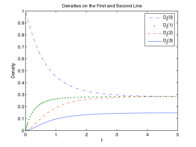
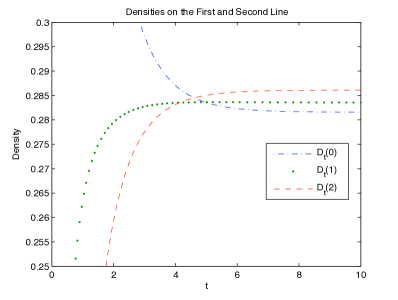
Figure 2: Numerical solution of the densities in the first and second line. The right figure zooms in on the limits of $D_{t}(1)$ and $D_{t}(2)$ to show they tend to different values.

A similar system of equations holds for the model with screening. Recall that in this model cars are not allowed to pass cars on the second line to reach a void on the first line. This results in less possibilities of filling voids of the first line than in the model treated above. In fact we can derive the ODEs of this model by simply deleting those terms in (3.4) that represent the possibility of “jumping” over a car in the second line to reach a void on the first line. So, we get

Theorem 2

Two-line Parking with Screening
The time evolution of the probability vector $(D_{t}^{sc}(0),D_{t}^{sc}(1),D_{t}^{sc}(2),D_{t}^{sc}(3))$ obeys the following system of differential equations

$$\begin{split}\frac{d}{dt}D_{t}^{sc}(0)&=-(f_{t}^{sc}(0)+f_{t}^{sc}(1))^{2}e^{-t}\cr\frac{d}{dt}D_{t}^{sc}(1)&=f_{t}^{sc}(0)^{2}e^{-t}-D_{t}^{sc}(0,1,0)\cr\frac{d}{dt}D_{t}^{sc}(2)&=(2f_{t}^{sc}(0)f_{t}^{sc}(1)+f_{t}^{sc}(1)^{2})e^{-t}\cr\frac{d}{dt}D_{t}^{sc}(3)&=D_{t}^{sc}(0,1,0)\cr\end{split}$$ (3.6)

with initial conditions $D_{0}^{sc}(s)=1_{s=0}$, where the vector $(f_{t}^{sc}(0),f_{t}^{sc}(1),f_{t}^{sc}(2),R_{t}^{sc})$ obeys the linear ODE

$$\begin{split}\frac{d}{dt}f_{t}^{sc}(0)&=-f_{t}^{sc}(0)e^{-t}-f_{t}^{sc}(1)e^{-t}\cr\frac{d}{dt}f_{t}^{sc}(1)&=f_{t}^{sc}(0)e^{-t}-R_{t}^{sc}\cr\frac{d}{dt}f_{t}^{sc}(2)&=f_{t}^{sc}(1)e^{-t}\cr\frac{d}{dt}R_{t}^{sc}&=f_{t}^{sc}(0)(e^{-t}-te^{-2t})-f_{t}^{sc}(1)te^{-2t}-R_{t}^{sc}\cr\end{split}$$ (3.7)

with initial conditions $(f_{0}^{sc}(0),f_{0}^{sc}(1),f_{0}^{sc}(2),R_{0}^{sc})=(1,0,0,0)$,
and finally, $D_{t}^{sc}(0,1,0)$ is obeying the equation

$$\begin{split}\frac{d}{dt}D_{t}^{sc}(0,1,0)&=f_{t}^{sc}(0)^{2}e^{-t}-D_{t}^{sc}(0,1,0)-2R_{t}^{sc}f_{t}^{sc}(0)e^{-t}-2R_{t}^{sc}f_{t}^{sc}(1)e^{-t}\cr\end{split}$$ (3.8)

with $D_{0}^{sc}(0,1,0)=0$.

4 Proofs of Theorem 1 and Theorem 2

The following lemmas are used to prove our theorems.

Lemma 4.1

The probability vector $(D_{t}(0),D_{t}(1),D_{t}(2),D_{t}(3))$ obeys

$$\frac{d}{dt}D_{t}(0) = -D_{t}(0,0,0)-2D_{t}(2,0,0)-D_{t}(2,0,2)-2D_{t}(1,0,0)-D_{t}(1,0,1)$$ (4.1)

$$\frac{d}{dt}D_{t}(1) = D_{t}(0,0,0)+2D_{t}(2,0,0)+D_{t}(2,0,2)-D_{t}(0,1,0)$$ (4.2)

$$\frac{d}{dt}D_{t}(2) = 2D_{t}(1,0,0)+D_{t}(1,0,1)$$ (4.3)

$$\frac{d}{dt}D_{t}(3) = D_{t}(0,1,0)$$ (4.4)

Remark: Summing over the four right hand sides we get zero, due to the fact that we have summed a probability vector. It is also interesting to check that

$$\begin{split}\frac{d}{dt}D_{t}(1)+\frac{d}{dt}D_{t}(3)&=D_{t}(0,0,0)+2D_{t}(2,0,0)+D_{t}(2,0,2)\cr\end{split}$$ (4.5)

recovers the ODE for the density in the first line.

Proof: Fix an arbitrary vertex. Let us call this vertex $0$. Starting from the dynamics (2.1) and using symmetries we have

$$\begin{split}\frac{d}{dt}D_{t}(0)&=-D_{t}(0,0,0)-2D_{t}(2,0,0)-D_{t}(2,0,2)-2D_{t}(1,0,0)-D_{t}(1,0,1)\cr\end{split}$$ (4.6)

Indeed, the first three terms correspond to adding a car in the first line, the next two terms correspond to adding a car in the second line, see figure 3.

Figure 3: List of all occupancy configurations of vertices -1, 0 and 1 in the first and second line that (may) contribute to a reduction of the proportion of $D_{t}(0)$.

The other three differential equations are derived in a similar way.

Lemma 4.2

The triple site densities $D_{t}(s,0,s^{\prime})$ and the one-sided densities as defined in LABEL:def:Dt and 3.2 respectively are related in the following way

$$\begin{split}D_{t}(s,0,s^{\prime})&=f_{t}(s)f_{t}(s^{\prime})e^{-t}\cr\end{split}$$ (4.7)

for $(s,s^{\prime})\in\{(0,0),(0,1),(1,0),(1,1),(2,2)\}$.

Proof: We note that for the mentioned choices of $(s,s^{\prime})$ conditioning on non-arrival at zero does not change the probability, that is

$$\begin{split}D_{t}(s,0,s^{\prime})&=P_{t}(m_{-1}=s,m_{0}=0,m_{1}=s^{\prime},N_{0}(t)=0)\cr&=P_{t}(m_{-1}=s,m_{0}=0,m_{1}=s^{\prime}|N_{0}(t)=0)e^{-t}\cr\end{split}$$ (4.8)

In the next step we note that, conditional on the event that no car has arrived at the site $0$, the dynamics for the two sides that are emerging from $0$ is independent. Consequently we have

$$\begin{split}&P_{t}(m_{-1}=s,m_{0}=0,m_{1}=s^{\prime}|N_{0}(t)=0)\cr&=P_{t}(m_{1}=s|N_{0}(t)=0)P_{t}(m_{1}=s^{\prime}|N_{0}(t)=0)\cr\cr\end{split}$$ (4.9)

This concludes the proof of the Lemma. $\hfill\Box$

Next we look at the time-evolution of the “one-sided densities”.

Lemma 4.3

The vector $(f_{t}(0),f_{t}(1),f_{t}(2),R_{t})$ obeys the ODE

$$\begin{split}\frac{d}{dt}f_{t}(0)&=-f_{t}(0)e^{-t}-f_{t}(1)e^{-t}-f_{t}(2)e^{-t}\cr\frac{d}{dt}f_{t}(1)&=f_{t}(0)e^{-t}+f_{t}(2)e^{-t}-R_{t}\cr\frac{d}{dt}f_{t}(2)&=f_{t}(1)e^{-t}\cr\frac{d}{dt}R_{t}&=f_{t}(0)(e^{-t}-te^{-2t})-f_{t}(1)te^{-2t}-R_{t}\end{split}$$ (4.10)

with initial conditions $f_{t=0}(s)=1_{s=0}$ and $R_{t=0}=0$.

Remark 1: Note that combining the equations of $\frac{d}{dt}f_{t}(0)$ and $\frac{d}{dt}f_{t}(2)$ readily gives

$$f_{t}(0)+f_{t}(2)=\exp(e^{-t}-1)$$ (4.11)

which is a known result for the first line in a semi-infinite chain [4].

Remark 2: Note also that because $R_{t}:=P_{t}(m_{1}=1,m_{2}=0|N_{0}(t)=0)$ we have in fact $R_{t}=\frac{d}{dt}f_{t}(3)$.

Proof: To derive ODEs for these densities we employ the generator of the process, while putting the term at the site $0$ to sleep, and correspondingly the spin at zero to be the constant $m_{0}=0$. For the first quantity we get

$$\begin{split}\frac{d}{dt}f_{t}(0)&=\frac{d}{dt}P_{t}(m_{1}=0|N_{0}(t)=0)\cr&=-P_{t}(m_{1}=0,m_{2}=0|N_{0}(t)=0)-P_{t}(m_{1}=0,m_{2}=2|N_{0}(t)=0)\cr&~{}-P_{t}(m_{1}=0,m_{2}=1|N_{0}(t)=0)\cr&=-P_{t}(m_{1}=0,m_{2}=0|N_{0}(t)=0,N_{1}(t)=0)e^{-t}\cr&~{}-P_{t}(m_{1}=0,m_{2}=2|N_{0}(t)=0,N_{1}(t)=0)e^{-t}\cr&-P_{t}(m_{1}=1|N_{0}(t)=0)e^{-t}\cr&=-P_{t}(m_{1}=0|N_{0}(t)=0)e^{-t}-P_{t}(m_{1}=2|N_{0}(t)=0)e^{-t}\cr&-P_{t}(m_{1}=1|N_{0}(t)=0)e^{-t}\cr&=-f_{t}(0)e^{-t}-f_{t}(1)e^{-t}-f_{t}(2)e^{-t}\cr\cr\end{split}$$ (4.12)

Next we have

$$\begin{split}\frac{d}{dt}f_{t}(1)&=\frac{d}{dt}P_{t}(m_{1}=1|N_{0}(t)=0)\cr&=P_{t}(m_{1}=0,m_{2}=0|N_{0}(t)=0)+P_{t}(m_{1}=0,m_{2}=2|N_{0}(t)=0)\cr&-P_{t}(m_{1}=1,m_{2}=0|N_{0}(t)=0)\cr&=f_{t}(0)e^{-t}+f_{t}(2)e^{-t}-R_{t}\cr\cr\end{split}$$ (4.13)

and

$$\begin{split}\frac{d}{dt}f_{t}(2)&=\frac{d}{dt}P_{t}(m_{1}=2|N_{0}(t)=0)\cr&=P_{t}(m_{1}=0,m_{2}=1|N_{0}(t)=0)\cr&=P_{t}(m_{1}=1|N_{0}(t)=0)e^{-t}\cr\end{split}$$ (4.14)

Finally, we get

$$\begin{split}\frac{d}{dt}R_{t}&=\frac{d}{dt}P_{t}(m_{1}=1,m_{2}=0|N_{0}(t)=0)\cr&=P_{t}(m_{1}=0,m_{2}=0|N_{0}(t)=0)-P_{t}(m_{1}=1,m_{2}=0|N_{0}(t)=0)\cr&-P_{t}(m_{1}=1,m_{2}=0,m_{3}=0|N_{0}(t)=0)\cr&-P_{t}(m_{1}=1,m_{2}=0,m_{3}=1|N_{0}(t)=0)\end{split}$$ (4.15)

Using conditioning on non-arrival again we get

$$\begin{split}&\frac{d}{dt}P_{t}(m_{1}=1,m_{2}=0|N_{0}(t)=0)\cr&=P_{t}(m_{1}=0|N_{0}(t)=0)e^{-t}-P_{t}(m_{1}=1,m_{2}=0|N_{0}(t)=0)\cr&-P_{t}(m_{1}=1|N_{0}(t)=0,N_{2}(t)=0)P_{t}(m_{1}=0|N_{0}(t)=0)e^{-t}\cr&-P_{t}(m_{1}=1|N_{0}(t)=0,N_{2}(t)=0)P_{t}(m_{1}=1|N_{0}(t)=0)e^{-t}\cr\end{split}$$ (4.16)

Clearly we have

$$\begin{split}&P_{t}(m_{1}=1|N_{0}(t)=0,N_{2}(t)=0)=te^{-t}\end{split}$$ (4.17)

because there is precisely one car at $1$ if and only if precisely one car arrived conditioning on no cars at $0$ and $2$. This shows that the last ODE is correct and concludes the proof of the lemma.$\hfill\Box$

The only remaining term whose time-evolution we need to consider is $D_{t}(0,1,0)$.

Lemma 4.4

$D_{t}(0,1,0)$ is a solution of the differential equation

$$\begin{split}\frac{d}{dt}D_{t}(0,1,0)&=f_{t}(0)^{2}e^{-t}-D_{t}(0,1,0)-2R_{t}f_{t}(0)e^{-t}-2R_{t}f_{t}(1)e^{-t}\cr\end{split}$$ (4.18)

Proof: We note that

$$\begin{split}\frac{d}{dt}D_{t}(0,1,0)&=D_{t}(0,0,0)-D_{t}(0,1,0)-2D_{t}(0,1,0,0)-2D_{t}(0,1,0,1)\cr\cr\end{split}$$ (4.19)

The first term is for adding a car at the central site from the vacuum, the second for adding a car at the central site at height one. The last two terms are for adding a car to the right of the central site. As we already know we have

$$\begin{split}D_{t}(0,0,0)=P_{t}(m_{1}=0|N_{0}(t)=0)^{2}e^{-t}\cr\end{split}$$ (4.20)

Using conditioning on non-arrival at $2$ we get, by reflection invariance

$$\begin{split}D_{t}(0,1,0,0)&=P_{t}(m_{1}=1,m_{2}=0|N_{0}(t)=0)P_{t}(m_{1}=0|N_{0}(t)=0)e^{-t}\cr&=R_{t}f_{t}(0)e^{-t}\end{split}$$ (4.21)

For the last term we get in the same way

$$\begin{split}D_{t}(0,1,0,1)&=P_{t}(m_{1}=1,m_{2}=0|N_{0}(t)=0)P_{t}(m_{1}=1|N_{0}(t)=0)e^{-t}\cr&=R_{t}f_{t}(1)e^{-t}\cr\end{split}$$ (4.22)

$\hfill\Box$

Proof of Theorem 1: Combining the results of lemma 4.1, 4.2, 4.3 and 4.18 proves Theorem 1. $\hfill\Box$

Proof of Theorem 2: The proof follows from Theorem 1 by deleting every term that represents the possibility of skipping a second line car to reach a void in the first line. This results in deleting $f_{t}(2)e^{-t}$ from the first two equations of 4.3, and $D_{t}(2,0,0)$ and $D_{t}(2,0,2)$ from 4.1 and 4.2. $\hfill\Box$

     

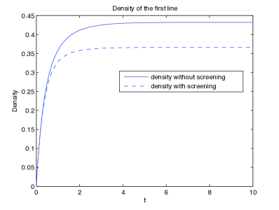
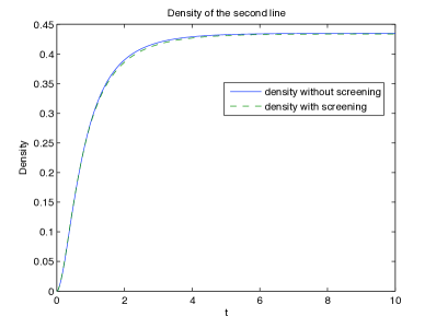
Figure 4: Densities of the first and second line.

5 Conclusion

We introduced two extensions of the classic parking problem to a two-line model i.e. a model with screening and a model without screening. For both models we derived closed systems of finite-dimensional ODEs from which the time-evolution of the densities in the first and second line can be obtained. Interestingly, the numerical solution of the ODE shows that the final densities in the second line are higher than those in the first line, for both models. The increase factor in the model without screening is approximately

$$I=\lim_{t\rightarrow\infty}\frac{D_{t}(2)+D_{t}(3)}{D_{t}(1)+D_{t}(3)}\approx\frac{0.434868}{0.432332}\approx 1.006$$

It is known by analytical computations [4] that $D_{t}(1)+D_{t}(3)$ approaches $(1-e^{-2})/2\approx 0.432332$ for large $t$, which provides a checkup for the numerics. In the screening model we find

$$I_{sc}=\lim_{t\rightarrow\infty}\frac{D_{t}^{sc}(2)+D_{t}^{sc}(3)}{D_{t}^{sc}(1)+D_{t}^{sc}(3)}\approx\frac{0.433896}{0.366475}\approx 1.184$$

In other words, in both models the cars seem to exploit the resources in the second line in a (slightly) more efficient way than in the first line.

References

• [1]
• [2] A. Cadilhe, N. A. M. Araujo, V. Privman, Random Sequential Adsorption: From Continuum to Lattice and Pre-Patterned Substrates, J. Phys. Cond. Matter  19, (2007), Article 065124,
• [3] A. Cadilhe, V. Privman, Random Sequential Adsorption of Mixtures of Dimers and Monomers on a Pre-Treated Bethe Lattice, Modern Phys. Lett. B 18, (2004), pp. 207–211.
• [4] R. Cohen, H. Reiss, Kinetics of Reactant Isolation I. One-Dimensional Problems, J. Chem. Phys. 38, no. 3, (1963), pp. 680–691.
• [5] H.G. Dehling, S.R. Fleurke, The Sequential Frequency Assignment Process, Proc. of the 12th WSEAS Internat. Conf. on Appl. Math. Cairo, Egypt, (2007), pp. 280–285
• [6] H.G. Dehling, S.R. Fleurke, C. Külske, Parking on a Random Tree, J. Stat. Phys. 133, no. 1, (2008), pp. 151–157.
• [7] R. Gouet, A. Sudbury, Blocking and Dimer Processes on the Cayley Tree, J. Stat. Phys. 130 (2008), pp.  935–955.
• [8] T.M. Liggett, Interacting Particle Systems, Springer, New York, (1985).
• [9] P. Nielaba, V. Privman, Multilayer Adsorption with Increasing Layer Coverage. Phys. Rev. A 45, (1992), pp. 6099–6102.
• [10] M.D. Penrose, A. Sudbury, Exact and Approximate Results for Deposition and Annihilation Processes on Graphs. Ann. Appl. Prob. 15, no. 1B, (2005), pp. 853–889.
• [11] A. Rényi, On a One-dimensional Problem Concerning Random Space-filling, Publ. Math. Inst. Hung. Acad. Sci. 3, (1958), pp. 109–127.