Positive maps, majorization, entropic inequalities, and detection of entanglement

Abstract

In this paper, we discuss some general connections between the notions of positive map, weak majorization and entropic inequalities in the context of detection of entanglement among bipartite quantum systems. First, basing on the fact that any positive map $\Lambda:M_{d}(\mathbb{C})\to M_{d}(\mathbb{C})$ can be written as the difference between two completely positive maps $\Lambda=\Lambda_{1}-\Lambda_{2}$, we propose a possible way to generalize the Nielsen–Kempe majorization criterion. Then we present two methods of derivation of some general classes of entropic inequalities useful for the detection of entanglement. While the first one follows from the aforementioned generalized majorization relation and the concept of the Schur–concave decreasing functions, the second is based on some functional inequalities. What is important is that, contrary to the Nielsen–Kempe majorization criterion and entropic inequalities, our criteria allow for the detection of entangled states with positive partial transposition when using indecomposable positive maps. We also point out that if a state with at least one maximally mixed subsystem is detected by some necessary criterion based on the positive map $\Lambda$, then there exist entropic inequalities derived from $\Lambda$ (by both procedures) that also detect this state. In this sense, they are equivalent to the necessary criterion $[I\otimes\Lambda](\varrho_{AB})\geq 0$. Moreover, our inequalities provide a way of constructing multi–copy entanglement witnesses and therefore are promising from the experimental point of view. Finally, we discuss some of the derived inequalities in the context of recently introduced protocol of state merging and possibility of approximating the mean value of a linear entanglement witness.

1 Introduction

Due to its interesting applicability, entanglement (see e.g. [1]) is still one of the most interesting topics in modern physics. Following [2], we call a state describing some finite–dimensional bipartite physical system $A$ and $B$ entangled if it cannot be written as a mixture of product states. More precisely, $\varrho_{AB}$ is called entangled if it does not admit the following decomposition:

$$\varrho_{AB}=\sum_{i}p_{i}\varrho_{A}^{(i)}\otimes\varrho_{B}^{(i)},\qquad p_{i}\geq 0,\qquad\sum_{i}p_{i}=1,$$ (1)

where $\varrho_{A(B)}^{(i)}$ are density matrices representing subsystems $A$ and $B$. In the case when $\varrho_{AB}$ can be written in the above form, it is called separable or classically correlated.

One of the most important problems the scientists have to face is that there is no simple way of deciding if a given state $\varrho_{AB}$ is entangled or not. The general problem of separability remains unresolved despite the fact that huge effort has been expended so far to invent stronger and easier to apply separability criteria (see e.g. [3, 4, 5, 6, 7, 8, 9, 10, 11, 12, 13, 14, 15] and the recent review on the detection of entanglement [16]). The task becomes even harder since most of the invented mathematical criteria are not directly applicable experimentally. In general, despite the case of pure states (see [17]) and arbitrary two–qubit states (see [18]), there is no unambiguous method for deciding about separability that is promising from the experimental point of view. Therefore, it is still desirable to look for separability criteria giving, on the one hand, mathematical possibility of detecting entanglement and, on the other hand, allowing for future experimental realizations.

Still, one of the most significant separability criteria, but in general not directly realizable in experiment, are those based on positive maps. It was pointed out first for the partial transposition in [3] and then generally in [5] that a positive map can serve as a necessary separability criterion. That is, whenever $\varrho_{AB}$ is separable, the operator inequality

$$[I\otimes\Lambda](\varrho_{AB})\geq 0$$ (2)

holds for all positive but not completely positive maps $\Lambda$. Here, by $I$ we denoted an identity map acting on the first subsystem. In fact, even a stronger statement is true [5], i.e. $\varrho_{AB}$ is separable if and only if condition (2) is satisfied for all positive maps $\Lambda$. Exemplary maps serving commonly for the detection of entanglement are the reduction map [19, 20] $\Lambda_{R}=\Lambda_{\mathrm{Tr}}-I$ with $\Lambda_{\mathrm{Tr}}(X)=\Tr(X)\mathbbm{1}_{d}$ and the transposition map (hereafter denoted by $T$) [3, 5]. Interestingly, it was shown in [5] that in the case of the $2\otimes 2$ and $2\otimes 3$ system the transposition map completely solves the separability problem, as in this case $[I\otimes T](\varrho_{AB})\equiv\varrho^{\Gamma}_{AB}\geq 0$ is a necessary and sufficient condition for separability. Though the criteria cannot be applied directly in experiment, some indirect methods were pointed out in a series of papers [21].

On the other hand, there also exist criteria that seem to be promising from the experimental point of view and can be given clear physical interpretation. Among others are the so–called entropic inequalities. Their meaning for detection of entanglement was first pointed out in [22], where it was shown that for separable states the von Neumann conditional entropy satisfies $S(B|A;\varrho_{AB})\equiv S(\varrho_{AB})-S(\varrho_{A(B)})\geq 0$, where $S$ denotes the von Neumann entropy $S(\sigma)=-\Tr\sigma\log\sigma$. This means that in the case of separable states the whole system is more disordered than its subsystems. However, the nonnegativity of conditional entropy does not have to hold for all quantum states (as it is easily seen in the case of pure entangled states). This phenomenon found its explanation in [23], where the conditional von Neumann entropy was interpreted as the cost of merging of a bipartite state. The fact that for some entangled states this quantity can be negative is one of the basic features of quantum communication.

Further, in a series of papers [4, 24, 25, 26], the property that for separable states the whole system is more disordered than the subsystems was formalized in terms of other disorder measures, for instance the quantum version of the Renyi entropy [27] (or equivalently the Tsallis entropy [28]). This led to inequalities of the form

$$S_{\alpha}^{R}(\varrho_{A(B)})\leq S_{\alpha}^{R}(\varrho_{AB})\qquad(\alpha\geq 0)$$ (3)

with $S^{R}_{\alpha}(\sigma)=[1/(1-\alpha)]\log\Tr\sigma^{\alpha}$ (see e.g. [29]). Applicability in the detection of entanglement among many particular examples of quantum states were investigated in the literature (see e.g. [30, 31]). Also, other entropic functions were studied in this context [32].

This disorder rule was also connected to a more general disorder measure based on the concept of majorization (the definition of majorization will be given in Section 2). In [7], it was shown that if $\varrho_{AB}$ is separable, then the following holds:

$$\lambda(\varrho_{A})\succ\lambda(\varrho_{AB})\quad\wedge\quad\lambda(\varrho_{B})\succ\lambda(\varrho_{AB}),$$ (4)

where $\lambda(\varrho_{AB})$ and $\lambda(\varrho_{A(B)})$ denote vectors consisting of eigenvalues of $\varrho_{AB}$ and $\varrho_{A(B)}$, respectively (note that one has to add zeros to $\lambda(\varrho_{A(B)})$ to have the same dimension as $\lambda(\varrho_{AB})$).

The advantage of the entropic inequalities lies in the fact that they can be measured experimentally. More precisely, since they can be rewritten as

$$\Tr\varrho_{A(B)}^{\alpha}\geq\Tr\varrho^{\alpha}_{AB}\qquad(\alpha\in[1,\infty))$$ (5)

$$\Tr\varrho_{A(B)}^{\alpha}\leq\Tr\varrho^{\alpha}_{AB}\qquad(\alpha\in[0,1)),$$ (6)

they lead, for integer $\alpha$, to multicopy entanglement witnesses on $\alpha$ copies of $\varrho_{AB}$ [33]. For $\alpha=2$, this fact has already been already applied experimentally [34, 35] and a possible generalization to $n$–qubit states was considered in [36].

On the other hand, both criteria (majorization relations and entropic inequalities) were shown to follow from the reduction criterion [26, 37]. This means that they are useless in detecting entangled states with positive partial transposition (PPT) [38], since the reduction map is decomposable, and in general weak. In a series of two papers [39, 40], the question about other entropic or entropic–like inequalities that could detect bound entanglement and could be realized experimentally was posed. The fact that the reduction criterion map leads to some scalar criteria suggests that it should be also possible to get some entropic–like inequalities from other maps, including indecomposable ones. Using the fact that any positive map $\Lambda:M_{d}(\mathbb{C})\to M_{d}(\mathbb{C})$ may be written as $\Lambda=\Lambda_{1}-\Lambda_{2}$ with $\Lambda_{i}$ ($i=1,2$) being two completely positive maps, the authors derived in [40] a class of inequalities efficiently detecting entanglement. However, these inequalities can be applied only to states fulfilling some commutation relations.

The purpose of the present paper is to reexamine the question about the possibility of deriving entropic–like inequalities from any positive map, not only the reduction one, but without any additional assumptions on the state. Analogously, we ask if there are some majorization criteria following from any positive map. This in turn, by the concept of the Schur–convex functions, could give a general method of deriving scalar inequalities appropriate for experimental realization. In what follows we show that it is possible to get submajorization relations following from positive maps. Then, we provide two methods allowing for the derivation of entropic inequalities. The first one is a simple consequence of the submajorization relations, while the second one is a continuation of the results from [40]. Both constructions give separability tests allowing for detection of PPT entangled states. Interestingly, for states with one of the subsystems being in a maximally mixed state the derived inequalities are in some sense equivalent to the necessary condition based on the positive map from which they were derived. Finally, the particular inequalities derived using the second method can be given some physical meaning in the context of state merging and approximation of a mean value of a linear entanglement witness.

The paper is organized as follows: Section 2 contains various definitions concerning majorization, week majorization, positive maps and related concepts. The reader familiar with the subject matter can move straight to Section 3, where the inequalities are presented together with some special cases and comments. In Section 4, we analyze the effectiveness of the inequalities as a separability criterion. A summary of obtained results and some open questions are given in section 5.

2 Definitions

2.1 Majorization and the Schur–concave functions

In what follows we shall often refer to the notion of majorization. It is therefore desirable to recall the definition and some concepts closely related to it. The meaning of majorization in physics has already been recognized (see e.g. [41] and references therein). Recently, majorization found its applications also in issues closely related to quantum information theory (see e.g. [7, 42, 43]).

All the concepts appearing in this subsection can be found e.g. in [44, 45]. Let then $x$ be a vector from $\mathbb{R}^{d}$ and $x^{\downarrow}=(x_{0}^{\downarrow},\ldots,x^{\downarrow}_{d-1})\in\mathbb{R}^{d}$ denote a vector consisting of coordinates of $x$ put in decreasing order, i.e. $x_{0}^{\downarrow}\geq x_{1}^{\downarrow}\geq\ldots\geq x_{d-1}^{\downarrow}$. We say that $x$ majorizes $y$, which we write as $x\succ y$, if the conditions

$$\sum_{i=0}^{k}x_{i}^{\downarrow}\geq\sum_{i=0}^{k}y^{\downarrow}_{i}$$ (7)

hold for any $k=0,\ldots,d-2$ and

$$\sum_{i=0}^{d-1}x_{i}^{\downarrow}=\sum_{i=0}^{d-1}y^{\downarrow}_{i}.$$ (8)

However, if in the last condition one replaces equality with inequality ‘$\geq$’, then we say that $x$ weakly majorizes (or submajorizes) $y$, which we shall denote by $x\,\,{}_{w}\!\!\succ y$.

The notions of majorization and weak majorization are strictly connected to the notion of doubly stochastic and doubly substochastic matrices. Let then $S$ denote some $d\times d$ matrix. We say that $S=(S_{ij})$ is a doubly stochastic (substochastic) matrix if $S_{ij}\geq 0$ and the sum of all elements in any row and column equals one (is less than or equal to one). Using the above notions, we can reformulate the concept of majorization as follows (see e.g. [44]).

Fact 1. Let $x,y\in\mathbb{R}^{d}$. Then $x\succ y$ ($x\,\,{}_{w}\!\!\succ y$) if and only if there exists such a doubly stochastic (doubly substochastic) matrix $S$ that

$$y=Sx.$$ (9)

Another notion useful for further considerations and strictly connected with majorization is the Schur–convex function. We say that a real–valued function $\phi:\mathcal{I}^{d}\to\mathbb{R}$ ($\mathcal{I}\subseteq\mathbb{R}$ denotes some open interval) is Schur–convex if the following implication holds:

$$x\succ y\quad\Rightarrow\quad\phi(x)\geq\phi(y).$$ (10)

If the inequality in the above is reversed, we say that $\phi$ is Schur–concave. There is an easy–to–apply tool allowing us to decide if a given function $\phi$ is Schur–convex (concave). Namely, $\phi:\mathcal{I}^{d}\to\mathbb{R}$ is Schur–convex if and only if it is symmetric and fullfils the following condition:

$$(x_{i}-x_{j})\left(\frac{\partial\phi(x)}{\partial x_{i}}-\frac{\partial\phi(x)}{\partial x_{j}}\right)\geq 0$$ (11)

for any $i\neq j$ (see e.g. [45]). Once again, if the inequality in the above is reversed, the function $\phi$ is Schur–concave. (Notice that if $\phi$ is symmetric one does not have to check the above condition for all $i$ and $j$. It suffices to check it for some pair $i\neq j$.)

The last definition we give in this subsection deals with the monotonicity of a multi–variable function. We say that a $d$–argument function $\phi$ is increasing (decreasing) if for $x,y\in\mathbb{R}^{d}$ and $x\geq y$ one has $\phi(x)\geq\phi(y)$ ($\phi(x)\leq\phi(y)$). Here the ordering relation $x\geq y$ means that $x_{i}\geq y_{i}$ for any $i=0,\ldots,d-1$. If the above inequalities are strict we call a function strictly increasing (decreasing).

2.2 Positive maps

Finally, we introduce the concepts of positive and completely positive map and discuss some of their properties. Let $\Lambda:M_{d}(\mathbb{C})\to M_{d}(\mathbb{C})$ denote a linear map. We say that $\Lambda$ is positive if, acting on a positive element of $M_{d}(\mathbb{C})$, it returns a positive matrix. We say that $\Lambda$ is completely positive if the extended map $I_{k}\otimes\Lambda$ is positive for any natural $k$. Here by $I_{k}:M_{k}(\mathbb{C})\to M_{k}(\mathbb{C})$ we denoted the identity map. A more detailed characterization of positive and completely positive maps can be found, e.g. in [46, 47]. As already stated, any positive but not completely positive map constitutes a necessary separability criterion for finite bipartite quantum systems. Moreover, we say that a positive map $\Lambda$ is decomposable (indecomposable) if it can (cannot) be written as a sum of a completely positive map and a completely positive map composed with transposition map. What is important here is that separability criteria based on decomposable positive maps cannot detect PPT entangled states. Only indecomposable maps have this advantage.

On the other hand, any positive map on finite–dimensional matrix algebra can be written as the difference of two completely positive maps $\Lambda_{1}$ and $\Lambda_{2}$ (see e.g. [48]), i.e.

$$\Lambda=\Lambda_{1}-\Lambda_{2}.$$ (12)

Then the necessary condition for separability of $\varrho_{AB}$ based on some particular positive map $\Lambda$ reads:

$$[I\otimes\Lambda_{1}](\varrho_{AB})\geq[I\otimes\Lambda_{2}](\varrho_{AB}).$$ (13)

Finally, it should be also reminded that any completely positive map $\Lambda_{CP}:M_{d}(\mathbb{C})\to M_{d}(\mathbb{C})$ can be written as [47, 49]

$$\Lambda_{CP}(\cdot)=\sum_{i=1}^{\kappa}V_{i}(\cdot)V_{i}^{\dagger},$$ (14)

where $V_{i}$ are some linearly independent $d\times d$ matrices. The parameter $\kappa$ corresponding to the smallest number of operators $V_{i}$ in (14) is called a minimal length of $\Lambda$ [50]. In this way any positive map on a finite matrix algebra is characterized by two numbers $\kappa_{1}$ and $\kappa_{2}$ corresponding to completely positive maps $\Lambda_{1}$ and $\Lambda_{2}$ in its decomposition. The decomposition corresponding to minimal $\kappa_{1}+\kappa_{2}$ will be called a minimal decomposition. As we shall see later, the efficiency of our inequalities in detecting entanglement strongly depends on the choice of $\Lambda_{1}$ and $\Lambda_{2}$ in equation (12).

For simplicity, in further considerations, we shall be denoting an extended map $I\otimes\Lambda_{i}$ by $\Theta_{i}$ $(i=1,2)$ and $\varrho_{AB}$ by $\varrho$ whenever it does not lead to confusion.

3 Inequalities

Now we are ready to provide two constructions of entropic–like inequalities. The first method goes through the weak majorization relations generalizing the famous majorization criterion by Nielsen and Kempe [7], while the second one is direct in the sense that beginning with an operator inequality (13), we prove some functional inequality which in case of reduction map reproduces the standard entropic criterion. Before that, in the following subsection, we will briefly recall some of the results of [39, 40].

3.1 Already known entropic–like inequalities going beyond the standard ones

As mentioned previously the standard entropic inequalities, though they possess a physical interpretation, are unable to detect PPT entangled states. This is because they follow from the reduction criterion [26], which is in general weaker than the criterion based on transposition. The question about the possibility of constructing some stronger inequalities resembling the entropic ones, using other positive maps (also indecomposable), has been recently addressed in [39, 40]. Firstly, in [39] it was shown that using the Breuer–Hall map [51, 52]:

$$\Lambda_{BH}^{U}(X)=\Tr(X)\mathbbm{1}_{d}-X-\tau^{U}(X)\qquad(X\in M_{d}(\mathbb{C})),$$ (15)

where $\tau^{U}(X)=UX^{T}U^{\dagger}$ with $U$ denoting some antisymmetric matrix $(U^{T}=-U)$ obeying $U^{\dagger}U\leq\mathbbm{1}_{d}$, one can derive inequalities efficiently detecting PPT states. However, the inequalities work only when some commutation relations are satisfied by the investigated state. For instance, assuming that $\varrho$ is separable and that the commutation relation $[\varrho,\varrho_{A}\otimes\mathbbm{1}_{d}]=0$ holds, the following inequality was derived in [39]:

$$\Tr\varrho_{A}^{\alpha}\geq\frac{1}{2}\left\{\Tr\left[\varrho(\varrho+\tau_{B}^{U}(\varrho))^{\alpha-1}\right]+\Tr\left[\varrho(\varrho-\tau_{B}^{U}(\varrho))^{\alpha-1}\right]\right\}$$ (16)

with $\alpha\geq 1$. Assuming further that $[\varrho,\tau_{B}^{U}(\varrho)]=0$, we can obtain from the above

$$\Tr\varrho_{A}^{\alpha}\geq\Tr\varrho^{\alpha}+\sum_{k=1}^{\lfloor(\alpha-1)/2\rfloor}\left(\begin{array}[]{c}\alpha-1\\ 2k\end{array}\right)\Tr\left\{\varrho^{\alpha-2k}[\tau_{B}^{U}(\varrho)]^{2k}\right\}.$$ (17)

In both inequalities $\varrho_{A}=\Tr_{B}\varrho$ and $\tau_{B}^{U}$ denotes the map $\tau^{U}$ applied to the second subsystem. Comparing the above to the standard entropic inequalities (5), it is clear that they are stronger, since on the right–hand hand side we have an additional nonnegative term. Moreover, it was pointed out in [39] that such inequalities can detect PPT entangled states in some physical systems.

In [40], the authors posed a question about some more general inequalities following from any positive map $\Lambda$. For instance, the following inequalities:

$$\Tr\varrho^{\alpha}\left([I\otimes\Lambda_{1}](\varrho)\right)^{\beta}\geq\Tr\varrho^{\alpha}\left([I\otimes\Lambda_{2}](\varrho)\right)^{\beta}\qquad(\beta\geq 0)$$ (18)

and

$$\Tr\varrho^{\alpha}\left([I\otimes\Lambda_{1}](\varrho)\right)^{\beta}\leq\Tr\varrho^{\alpha}\left([I\otimes\Lambda_{2}](\varrho)\right)^{\beta}\qquad(\beta\in[-1,0)),$$ (19)

were derived, both for $\alpha\geq 0$. It should also be explicitly stated than in the case of the second inequality (19) one has to remember that both operators $[(I\otimes\Lambda_{i})(\varrho)]^{\beta}$ have to be ‘sandwiched’ with the projector onto the support of $[I\otimes\Lambda_{2}](\varrho)$ (this can always be done during the derivation of this inequality, cf proof of Theorem 2) to avoid the problems of inverse of matrices that are not of full rank. This means that on the right–hand side one can take the pseudoinverse of $[I\otimes\Lambda_{2}](\varrho)$.

Unfortunately, to prove both inequalities (18) and (19) (except for the case $\beta\in[0,1)$), one has to assume that $[[I\otimes\Lambda_{2}](\varrho),\varrho]=0$; however, as discussed in [40], for many of the known positive (even indecomposable) maps, $\Lambda_{2}$ can be chosen to be an identity map. This means that in these cases the problem of commutativity vanishes. Also, inequalities (18) can detect PPT entanglement if derived from indecomposable maps.

Our main aim now is to discuss the possibility of deriving entropic inequalities which do not require any additional assumptions, and on the other hand, allow for efficient detection of PPT entangled states.

3.2 Weak majorization and entropic inequalities

We start by proving a simple fact relating the operator inequality $[I\otimes\Lambda_{1}](\varrho)\geq[I\otimes\Lambda_{2}](\varrho)$ and the concept of weak majorization. For this purpose let us prove a kind of generalization of results from [37].

Theorem 1. If $A$ and $B$ are such positive operators that $A\geq B$, then

$$\lambda(A)\;{}_{w}\!\!\succ\lambda(B).$$ (20)

Proof. The proof simply follows the one given in [37]. Firstly, let us note that from the assumption it follows that $\mathrm{ker}(A)\subseteq\mathrm{ker}(B)$ (equivalently $\mathrm{supp}(B)\subseteq\mathrm{supp}(A)$)

To see it explicitly let $|\psi\rangle\in\mathrm{ker}(A)$ and then due to the assumption we have

$$0\leq\langle\psi|B|\psi\rangle\leq\langle\psi|A|\psi\rangle=0$$ (21)

meaning that if $|\psi\rangle\in\mathrm{ker}(A)$, then immediately $|\psi\rangle\in\mathrm{ker}(B)$. Thus, $B$ acts on $\mathrm{ker}(A)$ as a zero operator and therefore in what follows we can restrict our considerations to the support of $A$. This in turn means that we can always assume $A$ to be invertible. Assuming then that $A$ is invertible we can utilize the Douglas lemma saying that if $A\geq B\geq 0$ and $A>0$ then there exists such $R$ that $\|R\|\leq 1$ (by $\|\cdot\|$ we denote the operator norm) and

$$\sqrt{B}=\sqrt{A}R.$$ (22)

Now the proof is straightforward. Let us assume that $A$ is diagonal in the standard basis and let $U$ be a unitary operator diagonalizing $B$ in the standard basis in $\mathbb{C}^{d}$, i.e. $B=UD_{B}U^{\dagger}$, where $D_{B}$ is a diagonal matrix containing nonzero eigenvalues of $B$. Then from equation (22) we infer that

$$\sqrt{D}_{B}=U^{\dagger}\sqrt{A}\widetilde{R},$$ (23)

where by $\widetilde{R}$ we denoted $RU$. Note that $\|\widetilde{R}\|\leq 1$ as $\|U\|\leq 1$. From equation (23) we can easily find that

$$D_{B}=\widetilde{R}^{\dagger}A\widetilde{R}$$ (24)

which in turn allows us to write

$$\lambda_{i}(B) = \langle i|D_{B}|i\rangle$$ (25)

$$= \langle i|\widetilde{R}^{\dagger}A\widetilde{R}|i\rangle$$

$$= \sum_{j}\lambda_{j}(A)\big{|}\langle i|\widetilde{R}^{\dagger}|j\rangle\big{|}^{2}.$$

Denoting by $S_{ij}=\big{|}\langle i|\widetilde{R}^{\dagger}|j\rangle\big{|}^{2}\geq 0$ the elements of matrix $S$, we can rewrite the above as the following matrix equation: $\lambda(B)=S\lambda(A)$. Now it suffices to show that elements of $S$ obey the conditions for double substochasticity. For this purpose, let us notice that since $\|\widetilde{R}\|\leq 1$ then also $\|\widetilde{R}^{\dagger}\|\leq 1$ implying that $\langle\psi|\widetilde{R}^{\dagger}\widetilde{R}|\psi\rangle\leq 1$ and $\langle\psi|\widetilde{R}\widetilde{R}^{\dagger}|\psi\rangle\leq 1$ hold for any $|\psi\rangle\in\mathbb{C}^{d}$. This allows us to write

$$\sum_{i}S_{ij} = \sum_{i}\big{|}\langle i|\widetilde{R}^{\dagger}|j\rangle\big{|}^{2}$$ (26)

$$= \sum_{i}\langle j|\widetilde{R}|i\rangle\!\langle i|\widetilde{R}^{\dagger}|j\rangle$$

$$= \langle j|\widetilde{R}\widetilde{R}^{\dagger}|j\rangle$$

$$\leq 1.$$

In the same way we prove that $\sum_{j}S_{ij}\leq 1$ concluding the proof $\fullsquare$.

The above fact may be also proven in a more straightforward way. Namely, it suffices to utilize the fact that if $A\geq B$, then $\lambda^{\downarrow}(A)\geq\lambda^{\downarrow}(B)$ (see e.g. [45]) from which the weak majorization follows. We decided, however, to keep an alternative proof as it relates directly the operator inequality $A\geq B$ and the submajorization relation. On the other hand this is yet another proof.

As a corollary of the above analysis we have the fact that if for some bipartite state $\varrho$ (possibly, but not necessarily separable) it holds that $\Theta_{1}(\varrho)\geq\Theta_{2}(\varrho)$ (recall that $\Theta_{i}=I\otimes\Lambda_{i}$), then

$$\lambda(\Theta_{1}(\varrho))\;{}_{w}\!\!\succ\lambda(\Theta_{2}(\varrho)),$$ (27)

i.e. eigenvalues of $\Theta_{1}(\varrho)$ submajorize eigenvalues of $\Theta_{2}(\varrho)$. We can look at this result as a form of generalization of majorization relation to other positive maps than the reduction one. Obviously, in the case of $\Lambda_{r}$ the above relation gives a rather weak criterion for separability as it reads $\lambda(\varrho_{A}\otimes\mathbbm{1}_{d})\;{}_{w}\!\!\succ\lambda(\varrho)$. However, for states with maximally mixed subsystem $A$, i.e. $\varrho_{A}=(1/d)\mathbbm{1}_{d}$, the above criterion is equivalent to the Nielsen–Kempe majorization criterion $\lambda(\varrho_{A})\succ\lambda(\varrho)$ (the same holds for $\varrho_{B}$). This easily follows from the fact that in this case both criteria can be violated only by the largest eigenvalue of $\varrho$. On the other hand, even if in general weaker for the reduction map, the above criterion allows to employ other positive maps, even those detecting bound entanglement. What is then important, as we will see later, is that the criterion (27) detects PPT entangled states when derived from indecomposable positive maps. Moreover, it induces some scalar separability criteria detecting PPT entangled states and allowing for experimental realization.

Let us now apply the above submajorization relations to derive the aforementioned entropic inequalities. For this purpose, we can utilize the following known fact (see e.g. [45]).

Fact 2. Let $x$ and $y$ be two vectors from $\mathbb{R}^{d}$. If $x\;{}_{w}\!\!\succ y$ then for any Schur–convex increasing function $\phi:\mathbb{R}\to\mathbb{R}$, the following inequality:

$$\phi(x)\geq\phi(y)$$ (28)

is satisfied. For Schur–concave decreasing functions the sign of inequality should be changed to ”$\leq$”.

Note, however, that using the property that if $A\geq B$ then $\lambda_{i}(A)\geq\lambda_{i}(B)$, one can derive a scalar inequality for any monotonic function, without the notion of Schur convexity/concavity. However, in what follows we will connect the entropic criteria to week majorization as in the case of standard entropic inequalities.

The examples of already known functions that are Schur–convex/concave and at the same time increasing/decreasing are summarized in Table 1 together with their operator counterparts. If arguments of a function represent a probability distribution, then some of the presented functions lead to known entropies. This is also remarked in the caption to table 1.

function	operator counterpart	remarks
$\displaystyle f_{\alpha}(x)=\sum_{i}x_{i}^{\alpha}$	$\Tr X^{\alpha}$	$\alpha\in[0,1)$ – Schur–concave, increasing $\alpha\geq 1$ – Schur–convex, increasing;
$\displaystyle h_{\alpha}^{R}(x)=\frac{\ln[f_{\alpha}(x)]}{1-\alpha}$	$\displaystyle\frac{\ln\Tr X^{\alpha}}{1-\alpha}$	$\alpha\in[0,1)$ – Schur–concave, increasing; $\alpha\geq 1$ – Schur–concave, decreasing;
$\displaystyle h_{\alpha}^{T}(x)=\frac{f_{\alpha}(x)-1}{1-\alpha}$	$\displaystyle\frac{\Tr X^{\alpha}-1}{1-\alpha}$	$\alpha\in[0,1)$ – Schur–concave, increasing; $\alpha\geq 1$ – Schur–concave, decreasing;
$\displaystyle h_{\alpha}^{A}(x)\!=\!\frac{\left(f_{1/\alpha}(x)\right)^{\alpha}\!\!-1}{\alpha-1}$	$\displaystyle\frac{\left(\Tr X^{1/\alpha}\right)^{\alpha}-1}{\alpha-1}$	$\alpha\in[0,1)$ – Schur–concave, decreasing; $\alpha\geq 1$ – Schur–concave, increasing;

Table 1: Examples of Schur–convex (Schur–concave) and increasing (decreasing) functions defined on $\mathbb{R}_{+}^{n}$ and their counterparts defined on the set of positive matrices. Functions are defined for $\alpha\geq 0$ and their properties depending on the range of $\alpha$ are given. The functions $h_{\alpha}^{R}$, $h_{\alpha}^{T}$, and $h_{\alpha}^{A}$ correspond to the Renyi [27], Tsallis [28], and Arimoto [53] entropies, respectively. If the argument of a function is a probability distribution (or a normalized, positive matrix) the functions give exactly the mentioned entropies or their quantum counterparts (see e.g. [29]).

For instance, using the function $f_{\alpha}$ with $\alpha\geq 1$ (see Table 1) we can easily obtain the inequality

$$\Tr\left[\Theta_{1}(\varrho)\right]^{\alpha}\geq\Tr\left[\Theta_{2}(\varrho)\right]^{\alpha}.$$ (29)

Note that the inequality can be written also for $\alpha\in[0,1)$, as in such case the operator function $\psi(A)=A^{\alpha}$ is monotonically increasing (see e.g. [44]). Now, either from inequality (29) or directly using the entropic functions, we can obtain e.g.

$$S_{\alpha}^{R(T)}(\Theta_{1}(\varrho))\leq S_{\alpha}^{R(T)}(\Theta_{2}(\varrho)).$$ (30)

Let us also notice that in the case of the Renyi entropy, taking the limit of $\alpha\to\infty$ on both sides of equation (30) leads to

$$\|\Theta_{1}(\varrho)\|\geq\|\Theta_{2}(\varrho)\|.$$ (31)

(Note that in the case of positive matrix the operator norm is just its largest eigenvalue.) We also used the fact that $\lim_{\alpha\to\infty}S_{\alpha}^{R}(\varrho)=-\ln\|\varrho\|$. This inequality is also a straightforward conclusion following from the assumption that $\Theta_{1}(\varrho)\geq\Theta_{2}(\varrho)$ and the fact that if $A\geq B$ then $\|A\|\geq\|B\|$.

The above results will be discussed in a more details in Section 3.4. Now we present yet another method allowing to derive different inequalities.

3.3 Derivation of scalar separability criteria based on functional inequalities

As a continuation of the work [40] we provide below a slightly different method that allows us to derive some entropic inequalities. The new inequalities are more general than the ones studied in [40], as one does not have to impose on the density matrices any restrictions in the form of commutation relations. Moreover, they serve better as a separability criterion. It should be also stated that in some particular case, they resemble the just derived inequalities, but are stronger. We will show the relation between them in the section concerning special cases of both inequalities.

Let us start by proving the following.

Theorem 2. Let $\Lambda$ be some positive map such that $[I\otimes\Lambda](\varrho)\geq 0$ for some $\varrho$. Then the following inequalities hold.

(i)

For $\alpha,\beta\geq 0$, we have

$$\Tr\left\{[\Theta_{1}(\varrho)]^{\alpha}[\Theta_{2}(\varrho)]^{\beta}\right\}\geq\Tr[\Theta_{2}(\varrho)]^{\alpha+\beta}.$$ (32)

(ii)

If $\beta\geq 0$ and $\alpha\in(0,1]$, then

$$\Tr\left\{[\Theta_{1}(\varrho)]^{-\alpha}[\Theta_{2}(\varrho)]^{\beta}\right\}\leq\Tr[\Theta_{2}(\varrho)]^{-\alpha+\beta}.$$ (33)

(iii)

In the particular case of $\alpha\to\infty$, the inequalities (32) lead to the inequality

$$q_{\max}\geq\|\Theta_{2}(\varrho)\|,$$ (34)

where $q_{\max}$ is maximal of the eigenvalues $\{\lambda_{i}\}$ of $\Theta_{1}(\varrho)$ corresponding to nonzero mean values $\langle\psi^{(1)}_{i}|\Theta_{2}(\varrho)|\psi^{(1)}_{i}\rangle$, where $\{|\psi^{(1)}_{i}\rangle\}$ are the eigenvectors of $\Theta_{1}(\varrho)$.

Proof. We can easily follow the method presented in [26]. Firstly let us note that by the assumption $\Theta_{1}(\varrho)\geq\Theta_{2}(\varrho)$. Therefore, we have

$$\Theta_{1}(\varrho)+\epsilon\mathbbm{1}_{d}\geq\Theta_{2}(\varrho)+\epsilon\mathbbm{1}_{d}$$ (35)

for any $\epsilon>0$. Then we can write

$$\Tr\left\{\left[\Theta_{1}(\varrho)+\epsilon\mathbbm{1}_{d}\right]^{\alpha}\left[\Theta_{2}(\varrho)+\epsilon\mathbbm{1}_{d}\right]^{\beta}\right\}$$ (36)

$$\hskip 56.9055pt=\Tr\left\{\mathrm{e}^{\alpha\ln[\Theta_{1}(\varrho)+\epsilon\mathbbm{1}_{d}]}\,\mathrm{e}^{\alpha\ln[\Theta_{2}(\varrho)+\epsilon\mathbbm{1}_{d}]}\right\}.$$

Then, due to the Golden–Thompson inequality (cf [44]) saying that $\Tr\,\mathrm{e}^{A}\mathrm{e}^{B}\geq\Tr\,\mathrm{e}^{A+B}$, we can write

$$\Tr\left\{\left[\Theta_{1}(\varrho)+\epsilon\mathbbm{1}_{d}\right]^{\alpha}\left[\Theta_{2}(\varrho)+\epsilon\mathbbm{1}_{d}\right]^{\beta}\right\}$$ (37)

$$\hskip 56.9055pt\geq\Tr\,\mathrm{e}^{\alpha\ln[\Theta_{1}(\varrho)+\epsilon\mathbbm{1}_{d}]+\beta\ln[\Theta_{2}(\varrho)+\epsilon\mathbbm{1}_{d}]}.$$

Now, we can utilize the assumption, the fact that $\Tr\,\mathrm{e}^{A}\geq\Tr\,\mathrm{e}^{B}$ for $A\geq B$ [26], and the monotonicity of logarithm ($A\geq B>0$ then $\log A\geq\log B$) [54],obtaining

$$\Tr\left\{\left[\Theta_{1}(\varrho)+\epsilon\mathbbm{1}_{d}\right]^{\alpha}\left[\Theta_{2}(\varrho)+\epsilon\mathbbm{1}_{d}\right]^{\beta}\right\}$$

$$\hskip 56.9055pt\geq\Tr\,\mathrm{e}^{(\alpha+\beta)\log[\Theta_{2}(\varrho)+\epsilon\mathbbm{1}_{d}]}$$

$$\hskip 56.9055pt=\Tr[\Theta_{2}(\varrho)+\epsilon\mathbbm{1}_{d}]^{\alpha+\beta}.$$ (38)

To finish the proof of the first inequality it suffices to take limit $\epsilon\to 0$ on both sides of the above.

To proceed with the second inequality we follow similar technique as in [55] and utilize the fact that the operator function $g(A)=A^{r}$ is monotonically decreasing for $r\in[-1,0)$. The latter after application to the inequality (35) allows us to write

$$(\Theta_{1}(\varrho)+\epsilon\mathbbm{1}_{d})^{-\alpha}\leq(\Theta_{2}(\varrho)+\epsilon\mathbbm{1}_{d})^{-\alpha}$$ (39)

for any $\epsilon>0$. Since it holds that if $A\geq B$ then $XAX^{\dagger}\geq XBX^{\dagger}$ for any matrix $X$ (cf [44]), we have

$$[\Theta_{2}(\varrho)]^{\beta/2}P_{2}(\Theta_{1}(\varrho)+\epsilon\mathbbm{1}_{d})^{-\alpha}P_{2}[\Theta_{2}(\varrho)]^{\beta/2}$$

$$\hskip 56.9055pt\leq[\Theta_{2}(\varrho)]^{\beta/2}P_{2}(\Theta_{2}(\varrho)+\epsilon\mathbbm{1}_{d})^{-\alpha}P_{2}[\Theta_{2}(\varrho)]^{\beta/2},$$ (40)

where by $P_{2}$ we denoted the projector onto the support of $\Theta_{2}(\varrho)$ (it is necessary when $\alpha>\beta$). Taking the trace on both sides we obtain

$$\Tr\left\{[\Theta_{2}(\varrho)]^{\beta}(\Theta_{1}(\varrho)+\epsilon\mathbbm{1}_{d})^{-\alpha}\right\}$$ (41)

$$\hskip 56.9055pt\leq\Tr\left\{[\Theta_{2}(\varrho)]^{\beta}P_{2}(\Theta_{2}(\varrho)+\epsilon\mathbbm{1}_{d})^{-\alpha}P_{2}\right\}.$$

To finish it suffices to take the limit $\epsilon\to\infty$ from both sides remembering that for $\alpha>\beta$ one has to take the pseudoinverse of $\Theta_{2}(\varrho)$ (thus we put $P_{2}$ here). This finishes the proof of this part.

Finally, we discuss the behaviour of the inequalities (32) in the limit of $\alpha\to\infty$. Let $\gamma_{i}=\langle\psi_{i}^{(1)}|[\Theta_{2}(\varrho)]^{\beta}|\psi_{i}^{(1)}\rangle$, where $|\psi_{i}\rangle\in\mathrm{supp}[\Theta_{1}(\varrho)]$. Then the inequality (32) can be stated as

$$\sum_{i}\left(\lambda^{(1)}_{i}\right)^{\alpha}\gamma_{i}\geq\sum_{i}\left(\lambda^{(2)}_{i}\right)^{\alpha+\beta},$$ (42)

where $\lambda_{i}^{(j)}>0$ are nonzero eigenvalues of $\Theta_{j}(\varrho)$ $(j=1,2)$. Now, we can take the logarithm from both sides and divide the whole inequality by $1-\alpha$ $(\alpha>1)$, thereby getting

$$\frac{1}{1-\alpha}\ln\left[\sum_{i}\left(\lambda^{(1)}_{i}\right)^{\alpha}\gamma_{i}\right]\leq\frac{1}{1-\alpha}\ln\left[\sum_{i}\left(\lambda^{(2)}_{i}\right)^{\alpha+\beta}\right].$$ (43)

Eventually, we take the limit $\alpha\to\infty$ and obtain the required relation. This finishes the proof of the third part and the whole theorem. $\fullsquare$

A simple example given below shows that taking $q_{\mathrm{max}}$ instead of $\|\Theta_{1}(\varrho)\|$ on the left–hand side of (34) is indeed necessary. As an illustrative example let us consider a pure separable state $|\psi\rangle=|\psi_{A}\rangle|\psi_{B}\rangle\in\mathbb{C}^{d}\otimes\mathbb{C}^{d}$ and a transposition map $T$. For any $d\times d$ matrix $X$ one can write $T(X)$ as

$$T(X)=\underbrace{\frac{1}{2}\left[\Tr(X)\mathbbm{1}_{d}+T(X)\right]} - \underbrace{\frac{1}{2}\left[\Tr(X)\mathbbm{1}_{d}-T(X)\right]}$$

$$\hskip 71.13188ptT_{1}(X) \hskip 34.14322ptT_{2}(X)$$

where both $T_{1}$ and $T_{2}$ are completely positive (one recognizes that $T_{2}$ after normalization corresponds to the Werner–Holevo channel $\Phi_{WH}(X)=[1/(d-1)][\Tr(X)\mathbbm{1}_{d}-T(X)]$ [56]). Acting with $T_{1}$ and $T_{2}$ on the second subsystem of $|\psi\rangle$, we obtain

$$[I\otimes T_{1(2)}](|\psi\rangle\!\langle\psi|)=\frac{1}{2}\left(|\psi_{A}\rangle\!\langle\psi_{A}|\otimes\mathbbm{1}_{d}\pm|\psi_{A}\rangle\!\langle\psi_{A}|\otimes|\psi_{B}^{*}\rangle\!\langle\psi_{B}^{*}|\right),$$ (45)

The largest eigenvalue of $[I\otimes T_{1}](|\psi\rangle\!\langle\psi|)$ is $\lambda_{\mathrm{max}}=1$ (not degenerated), which corresponds to the eigenvector $|\psi_{1}^{(1)}\rangle=|\psi_{A}\rangle|\psi_{B}^{*}\rangle$. However, the average $\gamma_{1}=\langle\psi_{1}^{(1)}|[I\otimes T_{2}](|\psi\rangle\!\langle\psi|)|\psi_{1}^{(1)}\rangle$ equals zero and the term $\lambda_{\mathrm{\max}}^{\alpha}\gamma_{1}$ does not contribute to the left hand side of (43). Therefore, $\lambda_{\mathrm{max}}=\|\Theta_{1}(\varrho)\|$ cannot be the limit of it.

So far we have derived scalar inequalities constituting necessary criteria for separability. In what follows we show how to obtain from them the formulas involving entropies and discuss some of the derived inequalities in the context of state merging protocol and approximation of a mean value of the ‘tailor–made’ linear entanglement witness.

3.4 Special cases

First, let us check what is the relation between the inequalities derived from the reduction map $\Lambda_{R}$ with both methods (i.e. Eq. (30) and (32), (33)), and standard entropic inequalities. In this case $\Lambda_{1}(X)=\Tr(X)\mathbbm{1}_{d}$ and $\Lambda_{2}=I$. Thus, the inequality (29) gives

$$d\Tr\varrho_{A}^{\alpha}\geq\Tr\varrho^{\alpha}\qquad(\alpha\geq 0).$$ (46)

Comparing to the standard entropic inequalities (5), we see that the first method leads in this case to weaker inequalities for $\alpha\geq 1$.

The second method applied in this paper brought us to equations (32) and (33). For the reduction map we get the following:

$$\Tr\left[(\varrho_{A}\otimes\mathbbm{1}_{d})^{\alpha}\varrho^{\beta}\right]\geq\Tr\varrho^{\alpha+\beta}\qquad(\alpha,\beta\geq 0)$$ (47)

and

$$\Tr\left[(\varrho_{A}\otimes\mathbbm{1}_{d})^{\alpha}\varrho^{\beta}\right]\leq\Tr\varrho_{AB}^{\alpha+\beta}\qquad(-1\leq\alpha<0,\beta\geq 0).$$ (48)

Now putting $\beta=1$ we reproduce the standard entropic inequalities (5) and (6), respectively. In conclusion, in the case of the reduction map, the first method does not reproduce the standard entropic inequalities as a particular example, while the second method does.

In general, it is hard to investigate the effectiveness of our inequalities versus positive maps as they can have many decompositions of the form (12) and the choice of decomposition strongly affects the effectiveness of the inequalities. For instance, the Breuer–Hall map can be written as in Eq. (12) with $\Lambda_{1}^{(1)}=\Lambda_{\mathrm{Tr}}-\tau_{U}-(1/2)I$ and $\Lambda_{2}^{(1)}=(1/2)I$ or $\Lambda_{1}^{(2)}=2\Lambda_{\mathrm{Tr}}$ and $\Lambda_{2}^{(2)}=\Lambda_{\mathrm{Tr}}+I+\tau_{U}$. One easily checks complete positivity of above maps applying the corollary from Choi-Jamiołkowski isomorphism [46, 47], known as Jamiołkowski criterion for complete positivity.

We will present the particular decomposition, which naturally arises in the case of the reduction map, and which may be applied to any positive map. Let us then utilize the following fact (see e.g. [14]).

Fact 3. Let $\Lambda:M_{d}(\mathbb{C})\to M_{d}(\mathbb{C})$ be a positive map. Then $\Lambda$ can always be decomposed in the following way:

$$\Lambda(X)=\xi\Tr(X)\mathbbm{1}_{d}-\Lambda_{2}(X),$$ (49)

where $\xi=d\lambda_{\max}$ with $\lambda_{\max}$ denoting maximal eigenvalue of $[I\otimes\Lambda](P_{+}^{(d)})$, and $\Lambda_{2}$ is some completely positive map.

Proof. This fact may be proven as Lemma 1 in [14]. For completeness, we provide here this reasoning translated to maps by the Choi–Jamiołkowski isomorphism [46, 47]. We can write the positive map $\Lambda$ as $\Lambda=\xi\Lambda_{\mathrm{Tr}}-(\xi\Lambda_{\mathrm{Tr}}-\Lambda)$. Then, since $\Lambda_{\mathrm{Tr}}$ is completely positive it suffices to show that $\Lambda_{2}=(\xi\Lambda_{\mathrm{Tr}}-\Lambda)$ is completely positive. Using the Jamiołkowski criterion for complete positivity, one gets

$$d[I\otimes\Lambda_{2}](P_{+}^{(d)}) = \xi\mathbbm{1}_{d}\otimes\mathbbm{1}_{d}-[I\otimes\Lambda](P_{+}^{(d)})$$ (50)

$$= \sum_{i}(\xi-d\lambda_{i})|\psi_{i}\rangle\!\langle\psi_{i}|$$

$$\geq 0.$$

The last inequality is a consequence of the fact that $\xi\equiv d\max_{i}\lambda_{i}\geq d\lambda_{i}$ for any $i$. Here by $\{\lambda_{i},|\psi_{i}\rangle\}$ we denoted the spectral decomposition of $[I\otimes\Lambda](P_{+}^{(d)})$ including the zero eigenvalues. $\fullsquare$

This means that we can always decompose a positive map onto the difference of $\Lambda_{\mathrm{Tr}}$ multiplied by some factor and some other completely positive map. In this way, we can fix one of the maps appearing in the decomposition (12). We go even further in simplifying our considerations. Namely, we restrict our attention to such maps that $\Lambda_{2}$ can be normalized, i.e. $\Tr[\Lambda_{2}(X)]=\eta_{d}\Tr(X)$ for all $X\geq 0$. Therefore, since $\Lambda_{2}$ is completely positive, dividing it by $\eta_{d}$ leads to some quantum channel $\Phi=(1/\eta_{d})\Lambda_{2}$. In other words, we consider only the maps that can be written as

$$\Lambda(X)=\xi\Tr(X)\mathbbm{1}_{d}-\eta_{d}\Phi(X).$$ (51)

Many maps known from the literature admit the above form, for instance, the generalization of transposition map $\tau^{U}(X)$ ($U$ denotes some unitary matrix); reduction map $\Lambda_{R}$ [19, 20] and the map introduced by Breuer and Hall $\Lambda_{BH}^{U}$ [51, 52]; and finally, the Choi map [57] and some of its generalizations studied in [58, 59], namely,

$$\tau_{d,k}(X)=\epsilon(X)+\sum_{i=1}^{k}\epsilon(S^{i}XS^{i\dagger})-X,$$ (52)

where $\epsilon$ denotes the completely positive map defined as

$$\epsilon(X)=\sum_{j=0}^{d-1}\langle j|X|j\rangle|j\rangle\!\langle j|$$ (53)

and $S|i\rangle=|i+1\rangle$ (mod $d$). For $k=1,\ldots,d-2$, the maps $\tau_{d,k}$ were shown to be indecomposable [59]. For $k=0$, one has a completely positive map, $k=d-1$ reproduces the reduction map $\Lambda_{R}$, and $\tau_{3,1}$ is the Choi map [57]. Decompositions of the form (51) for the above positive maps are summarized in Table 2.

With such decomposition we obtain inequalities involving entropies which resemble the standard once. To show this let us concentrate on the inequalities (30) and fix the entropies to be the Renyi entropy. If for some $\varrho_{AB}$ (possibly, but not necessarily separable) acting on $\mathbb{C}^{d}\otimes\mathbb{C}^{d}$ it holds that $[I\otimes\Lambda](\varrho)\geq 0$, then by virtue of the decomposition (51) we get the following relation:

$$S_{\alpha}(\xi\varrho_{A}\otimes\mathbbm{1}_{d})\leq S_{\alpha}(\eta_{d}[I\otimes\Phi](\varrho)),$$ (54)

which due to the following facts: $S_{\alpha}(\xi\varrho_{A}\otimes\mathbbm{1}_{d})=[1/(1-\alpha)]\ln\xi^{\alpha}d+S_{\alpha}(\varrho_{A})$ and $S_{\alpha}(\eta_{d}[I\otimes\Phi](\varrho))=[1/(1-\alpha)]\ln\eta_{d}^{\alpha}+S_{\alpha}([I\otimes\Phi](\varrho))$ gives after a little algebra

$$S_{\alpha}^{R}([I\otimes\Phi](\varrho))-S_{\alpha}^{R}(\varrho_{A})\geq\ln\frac{\eta_{d}}{\xi}-\frac{\ln(d\xi/\eta_{d})}{\alpha-1},$$ (55)

for $\alpha\geq 0$. What we got here has the form of the standard entropic inequality, but with subsystem $B$ passed through the quantum channel $\Phi$ instead of $\varrho$ on the left–hand side. Another difference is that at least for the maps presented in Table 2 (except the reduction one) it holds that $\eta_{d}>\xi$ and $\xi d\geq\eta_{d}$. Thus, the term appearing on the right hand side is positive and the second one decreases with $\alpha\to\infty$, which makes the right–hand side positive for $\alpha$ large enough and the inequality stronger than the standard entropic one for $[I\otimes\Phi](\varrho)$. In case of the reduction map, we can see again that the present inequality is weaker than standard entropic inequality since the term appearing on right–hand side is negative. In the limit $\alpha\to\infty$ we get, similarly to equation (31), that

$$\|\varrho_{A}\|\geq\frac{\eta_{d}}{\xi}\left\|[I\otimes\Phi](\varrho)\right\|.$$ (56)

map	$\xi$	$\Lambda_{2}(X)$	$\eta_{d}$
Transposition $\displaystyle\tau^{U}(X)$	$1$	$\Tr(X)\mathbbm{1}-\tau^{U}(X)$	$d-1$
Breuer–Hall $\displaystyle\Lambda_{BH}(X)$	$2$	$\Tr(X)\mathbbm{1}+X+\tau^{V}(X)$	$d+2$
Reduction $\displaystyle\Lambda_{R}(X)$	$1$	$X$	$1$
Generalized Choi $\displaystyle\tau_{d,k}(X)$, $k=1,\ldots,d-2$	$d-k$	$(d-k)\Tr(X)-\tau_{d,k}(X)$	$d(d-k)-d+1$

Table 2: Summary of the most common positive maps and their decompositions with $\Lambda_{1}$ proportional to $\Tr(X)\mathbbm{1}$.

Let us now move to the inequalities proven in Theorem 2. As one can easily find, putting $\beta=1$ and taking the decomposition (51), we obtain from both inequalities, (32) and (33), the following one:

$$S_{\alpha}^{R}([I\otimes\Phi](\varrho))-S_{\alpha}^{R}(\varrho_{A})\geq\ln\frac{\eta_{d}}{\xi}\qquad(\alpha\geq 0).$$ (57)

Again, as in the case of equation (55) the term on the right–hand side is positive for the positive maps presented in Table 2 (except the reduction one for which the term equals zero). Moreover, contrary to the previous example, the right–hand side does not depend on $\alpha$. One can immediately establish a relation between (55) and the present case, i.e. for such maps that the term $\ln(d\xi/\eta_{d})$ is positive and for $\alpha>1$, the inequality (57) constitutes a stronger separability criterion than (55). However, in the limit $\alpha\to\infty$ they are equivalent.

The fact that the right–hand side of (57) is independent of $\alpha$ can lead to interesting conclusion. Namely, applying the limit $\lim_{\alpha\to 1}$ and utilizing the fact that $\lim_{\alpha\to 1}S_{\alpha}^{R}(\varrho)=S(\varrho)$, we get the following inequality for the von Neumann entropy:

$$S([I\otimes\Phi](\varrho))-S(\varrho_{A})\geq\ln\frac{\eta_{d}}{\xi}.$$ (58)

One knows that the conditional von Neumann entropy $S(B|A;\varrho)=S(\varrho)-S(\varrho_{A})$ is a minimal amount of quantum communication necessary to merge a quantum state [23]. For separable states, it is always larger or equal zero. However, for some entangled states, violating the standard entropic inequality, the cost can be negative. This means that one can, actually, extract some entanglement in the protocol of state merging and use it for future quantum communication. Now application of some map to a separable state increases the lower bound on the cost of state merging, i.e. merging a still separable state $[I\otimes\Phi](\varrho)$ costs not less than $\ln(\eta_{d}/\xi)$. In this way we provide a lower bound for the cost of merging a separable state after local action of a quantum channel.

On the other hand for states that are entangled and detected by the inequality (58) we know that the cost of merging a state after partial action of the quantum channel $\Phi$ would be smaller than the bound $\ln(\eta_{d}/\xi)$.

Moreover, there exist states for which the conditional entropy is negative, however the inequality (58) is not violated. This means that the channel destroys quantum correlations in such way that extracting entanglement in the protocol of state merging becomes impossible.

Example. As an example of states possessing such feature let us consider the following rotationally invariant $4\otimes 4$ density matrices: $\sigma=pP_{0}+(1-p)P_{1}$. It is a mixture of two operators projecting on the eigenspaces of the square of total angular momentum corresponding to $J=0$ and $J=1$, and normalized to have trace one. We denote them, respectively, by $P_{0}$ and $P_{1}$. The state is entangled for any value of parameter $p$ and its conditional von Neumann entropy is negative for all $p$ except for $p=1/4$. After one of the subsystems is passed through the Werner–Holevo channel, the conditional entropy of the state becomes positive, however for states with $p\approx 0.535$ and higher, it still violates inequality (58), so the conditional entropy is not larger than $\ln 3$.

Let us finally discuss the above criteria for the special class of states $\varrho$, i.e. those that have at least one maximally mixed subsystem (e.g. $\varrho_{A}=(1/d)\mathbbm{1}_{d}$). Note that for states that fulfill the weaker condition, having at least one full–rank subsystem (let us assume subsystem $A$), we can do the transformation called local filtering. Acting with $(\varrho_{A})^{-1/2}$ on $A$, we obtain

$$\varrho^{\prime}=\sqrt{\varrho_{A}^{-1}}\otimes\mathbbm{1}_{d}\varrho\sqrt{\varrho_{A}^{-1}}\otimes\mathbbm{1}_{d}$$ (59)

The output state $\varrho^{\prime}$ has a maximally mixed subsystem and the same separability properties as an original state ($\varrho$ is separable iff $\varrho^{\prime}$ is).

For separable states with at least one maximally mixed subsystem, we can show the relation between two cases of inequality (32), namely one with $\alpha\geq 1,\beta=1$ and the other with $\alpha=1,\beta\geq 1$, both derived from decomposition (51). First note that in such a case, we write the inequalities as follows:

$$\frac{\xi}{d}\Tr[\Theta_{2}(\varrho)]^{\beta-1}\geq\Tr[\Theta_{2}(\varrho)]^{\beta}\qquad(\alpha=1)$$ (60)

and

$$\left(\frac{\xi}{d}\right)^{\alpha}\Tr[\Theta_{2}(\varrho)]\geq\Tr[\Theta_{2}(\varrho)]^{\alpha+1}\qquad(\beta=1).$$ (61)

On the left hand side of inequality (60) appears a term $\Tr[\Theta_{2}(\varrho)]^{\beta-1}$, which due to the same inequality is bounded from above as

$$\Tr[\Theta_{2}(\varrho)]^{\beta-1}\leq\frac{\xi}{d}\Tr[\Theta_{2}(\varrho)]^{\beta-2}.$$ (62)

In this way from equation (60) we obtain the sequence of inequalities:

$$\Tr[\Theta_{2}(\varrho)]^{\beta} \leq \frac{\xi}{d}\Tr[\Theta_{2}(\varrho)]^{\beta-1}$$ (63)

$$\leq \cdots\leq$$

$$\leq \left(\frac{\xi}{d}\right)^{\beta-1}\Tr[\Theta_{2}(\varrho)].$$

Taking the first and the last term of the above sequence and changing $\beta$ to $\alpha+1$, we obtain inequality (61). In this way, we have shown that inequality (61) is implied by (60) nad therefore for states with maximally mixed subsystem (61) is always weaker. This leads to conclusion that for these states the standard entropic inequality is always weaker than inequality (60) derived from reduction map. An example showing this dependence is presented in the next section.

Let us now state the equivalence between various criteria for states with maximally mixed subsystem. As already mentioned, $\varrho_{A}\otimes\mathbbm{1}_{d}=(1/d)\mathbbm{1}_{d^{2}}$; thus the decomposition (49) leads in this case to the following:

$$(I\otimes\Lambda)(\varrho)=\frac{\xi}{d}\mathbbm{1}_{d^{2}}-\Theta_{2}(\varrho).$$ (64)

Note, that due to the above relation both maps, $\Theta_{2}(\varrho)$ and $(I\otimes\Lambda)(\varrho)$, have the same eigenvectors. Moreover, the projector corresponding to the maximal eigenvalue of $\Theta_{2}(\varrho)$ is the same as for the minimal eigenvalue of $(I\otimes\Lambda)(\varrho)$. Thus, in this case, the positive map separability criterion is equivalent to the weak majorization criterion derived from decomposition (64). This, in turn, is equivalent to the inequality involving only maximal eigenvalues. Precisely speaking we have the following:

$$\hskip 25.6073pt(I\otimes\Lambda)(\varrho)\geq 0$$

$$\hskip 54.06006pt\Updownarrow$$

$$\displaystyle\left(\frac{\xi}{d},\ldots,\frac{\xi}{d}\right){}_{w}\!\!\succ\lambda(\Theta_{2}(\varrho))$$

$$\hskip 54.06006pt\Updownarrow$$

$$\hskip 25.6073pt\displaystyle\frac{\xi}{d}\geq\|\Theta_{2}(\varrho)\|.$$ (65)

We will use the above statements to show how the new inequalities approximate a mean value of a linear entanglement witness in the case of states with at least one maximally mixed subsystem. Let us assume that an entangled state $\varrho$ is detected by the map $\Lambda$ when it acts on subsystem $B$, i.e. $[I\otimes\Lambda](\varrho)$ has a minimal negative eigenvalue $\lambda_{-}$. In such case we know that an entanglement witness can be constructed by acting with $I\otimes\Lambda^{\dagger}$ on the projector $P_{-}$ corresponding to $\lambda_{-}$, i.e.

$$\mathcal{W_{\varrho}}=[I\otimes\Lambda^{\dagger}](P_{-}).$$ (66)

We will call such witness a ”tailor–made” entanglement witness. However, assuming that one does not have any previous knowledge about the spectral decomposition of the analyzed state it seems impossible to apply such witness experimentally. Our method allows us to approximate the measurement of such witness on the condition that the subsystem $A$ is maximally mixed.

Let the above assumptions hold and let us consider the inequality from Theorem 2 with $\alpha=1$ and $\beta>1$, derived from $\Lambda$. In the case of states with maximally mixed subsystem, we have in view of Eq. (64)

$$\Tr\left\{[I\otimes\Lambda](\varrho)[\Theta_{2}(\varrho)]^{\beta}\right\}=\sum_{i}\lambda_{i}([I\otimes\Lambda](\varrho))\,[\lambda_{i}(\Theta_{2}(\varrho))]^{\beta},$$ (67)

where $\lambda_{i}(\cdot)$ denotes the eigenvalue corresponding to the $i$th eigenvector of both $[I\otimes\Lambda](\varrho)$ and $\Theta_{2}(\varrho)$. For sufficiently large $\beta$, the dominating term on the left hand side is $[\lambda_{\mathrm{max}}(\Theta_{2}(\varrho))]^{\beta}\lambda_{-}$ (recall that the maximum eigenvalue of $\Theta_{2}(\varrho)$ corresponds to the same projector $P_{-}$ as the minimal negative eigenvalue of $[I\otimes\Lambda](\varrho)$). Consequently, for large $\beta$ the expression (67) has the same sign as the mean value of a ‘tailor–made’ entanglement witness (66), i.e. $\Tr(\mathcal{W}_{\varrho}\varrho)=\lambda_{-}$. As $\beta\to\infty$ the inequality detects all states detected by the map itself. In this way, if one could normalize $\Theta_{2}(\varrho)$ so that $\lambda_{\mathrm{max}}=1$ then the left hand side of inequality (67) would approximate a mean value of a ‘tailor–made’ linear entanglement witness (66).

A similar approach was applied in [40], however the situation considered there was slightly different. Namely the approximated average corresponded to Hermitian operator $[I\otimes\Lambda^{\dagger}](P_{\mathrm{max}})$ and $P_{\mathrm{max}}$ was a projector corresponding to the maximal eigenvalue of $\varrho$. It was not clear why for some states this operator can be considered an entanglement witness. In the scenario presented here the correspondence to entanglement witness follows explicitly from the fact that the projector corresponding to the maximal eigenvalue of $\Theta_{2}(\varrho)$ is the same as for the minimal eigenvalue of $[I\otimes\Lambda](\varrho)$.

One should note that the left–hand side of equation (67) can be rewritten similarly as in equation (60), i.e. involving the moments of $\Theta_{2}(\varrho)$ with power $\beta-1$ and $\beta$. However, to determine the full spectrum of $\Theta_{2}(\varrho)$ it is enough to know the first $d^{2}$ moments, which involves measuring at most $d^{2}$ copies at a time in a collective measurement (see [33] and references therein). Therefore, one can apply the simple inequality (60) at each step of measurement of $d^{2}$ moments, and if it does not determine entanglement after one has measured $d^{2}-1$ and $d^{2}$ moments one should determine the spectrum of $\Theta_{2}(\varrho)$ and apply the inequality (56).

All inequalities involving entropies which were given in this section can be rewritten also in terms of Tsallis and Arimoto entropies (see Table 1). The formulas will be slightly different; however, the properties will remain the same.

4 Effectiveness of the criteria

In this section, we show the effectiveness of derived inequalities in entanglement detection. In the previous section, it was shown that the decomposition (49) can lead to inequalities involving entropies. We present the numerical results showing that inequalities arising from this decomposition detect more entanglement than those derived, e.g. from the minimal decomposition of a positive map. We apply the derived separability criterion to few classes of quantum states. First, the three parameter rotationally invariant $4\otimes 4$ states

$$\varrho_{\mathrm{inv}}=pP_{0}+qP_{1}+rP_{2}+sP_{3},$$ (68)

where $P_{J}$ is the projection onto the eigenspace of the square of total angular momentum $\mathbf{J}^{2}$ divided by the dimension of the corresponding eigenspace, i.e. $2J+1$. The total angular momentum takes values $J=|j_{1}-j_{2}|,\ldots,j_{1}+j_{2}$, where $j_{1}$ and $j_{2}$ are the local angular momenta, and $p,q,r$ and $s$ are nonnegative real numbers such that $p+q+r+s=1$. Both subsystems of this states are maximally mixed. This class was extensively investigated, e.g. in [60, 61, 62, 63]. Second, a one parameter family of $4\otimes 4$ isotropic states (which, actually, constitute a subset of rotationally invariant bipartite states presented above):

$$\varrho_{\mathrm{w}}=p\frac{1}{4}\sum_{i,j=0}^{3}|ii\rangle\!\langle jj|+(1-p)\frac{\mathbbm{1}_{16}}{16}.$$ (69)

The last analyzed class of states are the two–qubit states given in [64] and further analyzed in [31], i.e.

$$\varrho=q|\Psi_{1}\rangle\!\langle\Psi_{1}|+(1-q)|\Psi_{2}\rangle\!\langle\Psi_{2}|,$$ (70)

where $|\Psi_{1}\rangle=a|00\rangle+\sqrt{1-a^{2}}|11\rangle$ and $|\Psi_{2}\rangle=a|10\rangle+\sqrt{1-a^{2}}|01\rangle$, and the range of parameters is $0<a,q<1$.

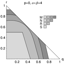
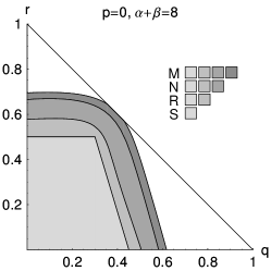
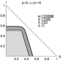
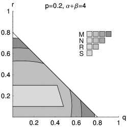
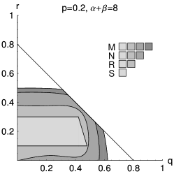
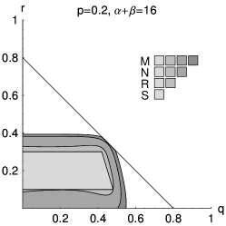
Figure 1: The sets of states (68) which fulfill the respective inequalities derived from transposition map (decomposition (49)) are shown in different tones of grey. The set labeled M contains all states that satisfy inequality (29), N– satisfy (32) with $\alpha\geq 1,\beta=1$, R - satisfy (32) with $\alpha=1,\beta\geq 1$, S - satisfy the positive partial transposition criterion. Parameter $\alpha+\beta$ corresponds to the sum of powers; in the case of inequality (29) we use the convention that $\beta=0$; parameter $p$ describes a considered class of states (see Eq. (68)). The triangle marked in the figure denotes the set of all states.

Let us first present the plots for inequalities of both types, i.e. of the form (29) and (32) for rotationally invariant states (68). In Figure 1 we compare the areas detected by the two inequalities arising from transposition map and taken with integer $\alpha\geq 1$. In Figure 2 the same is shown for the Breuer-Hall map (with $U=V$, where $V$ is a unitary antisymmetric matrix with the only nonzero entries $\pm 1$ lying on the anti–diagonal).

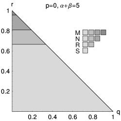
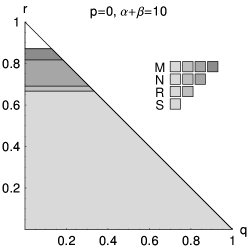
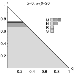
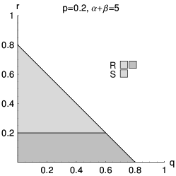
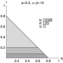
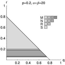
Figure 2: The sets of states (68) that fulfill the respective inequalities derived from the Breuer map [51] (i.e. the map (15) taken with $U$ being a unitary antisymmetric matrix with the only nonzero entries $\pm 1$ lying on the antidiagonal) using the decomposition (49)) are shown in different tones of gray. The set labeled M contains all states that satisfy inequality (29), N - satisfy (32) with $\alpha\geq 1,\beta=1$, R - satisfy (32) with $\alpha=1,\beta\geq 1$, S - satisfy the Breuer–Hall criterion. If the state is not explicitly marked it means that it is the same as the largest set in the picture. Parameter $\alpha+\beta$ corresponds to the sum of powers; in the case of inequality (29) we use the convention that $\beta=0$; parameter $p$ describes a considered class of states (see Eq. (68)). The triangle marked in the figure denotes the set of all states.

Only the decomposition (49), corresponding to maximal length of $\Lambda_{1}$, is considered since it leads to inequalities for entropies similar to standard ones.

As another example we show the effectiveness of inequalities derived from reduction map. We consider a class of isotropic states (69). In Figure 3, we show the percentage of entangled states detected by inequalities presented here as a function of the total power $\alpha+\beta$ (corresponding to number of copies in a multicopy measurement). The percent is taken with respect to all states detected by the reduction map, and the measure applied hear is the Euclidean measure on the parameter space. All the measures were determined numerically. Note that in this case inequality (32) taken with $\beta=1$ is a standard entropic inequality (5).

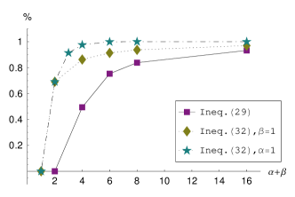
Figure 3: The percentage of the isotropic states (69) detected by the inequalities derived from reduction map (decomposition (49)) as a function of parameter $\alpha+\beta$ ($\alpha+\beta$ corresponds to the sum of powers); in case of inequality (29), $\beta=0$; parameter $p$ describes a considered class of states.

Both provided examples confirm that for states with maximally mixed subsystem and particular choice of $\alpha+\beta$, the largest set of entangled states is detected by inequality (32) with $\alpha=1$ (the strongest criterion for states with maximally mixed subsystem), and the smallest by inequality (29) (the weakest from the separability criteria derived here). Moreover, the larger the power $\alpha+\beta$, the more states detect both inequalities. Analysis of states which do not have a maximally mixed subsystems (see below) will show that this is not a general rule.

It was already mentioned that the effectiveness of inequalities depends strongly on the choice of decomposition of a map. Let us now present this effect for inequalities derived from transposition map and applied to rotationally invariant states (68) with $p=0$. The so–called minimal decomposition of the transposition map is given in Eq. (3.3). The completely positive maps $T_{1(2)}$ in Eq. (3.3) have the Kraus representation involving $SU(d)$ generators and identity. The map $T_{1}$ has minimal length $d(d+1)/2$ and $T_{2}$ has the minimal length $d(d-1)/2$. We obtain other decompositions of transposition map, with larger $\kappa_{1}$, by adding and subtracting the term $V_{i}\varrho V_{i}^{\dagger}$, which is in the Kraus representation of $T_{2}$ but not in the representation of $T_{1}$. In this way, the length of $\Lambda_{2}$ does not change (even though the map itself changed), and the length of $\Lambda_{1}$ is enlarged by one. Using this technique we got several different decompositions of the transposition map and checked how much entanglement in $4\otimes 4$ rotationally invariant states (68) with $p=0$ can be detected by the inequalities with the same $\alpha$ but different $\Lambda_{1}$ and $\Lambda_{2}$. The results for inequality (29) are presented in Figure 4a ($\kappa_{1}=16$ corresponds to decomposition from Table 2, while $\kappa_{1}=10$ to equation (3.3)). The percent of detected entangled states is taken with respect to the amount of states detected by the transposition map itself, and the measure used here is the Euclidean measure on the parameter space which was determined numerically. The trend, similar for all values of parameter $\alpha$, is such that the larger the length of $\Lambda_{1}$ the more entanglement detects the respective inequality. A similar analysis conducted for inequality (32) presented in part (i) of the Theorem 2 for $\alpha\neq 1,\beta=1$ reveals a similar trend. The dependence on decomposition is shown in Fig. 4b.

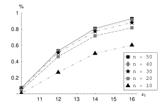
a) b)

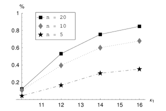
Figure 4: The percent of states (68) with $p=0$ detected by the inequalities as a function of length of map $\Lambda_{1}$ in various decompositions of the transposition map (described in the text). The plots were made for a) inequality (29) and b) inequality (32) with $\alpha>1,\beta=1$, $n=\alpha+\beta$. In each plot, on the vertical axis the scale is $0$ to $1$, where $1$ corresponds to $100\%$. The percent of states detected by the inequalities is taken with respect to the set of states detected by transposition map.

Let us now use the derived inequalities to analyze the separability of states (70), which do not have a maximally mixed subsystem, and are entangled for the whole range of parameters. We apply the inequalities derived from a few decompositions of the reduction criterion acting on subsystem $B$: firstly, the minimal decomposition, $\Theta_{1}^{(1)}(\varrho)=\varrho_{A}\otimes\mathbbm{1}_{d}-(1/2)\varrho$, $\Theta_{2}^{(1)}(\varrho)=(1/2)\varrho$, secondly, the decomposition with $\Lambda_{\Tr{}}$, $\Theta_{1}^{(2)}(\varrho)=\varrho_{A}\otimes\mathbbm{1}_{d}$, $\Theta_{2}^{(2)}(\varrho)=\varrho$, and thirdly, $\Theta_{1}^{(3)}(\varrho)=\varrho_{A}\otimes\mathbbm{1}_{d}+\varrho$, $\Theta_{2}^{(3)}(\varrho)=2\varrho$. Analogous decompositions are derived for the map acting on subsystem $A$. The results obtained are presented in Fig. 5 for the map acting on subsystem $A$, and in Fig. 6 for subsystem $B$. In both figures the percent of entangled states detected by various inequalities is plotted versus parameter $\alpha+\beta$. Interestingly, for this class of states, increasing the parameter $\alpha+\beta$ does not always lead to a stronger separability criterion. When the inequality (32) with $\alpha\geq 1,\beta=1$ is considered, the larger parameter $\alpha$ the less entangled states is detected (see, e.g. Fig. 5b). Moreover, one can again see how the choice of decomposition influences effectiveness. In all figures, the greatest amount of detected entangled states corresponds to decomposition (3), whereas the smallest amount to minimal decomposition (1). Inequality (32) taken with $\alpha=1,\beta\geq 1$ does not depend on decomposition in this case since $\Lambda_{2}$ changes only up to a constant. Moreover, it detects all states for all $\beta\geq 1$.

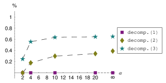
a)b)

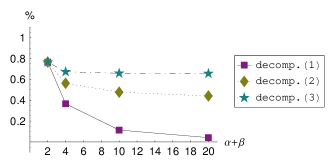
Figure 5: The percentage of states given by Eq. (70) detected by the inequalities derived from decompositions (1), (2) and (3) of the reduction map (defined in the text above the figure as $\Theta_{i}^{(1)}$, $\Theta_{i}^{(2)}$ and $\Theta_{i}^{(3)}$) acting on subsystem $A$, as a function of $\alpha$ or $\alpha+\beta$. The plots were made for a) inequality (29) and b) inequality (32) with $\alpha>1,\beta=1$. In each plot, on the vertical axis the scale is $0$ to $1$, where $1$ corresponds to $100\%$. The percentage is taken with respect to all states (all entangled states are detected by reduction map).

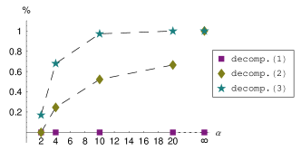
a)b)

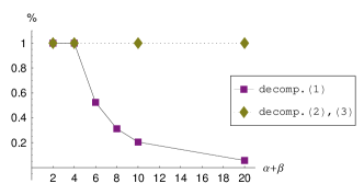
Figure 6: The percent of states given by Eq. (70) detected by the inequalities derived from various decompositions of the reduction map (described in the text) acting on subsystem $B$, versus parameters $\alpha$ and $\alpha+\beta$. The plots were made for a) inequality (29), b) inequality (32) with $\alpha>1,\beta=1$. In each plot, on the vertical axis the scale is $0$ to $1$, where $1$ corresponds to $100\%$. The percent is taken with respect to all states (all states are detected by reduction map).

5 Conclusion

To summarize, firstly, we have presented a simple generalization of the Nielsen–Kempe disorder criterion to any possible positive map $\Lambda:M_{d}(\mathbb{C})\to M_{d}(\mathbb{C})$. However, the cost we have to pay for this generality is that instead of majorization we have to use the notion of weak majorization, losing such a clear physical interpretation as in the case of majorization relations. Furthermore, our relations do not reproduce the Nielsen–Kempe result when the reduction map is considered. They only give equivalent criterion for states with at least one maximally mixed subsystem. On the other hand, taking other positive maps and in particular indecomposable ones, we can obtain stronger separability criteria.

Still, the open question remains about possibility of derivation of majorization relations (not weak majorization) from any positive map, not only the reduction one. One of the possible ways is the following. Assume that $[I\otimes\Lambda](\varrho)\geq 0$ with $\Lambda$ being some positive map for which equation (51) holds. Then rewrite the latter as

$$\varrho_{A}\otimes\mathbbm{1}_{d}\geq\frac{\eta_{d}}{\xi}[I\otimes\Phi](\varrho).$$ (71)

Note that for the best known positive maps (see Table 2) the above decomposition holds and $\eta_{d}\geq\xi$, which allows us to write

$$\varrho_{A}\otimes\mathbbm{1}_{d}\geq[I\otimes\Phi](\varrho).$$ (72)

Note, however, that above formula is a reduction criterion for the state $[I\otimes\Phi](\varrho)$, which due to [37] leads straightforwardly to $\lambda(\varrho_{A})\succ\lambda([I\otimes\Phi](\varrho))$. This relation, however, may be directly obtained from the Nielsen–Kempe majorization criterion, as for any quantum channel and separable state $[I\otimes\Phi](\varrho)$ is also separable state and must obey this criterion.

Secondly, we have provided two methods of deriving some entropic–like or entropic inequalities. The big advantage of the present approach is that, contrary to the method of [39, 40], the present method does not require any assumptions about the investigated state, i.e. works for any bipartite state. The first of proposed method bases on the weak majorization criteria. To derive the second class of entropic inequalities, we utilized some class of functional inequalities. This is a continuation and extension of the results presented in [40] where we have provided some inequalities stronger than the standard entropic inequalities and allowing for the detection of bound entanglement.

Moreover, it is pointed out that both the weak majorization criterion, and the inequalities derived from decomposition (49) of some map $\Lambda$ lead, for states with at least one maximally mixed subsystem, to the criterion equivalent to the necessary criterion $[I\otimes\Lambda](\varrho)\geq 0$.

The derived generalizations of entropic inequalities were analyzed in the context of the protocol of state merging and approximation of a mean value of a linear entanglement witness. Moreover, all the derived inequalities (with integer $\alpha$ and $\beta$) contain expressions involving products of operators, e.g. $\Tr[I\otimes\Lambda_{1}(\varrho)]^{\alpha}[I\otimes\Lambda_{2}(\varrho)]^{\beta}$, which can be (in principle) measured experimentally as a mean value of some operator (multi–copy entanglement witness) on a number of copies of a state. In the case of the first method (e.g. inequalities (29), the number of copies is equal to $\alpha$, while in the case of inequalities (32), one has to take $\alpha+\beta$ copies of a given state at a time. A detailed analysis of this approach can be found in [33, 39].

6 Acknowledgments

We gratefully acknowledge M. Horodecki and M. Lewenstein for discussions. This work was prepared under the support of EU IP SCALA. R.A. gratefully acknowledges the support from the Foundation for Polish Science and MEC (Spain) under the program Consolider-Ingenio 2010 QOIT. J.S. acknowledges financial support from MCI (Spain) under the contract FIS2008-01236/FIS and the ‘Universitat Autònoma de Barcelona’.

References

References

- [1] R. Horodecki, P. Horodecki, M. Horodecki, K. Horodecki, Rev. Mod. Phys. 81, 865 (2009).
- [2] R. F. Werner, Phys. Rev. A 40, 4277 (1989).
- [3] A. Peres, Phys. Rev. Lett. 77, 1413 (1996).
- [4] R. Horodecki, M. Horodecki, and P. Horodecki, Phys. Lett. A 210, 227 (1996).
- [5] M. Horodecki, P. Horodecki, and R. Horodecki, Phys. Lett. A 223, 1 (1996).
- [6] P. Horodecki, Phys. Lett. A 232, 333 (1997).
- [7] M. A. Nielsen and J. Kempe, Phys. Rev. Lett. 86, 5148 (2001).
- [8] J. K. Korbicz, J. I. Cirac, and M. Lewenstein, Phys. Rev. Lett. 95, 120502 (2005); Phys. Rev. Lett. 95, 259901 (2005).
- [9] J. K. Korbicz, O. Gühne, M. Lewenstein, H. Häffner, C. F. Roos, and R. Blatt, Phys. Rev. A 74, 052319 (2006).
- [10] O. Gühne and N. Lütkenhaus, Phys. Rev. Lett. 96, 170502 (2006).
- [11] J. de Vicente, Quantum Inf. Comput. 7, 624 (2007).
- [12] C.–J. Zhang, Y.-S. Zhang, S. Zhang, G.-C. Guo, Phys. Rev. A 77, 060301(R) (2008).
- [13] O. Gühne, P. Hyllus, O. Gittsovich, J. Eisert, Phys. Rev. Lett. 99, 130504 (2007).
- [14] J. Sperling and W. Vogel, Phys. Rev. A 79, 022318 (2009).
- [15] G. Tóth, C. Knapp, O. Gühne, and H. J. Briegel, Phys. Rev. Lett. 99, 250405 (2007); G. Tóth, C. Knapp, O. Gühne, and H. J. Briegel, Phys. Rev. A. 79, 042334 (2009).
- [16] O. Gühne and G. Tóth, Phys. Rep. 474, 1 (2009).
- [17] S. P. Walborn, P. H. Souto Ribeiro, L. Davidovich, F. Mintert, and A. Buchleitner, Nature 440, 1022 (2006); L. Aolita and F. Mintert, Phys. Rev. Lett. 97, 050501 (2006).
- [18] R. Augusiak, M. Demianowicz, and P. Horodecki, Phys. Rev. A 77, 030301(R) (2008).
- [19] M. Horodecki and P. Horodecki, Phys. Rev. A 59, 4206 (1999).
- [20] N. J. Cerf, C. Adami, and R. M. Gingrich, Phys. Rev. A 60, 898 (1999).
- [21] P. Horodecki and A. Ekert, Phys. Rev. Lett. 89, 127902 (2002); P. Horodecki, Phys. Rev. Lett. 90, 167901 (2003); H. A. Carteret, Phys. Rev. Lett. 94, 040502 (2005); P. Horodecki, R. Augusiak, and M. Demianowicz, Phys. Rev. A 74, 052323 (2006).
- [22] R. Horodecki and P. Horodecki, Phys. Lett. A 194, 147 (1994).
- [23] M. Horodecki, J. Oppenheim, A. Winter, Nature 436, 673 (2005); M. Horodecki, J. Oppenheim, A. Winter, Commun. Math. Phys. 269, 107 (2007).
- [24] R. Horodecki and M. Horodecki, Phys. Rev. A 54, 1838 (1996).
- [25] B. M. Terhal, Theor. Comput. Sci. 287, 313 (2002).
- [26] K. G. H. Vollbrecht and M. Wolf, J. Math. Phys. 43, 4299 (2002).
- [27] A. Rényi, Proc. Fourth Berkeley Symp. on Math. Statist. and Prob., Vol. 1 (Univ. of Calif. Press, 1961).
- [28] C. Tsallis, J. Stat. Phys. 52, 479 (1988).
- [29] A. Wehrl, Rev. Mod. Phys. 50, 221 (1978).
- [30] S. Abe and A. K. Rajagopal, Physica A 289, 157 (2001); C. Tsallis, S. Lloyd, and M. Baranger, Phys. Rev. A 63, 042104 (2001); J. Batle, M. Casas, A. Plastino, and A. R. Plastino, ibid. 71, 024301 (2005), and references therein.
- [31] K. Życzkowski, P. Horodecki, M. Horodecki, R. Horodecki, Phys. Rev. A 65 012101 (2002).
- [32] R. Rossignoli and N. Canosa, Phys. Rev. A 66, 042306 (2002); R. Rossignoli and N. Canosa, ibid. 67, 042302 (2003).
- [33] P. Horodecki, Phys. Rev. A 68, 052101 (2003).
- [34] F. A. Bovino, G. Castagnoli, A. Ekert, P. Horodecki, C. Moura Alves, and A. V. Sergienko, Phys. Rev. Lett. 95, 240407 (2005).
- [35] Ch. Schmid, N. Kiesel, W. Wieczorek, H. Weinfurter, F. Mintert, and A. Buchleitner, Phys. Rev. Lett. 101, 260505 (2008).
- [36] C. Moura Alves and D. Jaksch, Phys. Rev. Lett 93, 110501 (2004).
- [37] T. Hiroshima, Phys. Rev. Lett. 91, 057902 (2003).
- [38] M. Horodecki, P. Horodecki, and R. Horodecki, Phys. Rev. Lett. 80, 5239 (1998).
- [39] R. Augusiak, J. Stasińska, and P. Horodecki, Phys. Rev. A 77, 012333 (2008).
- [40] R. Augusiak and J. Stasińska, Phys. Rev. A 77, 010303(R) (2008).
- [41] P. M. Alberti and A. Uhlmann, Stochasticity and Partial Order—Doubly Stochastic Maps and Unitary Mixing, Mathematics and its Applications vol. 9 (D.Reidel Publ. Company, Dordrecht, 1982).
- [42] M. A. Nielsen, Phys. Rev. Lett. 83, 436 (1999).
- [43] M. A. Nielsen and G. Vidal, Quantum Inf. Comput. 1, 76 (2001).
- [44] R. Bhatia, Matrix Analysis (Springer, New York, 1997).
- [45] A. W. Marshall and I Olkin, Inequalities: Theory of Majorization and Its Applications, Mathematics in Sciences and Engineering Vol. 143, (Academic Press, New York, New York, 1979).
- [46] A. Jamiołkowski, Rep. Math. Phys. 3, 275 (1972).
- [47] M.-D. Choi, Linear Alg. Appl. 10, 285 (1975).
- [48] J.-C. Hou, J. Oper. Theory 39, 43 (1998).
- [49] K. Kraus, States, Effects and Operations: Fundamental Notions of Quantum Theory, (Wiley, New York, 1991).
- [50] A. Jamiołkowski, Open Sys. and Inf. Dyn. 11, 385-390 (2004).
- [51] H.–P. Breuer, Phys. Rev. Lett. 97, 080501 (2006).
- [52] W. Hall, J. Phys. A: Math. Theor. 40, 6183 (2007).
- [53] S. Arimoto, Inf. Control 19, 181 (1971).
- [54] K. Löwner, Math. Z. 38, 177 (1934).
- [55] G. Lindblad, Commun. Math. Phys. 28, 245 (1972).
- [56] R. F. Werner, A. S. Holevo, J. Math. Phys. 43, 4353 (2002).
- [57] M.-D. Choi, Linear Algebr. Appl. 12, 95 (1975).
- [58] K. Tanahasi and J. Tomiyama, Can. Math. Bull. 31, 308 (1988); H. Osaka, Linear Algebr. Appl. 153, 73 (1991); H. Osaka ibid 186, 45 (1993).
- [59] K.-C. Ha, Publ. Res. Inst. Math. Sci. 34, 591 (1998).
- [60] J. Schliemann, Phys. Rev. A 68 , 012309 (2003).
- [61] J. Schliemann, Phys. Rev. A 72, 012307 (2005).
- [62] H.–P. Breuer, Phys. Rev. A 71, 062330 (2005).
- [63] H.–P. Breuer, J. Phys. A 38, 9019 (2005).
- [64] R. Horodecki, Phys. Lett. A 210, 223 (1996).