Quantitative Measurements of CME-driven Shocks from LASCO Observations

Abstract

In this paper, we demonstrate that CME-driven shocks can be detected in white light coronagraph images and in which properties such as the density compression ratio and shock direction can be measured. Also, their propagation direction can be deduced via simple modeling. We focused on CMEs during the ascending phase of solar cycle 23 when the large-scale morphology of the corona was simple. We selected events which were good candidates to drive a shock due to their high speeds (V$>$1500 km s^-1). The final list includes 15 CMEs. For each event, we calibrated the LASCO data, constructed excess mass images and searched for indications of faint and relatively sharp fronts ahead of the bright CME front. We found such signatures in 86% (13/15) of the events and measured the upstream/downstream densities to estimate the shock strength. Our values are in agreement with theoretical expectations and show good correlations with the CME kinetic energy and momentum. Finally, we used a simple forward modeling technique to estimate the 3D shape and orientation of the white light shock features. We found excellent agreement with the observed density profiles and the locations of the CME source regions. Our results strongly suggest that the observed brightness enhancements result from density enhancements due to a bow-shock structure driven by the CME.

1 Introduction

Coronal Mass Ejections (CMEs) are the largest transient expulsions of coronal material in the heliosphere. These explosive events are recorded by coronagraphs as brightness enhancements in white light images because the ejected material scatters a large amount of photospheric light. In image sequences, local brightness changes provide most of the information on CME parameters, such as speed and mass. LASCO (Brueckner et al., 1995) observations have established that CME speeds vary from a few hundred to more than 2500 km/s (Yashiro et al., 2004). With this wide range, it is reasonable to expect that CME speeds often exceed the local magnetosonic speed, and drive a shock wave in the low corona (Hundhausen, 1987).

There are two main observational results that provide support for the existence of shocks in the low corona. Metric type-II radio bursts provide indirect evidence of CME-driven shocks (e.g., Cliver et al., 1999), but the scarcity of imaging radio observations precludes the reliable identification of the driver. Observations of distant (from the CME) streamer deflections (e.g., Gosling et al., 1974; Michels et al., 1984; Sheeley et al., 2000) provide the most reliable indication of a CME-driven wave pushing out the streamers. However, there remains the question of whether this wave is a shock wave, specially for the cases where the CME speed is not excessively high. Vourlidas et al. (2003) presented the first direct detection of a CME-driven shock in white light images, combining two signatures: (1) a sharp but faint brightness enhancement ahead of the CME and (2) a streamer deflection well-connected to the expansion of the sharp front. Vourlidas et al. (2003) confirmed that the white light signature was a shock wave using an MHD simulation based on the measured CME speed and location.

Despite the large number of CME observations with LASCO, CME-driven shocks in white light images remain difficult to detect. The brightness enhancement due to the shock itself is faint and can be easily lost in the background corona which changes from event to event. Projection effects can also make it difficult to recognize and separate the shock signatures from the rest of the CME because deflected streamers, the shock and the CME material can all overlap along a given line of sight (LOS). If the shock exists, however, it will result in a density enhancement and, with proper analysis, should be visible in the images.

We note that the earlier paper by Vourlidas et al. (2003) discussed shock signatures related to rather small and fast events (such as surges and jets). Here we extend the detection of white light signatures to standard CMEs by analyzing a set of fast CMEs during the rising phase of solar cycle 23. These two papers suggest that white light shock signatures must be a common feature in coronagraph images and the previous scarcity of shock detections is mostly due to reduced sensitivity, fields of view and temporal coverage of past instruments.

The data selection and methodology are described in § 2. The unique aspects of this work are the quantitative density measurements that allow us to estimate the shock strength, as presented in § 3, and the analysis of the 3D morphology and orientation of the white light shock using the Solar Corona Raytrace (SCR), a software package that simulates the appearance of various 3D geometries in white light coronagraph images (Thernisien et al., 2006). We compare the modeled images to density profiles obtained from LASCO images in § 4 and found them in excellent agreement. A summary and general discussion are presented in § 5.

2 Event Selection and Identification of the White Light Shock

To identify a sample of CME events with likely shock signatures, we used two general criteria: (1) we searched for fast CMEs ($>$1500 km s^-1) because they are more likely to drive a shock, and (2) we considered only CMEs occurring at the ascending phase of the solar cycle 23 (1997-1999), when the simple morphology of the background white light corona offers a better chance to observe faint shock-like structures with minimal confusion from overlapping structures along the LOS. Only 15 CMEs (out of about 2000) satisfied our selection criteria and are shown in Table 1. The first and second column are the number and the date of the event; the third column is the time of first appearance in LASCO C2; the fourth, fifth and sixth columns are the linear speed, angular width (AW) and the central position angle (PA) respectively, as reported in the CME LASCO catalog (Yashiro et al., 2004). The seventh column shows whether the CME is associated with a decimetric type II radio burst (Gopalswamy et al., 2005).

To identify whether a shock signature exists in a given LASCO image, we look for white light features that satisfy the following criteria: (1) it must be a smooth, large scale front, (2) it must outline the outermost envelope of the CME, and (3) it should be associated, spatially and temporally, with streamer deflections. We choose these criteria based on our expectations of how a CME-driven shock should behave; namely, it should be ahead of the CME material (the driver), it should expand away from the CME over large coronal volumes (but avoiding coronal holes, for example), and it should affect streamers when it impinges on them (Vourlidas et al., 2003).

It turns out that such fronts exist in the majority of the images we looked at but they are generally much fainter than most of the other CME structures. They remain unnoticed in the running difference or quick-look LASCO images normally published in the literature. These fronts become visible only when the brightness scale of these images is saturated to bring out the fainter structures.

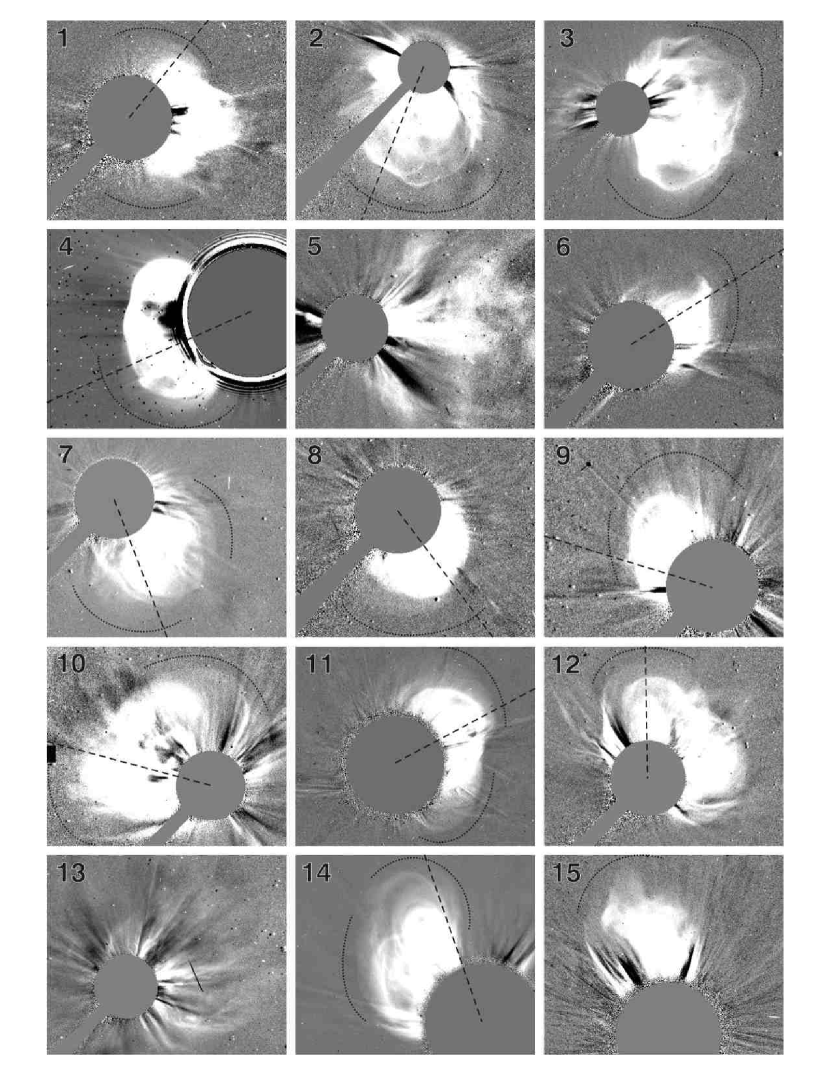
Figure 1: The sample of the 15 fastest CMEs observed by the LASCO coronagraphs between 1997 and 1999. The image with the clearest shock signature is shown in each panel. The radial lines mark the position angles of the density profiles analyzed. The curved lines are visual guides for the location and extent of the faint shock structures. These features may be more visible in the online version of the figure. For events 5 and 13 it was not possible to determine a clear signature due to the disturbed background corona.

We are able to identify and analyze these fronts because we use calibrated LASCO images. The calibration brings out faint structures, which may be missed in standard image processing, because it removes vignetting and other instrumental effects. We use excess mass images from both LASCO C2 and C3. These are calibrated images from which a pre-event has been subtracted thus removing the background corona (Vourlidas et al., 2000). A frame from each of our CMEs is shown in figure 1. Most of the images have a curved line to guide the reader’s eye to the shock signature, while the dashed line in each frame is pointing out the position angle corresponding to the measurements that will be explained in section § 3.3. Because of the large variation in the brightness of the features, we have to apply different contrasts to bring out the shock signature in each CME. In most images, the shock signature is associated with diffuse emission on the periphery of the much brighter CME material. The diffuse emission could arise from the coronal material on the shock surface. For some events, like #1, #6, or #11, the faint emission encompasses the CME as one would expect for an ideal case of a shock enveloping the driver. In other events, e.g #8, #9 and #12, the faint emission is only seen over a small range of position angles. In all cases, the emission has a smooth front, follows the general shape of the driver material (the bright CME core), and is associated with a streamer bent from its pre-event position. All these features are clear indications that we are dealing with a wave.

The reason why we are confident that what we observe is indeed a shock wave lies with the CME speed. All our events are either halo or partial halo CMEs, and their speeds are lower limits to the true speeds. Even these lower limit speeds are sufficiently high to create a shock wave for typical values of plasma parameters in the low corona (Hundhausen, 1987). Therefore, we will refer to the observed feature as shocks, from now on.

3 Shock Measurements

3.1 Shock Signature Evaluation

We identified a shock signature in the LASCO images for 13 out of the 15 selected events. For events #5 and #13, it was not possible to find a feature that satisfied even one of our three selection criteria (§ 2). We believe that the lack of a smooth front and streamer deflections may be due to the presence of a previous CME. In both cases, the excess mass images showed clear evidence of a disturbed corona (e.g., mass depletions, streamer displacements). A shock may not form if the first event has altered the background magnetic field considerably. Even if it forms, as the DM Type-II emissions suggest, it is unlikely to develop a smooth, large front as it propagates through such a disturbed medium. Similarly for streamer deflections, many of the streamers could have already been deflected by the previous CME at various angles from the sky plane and any new deflection may not register as a smooth front in the images. Finally, the strong intensity variations left on the image by the previous CME may mask any faint fronts associated with the shocks from our CMEs. It seems, therefore, that a relatively unperturbed corona facilitates the detection of the faint CME-driven shocks. Nevertheless, once we establish which signatures are shock-related, we expect it will become easier to analyze events in more disturbed coronal conditions.

For events #4, #10 and #11, we found a clear shock signature in the LASCO C2 images, while for the rest of the events, the clearest signatures were found in the LASCO C3 images. We found at least one location with a clear white light shock signature for all halo CMEs (10 events). This is expected if our shock interpretation is correct since halos offer the best viewing of the CME flanks due to their propagation along the LOS. We also note that our interpretation implies that a major part of the halo CME extent is due to the shock rather than actual ejected material and analysis of CME widths need to take this fact into consideration.

3.2 From Mass Profiles to Density Ratios

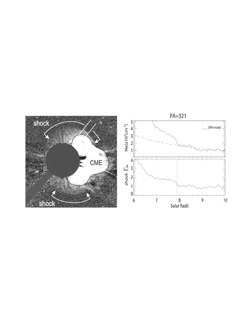
Figure 2: Left panel: Selected image for the November 6, 1997 CME. A clear shock signature can be seen at the flanks of the CME. The parallel lines over the shock front show the profile with the strongest shock signature. Right panel: The top plot shows the estimated up-stream and down-stream density profile at PA = 312 (solid) and the background corona density from the SPM model (dashed). The bottom plot shows the density ratio, $\Gamma_{CR}=1.6$, at $7.9$ $R_{\sun}$ which we use as a proxy to the shock strength.

We can use the calibrated LASCO images not only to identify the faint shock fronts but also to derive some estimates of the density profile across these fronts. Each pixel in the mass LASCO images gives the total mass or, equivalently, the total number of electrons along the LOS. This excess electron column density (e/cm²) can be converted to electron volume density (e/cm³), if the depth of the structure along the LOS is known. This quantity is unknown and it cannot be reliably estimated without some knowledge of the 3D morphology of the structure. We address the 3D aspect in § 4 but for the analysis we assume a nominal depth of 1 R_☉ for all the events because it is a convenient scale and likely a good upper limit given the slope ($\sim 0.3R_{\sun}$) of the brightness profiles (e.g., figure 2).

We then derive the total electron column density along the profile, by integrating the density of the background equatorial corona from the Saito, Poland, Munro (SPM) model (Saito et al., 1977). Again, the actual value of the background density for each event is not known and we have to resort to a density model as is often the case in analysis of coronal observations. Here we assume that the same equatorial SPM model applies to all events for two reasons: (1) our sample covers only a small phase of the solar cycle when the average density of the background corona does not vary significantly, and (2) the density enhancement at the shock front must come from streamer material since shocks do not propagate, nor pile up material over coronal holes.

3.3 Estimation of the Shock Strength

For each event we chose the image with the visually clearest shock signature. In that image, we obtain several profiles at different PAs along the shock front. Our method averages the emission along a narrow range of PAs ($\sim$5$\arcdeg$) to improve the signal-to-noise ratio. The radial extent of each profile allows us to obtain the upstream and downstream brightness at different angles of the shock (see also Vourlidas et al., 2003) and convert them to densities as mentioned in § 3.2. We classify the 15 events in four groups based on the appearance of the shock signatures in the images and the evidence of a jump in the density profiles. Group 1 includes those events which have a clear shock signature in the image and a steep jump in the brightness profiles at the location of the shock front (6 events). Group 2 includes those events which show a clear shock signature in the image but the density jump at the shock front is barely detectable above the noise (5 events). Group 3 includes those events which have shock signatures in the image but the density profiles are too noisy to identify the jump at the shock front; there were 2 events in Group 3. Finally, Group 4 are the two events (#5 and #13) without any shock signatures in any LASCO image.

The shock fronts are more visible on the images rather than in the density profiles because of our eyes’ spatial averaging ability. We believe that the density profiles can be improved by averaging over a larger angular width. However, this averaging tends to smooth the profiles and reduce the density jump. Until we find a better averaging method we adopted the $5\arcdeg$ width in the current work.

For this reason, we concentrate on the profiles with the sharpest density jump. We use the density jump as a proxy to the shock strength. We define $\Gamma_{CR}$ as the compression ratio of the total to background volume densities, $\Gamma_{CR}=1+\frac{\rho}{\rho_{0}},$ where $\rho$ is the excess density due to the shock, and $\rho_{0}$ the upstream density obtained from the SPM model.

Figure 2 shows event #1 as an example. The two parallel lines mark the position angles we average over to obtain the brightness profile with the sharpest density jump, and hence the strongest shock signature. The jump is located at 7.9 R_☉ at PA$=$321$\arcdeg$. The observed density profiles and the ratio between excess and background densities are plotted on the right panels of figure 2. In this case, we obtain a $\Gamma_{CR}$ of 1.6 at the location of the shock. We repeat the same analysis for the remaining events in our sample. We also obtain the CME mass, momentum and kinetic energy from the same images following the method described by Vourlidas et al. (2000) and using the speed measurements from the LASCO CME catalog. These measurements allow us to get global CME parameters to compare with the local shock strength, which are discussed next.

3.4 Statistics

Table 2 presents our measurements for the 13 events. Columns 1-2 correspond to the event number (1) and its group ( §3.1). Columns 3 to 6 are the time of LASCO observation, the heliocentric distance to the shock signature, the PA of the profile and the estimated density jump, $\Gamma_{CR}$, of the shock for that profile. Columns 7 to 9 are the CME mass, kinetic energy and momentum respectively, obtained from calibrated images. Now we can assess the validity of our main assumption; namely, whether the faint structures seen ahead of the main CME ejecta could indeed be the white light counterpart of the CME-driven shock. If this is true, we expect a correlation between the magnitude of the density jump (or $\Gamma_{CR}$) and the CME dynamical parameters, such as the CME kinetic energy.

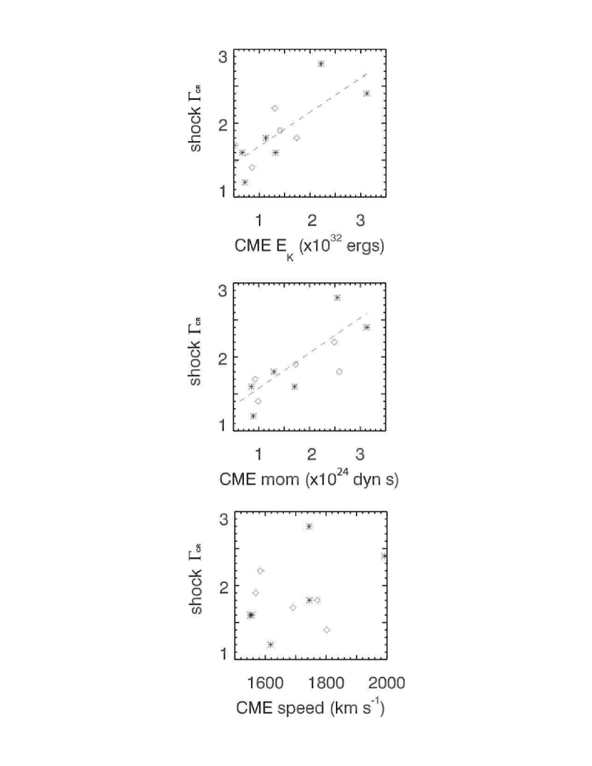
Figure 3: Trends and correlations between estimated shock $\Gamma_{CR}$ and select CME parameters. The top and middle panels show the correlations between the shock $\Gamma_{CR}$ and the CME kinetic energy (cc=0.77) and momentum (cc=0.80), respectively. The bottom panel shows no clear correlation between the shock $\Gamma_{CR}$ and the CME speed (group 1: stars, group 2: diamonds).

The plots in figure 3 show the trends and correlations obtained between $\Gamma_{CR}$ and some CME parameters for the best events only (groups 1 and 2). We find important correlations between the shock strength and the CME momentum (cc=0.80), and kinetic energy (cc=0.77). Furthermore, the largest $\Gamma_{CR}$ are associated with the sharpest shock signatures (group 1, see § 3.1) and the highest kinetic energies and momenta. These results suggest that our $\Gamma_{CR}$ parameter is associated with the CME dynamics as expected from a shock-produced density jump.

Perhaps surprisingly, there is no obvious correlation between the strength and the linear speed of the CMEs. The quoted speeds are taken from the LASCO catalog and therefore correspond to the speed at the position angle of the fastest moving feature in the LASCO images. Our profiles were taken at different position angles since the shock front is more easily discernible at some distance away from the CME front. Also, the speeds are derived from linear fits to height-time measurements extending over the full range of the LASCO field of view (2-30 R_☉) and correspond to the average CME speed over the field of view. Our density jump is derived from a single snapshot of the CME at a single heliocentric distance. A plot between $\Gamma_{CR}$ and the CME speed at the same PA and distance might provide a better correlation. We tried to make these speed measurements. However, the large CME speed and synoptic LASCO cadences did not allow us to obtain a sufficient number of data points to derive reliable speed estimations for any of our events.

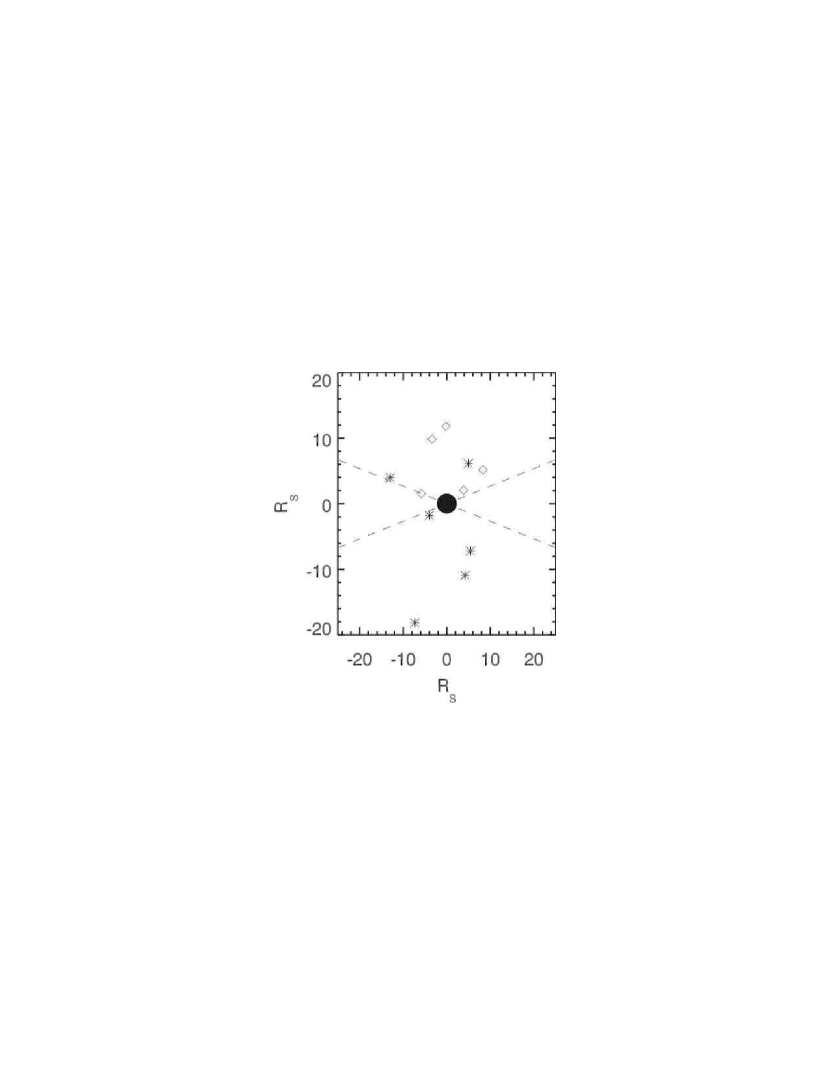
Figure 4: Locations on the plane of the sky of the clearest shock signatures in our event list. The dashed lines separate favorable and non-favorable position angles for a shock observation. All events showing a clear shock signature in the image and/or in the data analysis (stars and diamonds labels), are found below or above 15 degrees from the solar equator.

Figure 4 is related to the visibility of the shock signature in the LASCO images and shows that the clearest shock signatures were found above or below $15\arcdeg$ with respect to the solar equator. This holds even for the halo CMEs where there the shock is visible over more position angles. Considering the phase of the solar cycle, these results show that locations away from the streamers are favorable angles for shock signature observations on white light images. This result should be kept in mind when searching for shock signatures in coronagraph images. The complexity of the background corona masks the faint shock emissions during solar maximum while there are few sufficiently fast events to drive a shock during solar minimum.

4 Estimating the Shock Geometry with a Forward-Modeling Technique

The results in the previous sections provide ample support for a shock interpretation of the faint emission ahead of the CME front. In addition, we have devised a practical way to model the faint emission with a prescribed shape using forward modeling techniques. The advantages of this approach are the speed and simplicity of the software, and the resulting information on the 3D morphology and direction of the shock. The disadvantage is that we have no way of calculating a goodness of fit for the model other than a visual judgment on whether the envelope of the model fits the observed emission envelope. For the sake of brevity, we use the term ’fitting’ from now on to describe the ’fitting-by-eye’ we actually employed.

For simplicity, we assume that the CME-driven shock has a 3-D bow shock morphology, as expected from a body moving in uniform magnetized flow (e.g., Earth’s magnetosphere). We first need a geometric description for such a model. We found one in Smith, Khanzadyan, and Davis (2003) which is used to describe the shocks around Herbig-Haro objects. It is a a surface of revolution, in cylindrical coordinates and is described by the form (Eq. (1) in Smith, Khanzadyan, and Davis (2003))

$$\frac{z}{d}=\frac{1}{s}(\frac{R}{d})^{s}$$ (1)

where s controls the opening angle of the bow, d is a scale length (semilatus rectum) and $R$ is the heliocentric distance of the nose of the shock. The variables $d$ and $s$ control the shape of the bow shock and are the most important variables for visually matching the shock shape to the observations. To adopt this model for coronagraphic observations, we add a narrow shell of constant density, $N_{e0}$, and width, $\Delta$. In this way, we can calculate the brightness of the model using the Thomson scattering equations and the spacecraft geometry and analyze the model images exactly as we do the observations. We justify this shell as the plasma enhancement around the shock surface at a given moment. While plasma pileup at CME fronts is still an open question (Howard and Vourlidas, 2005), it is expected that the shock will cause local density enhancements as it propagates through the corona Vourlidas et al. (2003).

We use the SCR software package to create a simulated coronagraph image from the model. SCR is a numerical implementation of Thomson scattering that renders a total (or polarized) brightness 2D image as seen by a coronagraph (e.g. LASCO C2 or C3) given a 3D density structure distribution (Thernisien et al., 2006) and is available in Solarsoft. For all events, we assumed a constant thickness of $\Delta=0.3R_{\sun}$ which is comparable to the width of the brightness jump in the images. Because the height of the shock varied for each event, we set the density, $N_{e0}$ within the thin shell to the estimated density just ahead of the shock front (§ 3.2). Once the width and density of the model shock were set, we tried to match it to the LASCO images by varying its orientation in space and the geometric parameters of the parabola ($d$ and $s$). When we were satisfied that the simulated image fit visually the observed envelope of the shock, we integrated along the 3D shape, using the LASCO viewing geometry, and obtained a simulated brightness image of the model shock.

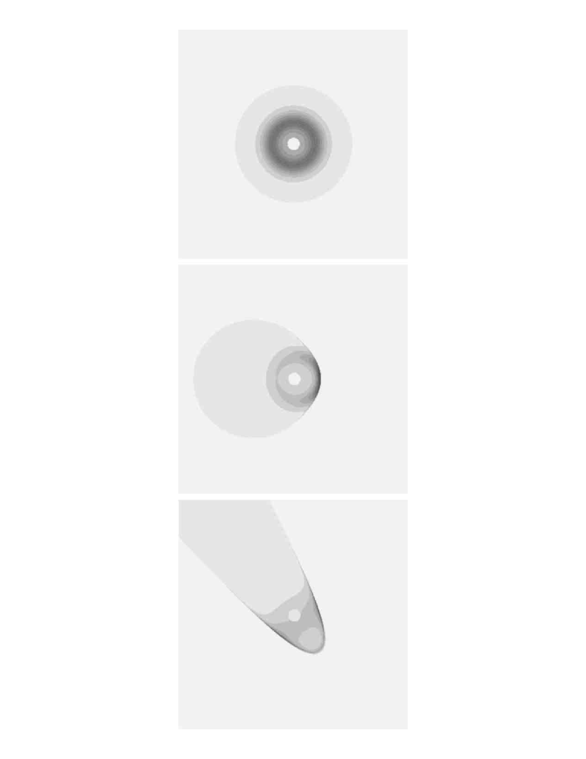
Figure 5: Simulated white light images for a bow-shock model at 8 R_☉ observed through different lines of sight, from top to bottom:(1) Along the Sun-Earth line, (2) 10$\arcdeg$ west and (3) 45$\arcdeg$ west, 45$\arcdeg$ south. The hole in the center of the images shows the size of the solar disk for scale. The intensity gradient represents the white light brightness of the model as viewed by LASCO C3.

Figure 5 shows simulated white light images of our bow-shock model viewed from different lines of sight: (1) Along the Sun-Earth line, (2) $10\arcdeg$ west and (3) 45$\arcdeg$ west, 45$\arcdeg$ south. The location of the bow shock nose is at 8 $R_{\sun}$. The images show the full model for completeness but we have restricted our integrations to a volume of $30R_{\sun}^{3}$, so the actual model is truncated and the long thin extensions in Figure 5 do not appear in our images.

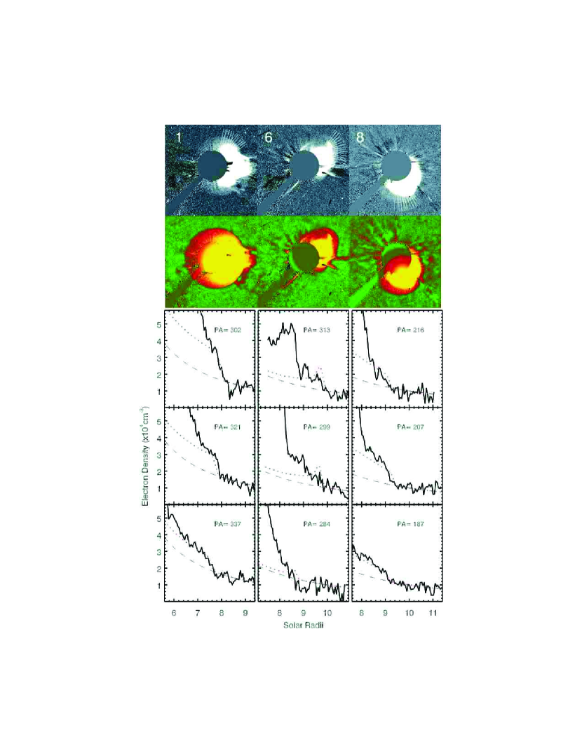
Figure 6: Comparing observed and modeled density profiles for events #1,# 6 and #8. From top to bottom for each column:(1) the actual LASCO image and the selected angles for obtaining the density profiles; (2) A synthetic coronagraph image of the shock model overplotted on the LASCO image; (3-5) comparison of density profiles at different PAs (solid line: LASCO density profile; dotted line: model shock density profile; dashed line: background coronal density from the SPM model).

To check whether the LASCO density profiles are consistent with a bow-shock geometry, we fit an SCR model to each event and obtained simulated density profiles over several PAs, using the same method as described in § 3.2 for the LASCO observations. This procedure is currently done by hand and the LOS integration is time-consuming in our hardware. We are working on improving it but so far we were able to perform detailed comparisons for only three events in our sample. We chose events #1 (November 6, 1997), #6 (June 4, 1998) and #8 (November 26, 1998), which have some of the clearest shock signatures. Figure 6 shows the results. Each plot shows the comparison between the SCR profiles to the LASCO ones for different PAs at the shock signature.

Figure 6 shows that the observed density profiles are consistent with a bow shock geometry for at least 30$\arcdeg$ along the shock signature. The density fits are surprisingly good given the simplicity of our model. Note that we did not attempt to fit either the density jump or the shock LOS extent. They were kept constant for each event. This result offers a strong indication that the overall envelope of enhanced emission around the CME must come from a simple structure (e.g., a bow shock) probably reflecting the simplicity of the minimum corona. In other words, the shock structure, and probably its visibility, may depend on the overall configuration of the large scale corona. It will be interesting to repeat our analysis for CMEs during the solar maximum.

Another consistency check comes from comparing the orientation of the bow shock shell in 3D space (which we get from the SCR modeling) to the expected orientation of the CME. For this, we make the usual assumption that the core of the CME (the driver for us) propagates radially outwards from the nearest possible source region (e.g., a flaring active region). The source regions for our three events are as follows:

• Event #1 is associated with the flare observed at 11:49 at S18W63. We took this location as the source region of the CME. Since this is a front side event, it is relatively easy to determine that there is no other active region with a better association.

• The LASCO movies suggest that event #6 is likely associated with a filament eruption on the far side of the Sun. The filament was seen for several days in H$\alpha$ images as it crossed over the western limb. Extrapolating from its known position on May 29th we estimate that the center of the filament would be at N43W107 on the day of the eruption.

• Event #8 is also a backside CME resulting in an indirect source region identification. We examined the EIT and LASCO movies for a few days before and during the eruption. The low corona signatures of the eruption suggest that active region 8384 is the most likely source and should be located around S26W134 at the time of the eruption.

We then calculated the heliographic coordinates of the nose of our modeled bow shock for each of the three events. The results for the three events are shown in Table 3. Again, we did not attempt to take into account the location of the source region when we fit the geometric model. Only during the writing of this paper we calculated the final position of the shock nose and compared it with the possible source regions. We were surprised to find that the direction of the modeled shock is within $30\arcdeg$ of the expected CME nose, assuming radial propagation from the source region. The discrepancy could be simply due to non-radial expansion of the CME or uncertainty in the source region since two of the events were backside CMEs. Given these restrictions, the results in Table 3 are very encouraging because they suggest that our forward modeling approach can provide useful information on the 3D morphology and orientation of the shock using a single viewpoint and modest hardware and software resources. We plan to investigate the sensitivity of the derived shock orientation to different model fits and apply it to more events in a future paper.

5 Summary and Discussion

In this paper, we demonstrate that the CME-driven shock is indeed visible in coronagraph images. It can be seen as the faint large scale emission ahead and around the bright CME material. To establish this interpretation, we started by selecting all fast CMEs ($>$1500 km s^-1) observed by LASCO between 1997-1999 (15 events). We found the following:

• Ten of our events are associated with a decametric type II radio burst, suggesting the existence of a shock wave in the outer corona. The remaining five events are backside CMEs where the detection of radio burst is not always possible and the existence of a shock cannot be ruled out. In other words, the existence of a shock at the heights of the LASCO observations (2-30 Rs) is supported by other observations for all events in our sample.

• 86% of these events exhibited a relatively sharp but faint brightness enhancement ahead or at the flanks of the CME over a large area, which we interpret as the white light counterpart of the CME-driven shock.

• All halo CMEs (10 events) have at least one location with such a shock signature. This is consistent with a shock draping all around the CME driver.

• The clearest white light signatures were found $15^{\circ}$ above or below the solar equator, irrespective of heliocentric distance. It is possible that the morphology and complexity of the corona along the LOS plays a role in identifying the shock in white light images. The two events with no white light shock signatures were also the fastest, came in the wake of a previous large-scale CME. As we discussed in § 3.1, the disturbed background corona may be responsible for the lack of shock signatures. It is also likely that any shock signatures may have been missed because of the low observational cadence and high speed of these events.

• We found only a weak dependence between the shock strength ($\Gamma_{CR}$) and the CME speed. There may be several reasons for this discrepancy: (1) the speeds are more sensitive to projection effects, (2) the strength and speeds are measured at different PAs and/or (3) the speeds correspond to the average CME speed in the LASCO field of view while the strengths are measured in a single image.

• We found stronger correlations between the density jump and the CME kinetic energy (cc=0.77) and between density jump and the momentum (cc=0.80). This is a very encouraging result because it shows that our density jump is closely related to the CME dynamics and hence more likely to correspond to a true shock jump.

• We are able to account for the smooth observed jumps in the brightness profiles (and the derived density profiles) as compared to the step-like jumps observed in-situ. We found that they can be reproduced by a line-of-sight integration through a thin ($\sim 0.3R_{\sun}$) shell of material. This material is presumably the locally enhanced corona, which has become compressed due to the passage of the shock.

The high CME speeds, the sharpness of the features and the brightness jumps are all strong indicators that our interpretation of these features as the white light counterpart of CME-driven shocks is correct. The strong correlations of the density jump to the CME kinetic energy and momentum provide additional support. Based on the information presented here, it should be a simple matter to identify such features in all events where a shock is expected. We have found many more examples in a quick survey of LASCO images throughout the mission. It is still difficult, however, to extract quantitative measurements from all of these shocks due to the lower signal-to-noise ratio of the individual density profiles compared to the images. We are looking for ways to average across the shock front without introducing unnecessary smoothing to it.

We have examined whether the observed shock shapes are consistent with expected 3D shock geometries. We used a standard bow shock geometric model, adapted from astrophysical shocks, and a forward modeling software package from the SECCHI solarsoft collection to test a quick method of estimating the shock size and orientation for coronagraphs. We found that a bow-shock geometry is indeed a good fit to the observed LASCO morphology and it readily explains the observed density profiles. The simulated profiles can match the observed profiles over several position angles, and even at large heliocentric distances. We also found that our modeled 3D shock direction is in fairly good agreement with the expected direction of the CME assuming radial propagation from the source region.

These results suggest that we can not only estimate the 3-dimensional shape and direction of the CME-driven shock but we can also use the model fits to separate the brightness enhancement of the shock from that of the driving material and thus obtain more accurate measurements of the CME and shock characteristics. One such quantity is the shock kinetic energy which plays an important role in understanding and modeling the production of solar energetic particles from shocks. We will pursue these ideas further in a future paper.

Table 1: All high speed CMEs (V$>$1500 km s ^-1) between 1997-1999

event	CME date	1st appearance	linear speed	AW	PA	type II
	(yymmdd)	(C2 UT)	(km s-1)	(deg)	(deg)	(Dm)
1	971106	12:10:00	1556	360	262	yes
2	980331	6:12:00	1992	360	177	no
3	980420	10:07:00	1863	165	278	yes
4	980423	5:27:00	1618	360	116	yes
5	980509	3:35:58	2331	178	262	yes
6	980604	2:04:00	1802	360	314	no
7	981124	2:30:00	1798	360	226	no
8	981126	6:18:05	1505	360	198	no
9	981218	18:21:00	1749	360	36	yes
10	990503	6:06:00	1584	360	88	yes
11	990527	11:06:00	1691	360	341	yes
12	990601	19:37:00	1772	360	359	yes
13	990604	7:26:54	2230	150	289	yes
14	990611	11:26:00	1569	181	38	yes
15	990911	21:54:00	1680	120	13	no

Table 2: Results

event	group	shock time	shock height	shock PA	$\Gamma_{CR}$	mass	kinetic energy	momentum
		(UT)	(R☉)	(deg)		($\times$1015g)	($\times$1031 erg)	($\times$1024 dyn s)
1	1	12:41:05	7.9	321	1.6	5.48	6.63	0.85
2	1	7:29:37	19.6	158	2.4	15.74	31.23	3.13
3	3	12:42:05	23.7	$\cdots$	$\cdots$	23.52	40.82	4.38
4	1	5:55:22	4.4	114	1.2	5.51	7.21	0.89
5	4	$\cdots$	$\cdots$	$\cdots$	$\cdots$	$\cdots$	$\cdots$	$\cdots$
6	2	3:41:14	9.8	302	1.4	5.3	8.6	0.95
7	1	4:42:05	11.7	201	2.8	14.62	22.23	2.55
8	1	6:18:05	9	217	1.6	10.98	13.21	1.70
9	1	19:41:42	13.6	73	1.8	7.43	11.32	1.30
10	2	8:18:05	6	75	2.2	10.44	13.1	1.65
11	2	13:38:17	4.4	298	1.7	3.7	5.28	0.63
12	2	21:18:07	11.8	1	1.8	11.09	17.41	1.96
13	4	$\cdots$	$\cdots$	$\cdots$	$\cdots$	$\cdots$	$\cdots$	$\cdots$
14	2	14:18:05	10.4	19	1.9	11.42	14.06	1.79
15	3	23:42:05	17.9	$\cdots$	$\cdots$	2.6	3.67	0.44

Table 3: Comparison of Modeled Shock Orientation and CME Source Regions

event	shock nose	source region
971106	S13W56	S18W63
980604	N47W138	N43W107
981126	S38W108	S26W134

References

- Brueckner et al. (1995) Brueckner, G. E., Howard, R. A., Koomen, M. J., Korendyke, C. M., Michels, D. J., Moses, J. D., Socker, D. G., Dere, K. P., Lamy, P. L., Llebaria, A., Bout, M. V., Schwenn, R., Simnett, G. M., Bedford, D. K. & Eyles, C. J. 1995, Sol. Phys., 162, 357
- Cliver et al. (1999) Cliver, E. W., Webb, D. F. & Howard, R. A. 1999, Sol. Phys., 187, 89
- Gopalswamy et al. (2005) Gopalswamy, N., Aguilar-Rodriguez, E., Yashiro, S., Nunes, S., Kaiser, M. L. & Howard, R. A. 2005, J. Geophys. Res.(Space Physics), 110, A9, 12
- Gosling et al. (1974) Gosling, J. T., Hildner, E., MacQueen, R. M., Munro, R. H., Poland, A. I. & Ross, C. L. 1974, J. Geophys. Res., 79,4581
- Howard and Vourlidas (2005) Howard, R. A., & Vourlidas, A. 2005, Eos Trans. 86(18), Jt. Assem. Suppl., Abstract SH53A-05
- Hundhausen (1987) Hundhausen, A. J., Holzer, T. E. & Low, B. C. 1987, J. Geophys. Res., 92, 11173
- Michels et al. (1984) Michels, D. J., Sheeley, Jr., N. R., Howard, R. A., Koomen, M. J. Schwenn, R. Mulhauser, K. H. & Rosenbauer, H. 1984, Advances in Space Research, 4, 311
- Saito et al. (1977) Saito, K., Poland, A. I. & Munro, R. H. 1977, Sol. Phys., 55, 121
- Sheeley et al. (2000) Sheeley, N. R., Hakala, W. N. & Wang, Y.-M. 2000, J. Geophys. Res., 105, 5081
- Smith, Khanzadyan, and Davis (2003) Smith, M. D., Khanzadyan, T., & Davis, C. J. 2003, MNRAS, 339, 52
- Thernisien et al. (2006) Thernisien, A. F. R., Howard, R. A. & Vourlidas, A. 2006, ApJ, 652, 763
- Vourlidas et al. (2000) Vourlidas, A., Subramanian, P., Dere, K. P. & Howard, R. A. 2000 ApJ, 534, 456
- Vourlidas et al. (2003) Vourlidas, A., Wu, S. T., Wang, A. H., Subramanian, P. & Howard, R. A. 2003, ApJ, 598, 1392
- Yashiro et al. (2004) Yashiro, S., Gopalswamy, N., Michalek, G., St. Cyr, O. C., Plunkett, S. P., Rich, N. B. & Howard, R. A. 2004, J. Geophys. Res.(Space Physics), 109, A18, 7105