STAGES: the Space Telescope A901/2 Galaxy Evolution Survey

Abstract

We present an overview of the Space Telescope A901/2 Galaxy Evolution Survey (STAGES). STAGES is a multiwavelength project designed to probe physical drivers of galaxy evolution across a wide range of environments and luminosity. A complex multi-cluster system at $z\sim 0.165$ has been the subject of an 80-orbit F606W HST/ACS mosaic covering the full $0.5\degr\times 0.5\degr$ ($\sim$5$\times$5 Mpc²) span of the supercluster. Extensive multiwavelength observations with XMM-Newton, GALEX, Spitzer, 2dF, GMRT, and the 17-band COMBO-17 photometric redshift survey complement the HST imaging. Our survey goals include simultaneously linking galaxy morphology with other observables such as age, star-formation rate, nuclear activity, and stellar mass. In addition, with the multiwavelength dataset and new high resolution mass maps from gravitational lensing, we are able to disentangle the large-scale structure of the system. By examining all aspects of environment we will be able to evaluate the relative importance of the dark matter halos, the local galaxy density, and the hot X-ray gas in driving galaxy transformation. This paper describes the HST imaging, data reduction, and creation of a master catalogue. We perform Sérsic fitting on the HST images and conduct associated simulations to quantify completeness. In addition, we present the COMBO-17 photometric redshift catalogue and estimates of stellar masses and star-formation rates for this field. We define galaxy and cluster sample selection criteria which will be the basis for forthcoming science analyses, and present a compilation of notable objects in the field. Finally, we describe the further multiwavelength observations and announce public access to the data and catalogues.

1 Survey motivation

1.1 A multiwavelength approach to galaxy evolution as a function of environment

The precise role that environment plays in shaping galaxy evolution is a hotly debated topic. Trends to passive and/or more spheroidal populations in dense environments are widely observed: galaxy morphology (Dressler, 1980; Dressler et al., 1997; Goto et al., 2003; Treu et al., 2003), colour (Kodama et al., 2001; Blanton et al., 2005; Baldry et al., 2006), star-formation rate (Gómez et al., 2003; Lewis et al., 2002), and stellar age and AGN fraction (Kauffmann et al., 2004) all correlate with measurements of the local galaxy density. Furthermore, these relations persist over a wide range of redshift (Smith et al., 2005; Cooper et al., 2007) and density (Balogh et al., 2004).

Disentangling the relative importance of internal and external physical mechanisms responsible for these relations is challenging. It is natural to expect that high density environments will preferentially host older stellar populations. Hierarchical models of galaxy formation (e.g. De Lucia et al., 2006) suggest that galaxies in the highest density peaks started forming stars and assembling mass earlier: in essence they have a head-start. Simultaneously, galaxies forming in high-density environments will have more time to experience the external influence of their local environment. Those processes will also act on infalling galaxies as they are continuously accreted into larger haloes. There are many plausible physical mechanisms by which a galaxy could be transformed by its environment: removal of the hot (Larson et al., 1980) or cold (Gunn & Gott, 1972) gas supply through ram-pressure stripping; tidal effects leading to halo truncation (Bekki, 1999) or triggered star formation through gas compression (Fujita, 1998); interactions between galaxies themselves via low-speed major mergers (Barnes, 1992) or frequent impulsive encounters termed ‘harrassment’ (Moore et al., 1998).

Though some of the above mechanisms are largely cluster-specific (e.g. ram-pressure stripping requires interaction with a hot intracluster medium), it is also increasingly clear that low density environments such as galaxy groups are important sites for galaxy evolution (Balogh et al., 2004; Zabludoff et al., 1996). Additionally, luminosity (or more directly, mass) is also critical in regulating how susceptible a galaxy is to external influences. For example, Haines et al. (2006) find that in low density environments in the SDSS the fraction of passive galaxies is a strong function of luminosity. They find a complete absence of passive dwarf galaxies in the lowest density regions (i.e., while luminous passive galaxies can occur in all environments, low-luminosity passive galaxies can only occur in dense environments).

Understanding the full degree of transformation is further complicated by the amount of dust-obscured star formation that may or may not be present. Many studies in the radio and MIR (Miller & Owen, 2003; Coia et al., 2005; Gallazzi et al., 2008) have shown that an optical census of star formation can underestimate the true rate. Cluster-cluster variations are strong, with induced star formation linked to dynamically-disturbed large-scale structure (Geach et al., 2006). Nor are changes in morphology necessarily equivalent to changes in star formation. There is no guarantee that external processes causing an increase or decrease in the star-formation rate act on the same timescale, to the same degree, or in the same regime as those responsible for structural changes. A full census of star-formation, AGN activity, and morphology therefore requires a comprehensive view of galaxies, including multiwavelength coverage and high resolution imaging. These are the aims of the STAGES project described in this paper, targetting the Abell 901(a,b)/902 multiple cluster system (hearafter A901/2) at $z\sim 0.165$.

In addition to the STAGES coverage of A901/2, there are several other multiwavelength projects taking a similar approach to targeting large-scale structures. While we will argue below that STAGES occupies a particular niche, the following is a (non-exhaustive) list of surveys of large-scale structure including substantial HST imaging. All are complementary to STAGES by way of the redshift range or dynamical state probed. The COSMOS survey has examined the evolution of the morphology-density relation to $z=1.2$ (Capak et al., 2007), paying particular attention to a large structure at $z=0.7$ (Guzzo et al., 2007). Relevant to this work, in Smolčić et al. (2007) they identify a complex of small clusters at $z\sim 0.2$ via a wide-angle tail radio galaxy. At intermediate redshift, an extensive comparison project has been undertaken targeting the two contrasting clusters CL0024+17 and MS0451-03 at $z\sim 0.5$ to compare the low- and high-luminosity X-ray cluster environment (Moran et al., 2007; Geach et al., 2006). Locally, the Coma cluster has also been extensively used as a laboratory for galaxy evolution (Poggianti et al., 2004; Carter et al., 2002; Carter et al., 2008). There are many other examples of cluster-focused environmental studies covering a range of redshifts, including the large sample of EDisCS clusters at $z>0.5$ (White et al., 2005; Poggianti et al., 2006; Desai et al., 2007); and the ACS GTO cluster program of 7 clusters at $z\sim 1$ (Postman et al., 2005; Goto et al., 2005; Blakeslee et al., 2006; Homeier et al., 2005).

We summarize the motivation for our survey design as follows. In order to successfully penetrate the environmental processes at work in shaping galaxy evolution, several areas must be simultaneously addressed: a wide range of environments; a wide range in galaxy luminosity; and sensitivity to both obscured and unobscured star formation, stellar masses, AGN, and detailed morphologies. Furthermore, it is essential to use not just a single proxy for ‘environment’ but to understand directly the relative influences of the local galaxy density, the hot ICM and the dark matter on galaxy transformation. A further advantage is given by examining systems that are not simply massive clusters already in equilibrium. By including systems in the process of formation (when extensive mixing has not yet erased the memory of early timescales), the various environmental proxies listed above might still be disentangled.

Therefore, the goal of STAGES is to focus attention on a single large-scale structure to understand the detailed aspects of galaxy evolution as a function of environment. While no single study will provide a definitive answer to the question of environment and galaxy evolution, we argue that STAGES occupies a unique vantage point in this field, to be complemented by other studies locally and at higher redshift.

1.2 Galaxy evolution as a function of redshift: STAGES and GEMS

In addition to science focused on the narrow redshift slice containing the multiple cluster system, the multiwavelength data presented here provide a valuable resource for those wishing to study the evolution of the galaxy population since $z=1$. With the advent of the HST and multiwavelength data for this field, it is possible to quantify better the sample variance and investigate rare subsamples using the combination of the STAGES field together with the Galaxy Evolution and Morphologies (GEMS; Rix et al., 2004) coverage of the Extended Chandra Deep Field South (CDFS). In particular, the HST data were chosen to have the same passband for both GEMS (F606W and 850LP) and STAGES (F606W only, to allow study at optimum S/N of the cluster subpopulation and to optimise the weak lensing analysis). While the choice of F606W means that the data probe above the 4000Å break for $z<0.5$ only, for a number of purposes the data can also be used at higher redshift (although in those cases one needs to be particularly cognizant of the effects of bandpass shifting and surface brightness dimming; such effects can be understood and calibrated using the GEMS 850LP and GOODS 850LP data). Furthermore, the 24µm observations (§4.1) are well-matched in depth with the first Cycle GTO observations of the CDFS; analyses of the CDFS and A901/2 fields have been presented by Zheng et al. (2007) and Bell et al. (2007). Several projects are already exploiting this combined dataset (see §5 for details), and with the publicly-available data in the CDFS, these samples provide a valuable starting point for many investigations of galaxy evolution.

1.3 The Abell 901(a,b)/902 supercluster: a laboratory for galaxy evolution

The A901/2 system is an exceptional testing ground with which to address environmental influences on galaxy evolution. Consisting of three clusters and related groups at $z\sim 0.165$, all within $0.5\degr\times 0.5\degr$, this region has been the target of extensive ground- and space-based observations. We have used the resulting dataset to build up a comprehensive view of each of the main components of the large-scale structure: the galaxies, the dark matter, and the hot X-ray gas. The moderate redshift is advantageous as it enables us to study a large number of galaxies, yet the structure is contained within a tractable field-of-view and probes a volume with more gas and more star formation in general than in the local universe.

The A901/2 region, centred at $(\alpha,\delta)_{\rm J2000}$ = $(9^{\rm h}56^{\rm m}17\aas@@fstack{s}3$, $-10\degr 01\arcmin 11\arcsec)$, was originally one of three fields targeted by the COMBO-17 survey (Wolf et al., 2003). It was specifically chosen as a known overdensity due to the multiple Abell clusters present. These included two clusters (A901a and A901b) with X-ray luminosities sufficient to be included in the X-ray Brightest Abell-type Cluster Survey (XBACS; Ebeling et al., 1996) of the ROSAT All-Sky Survey, though pointed ROSAT HRI observations by Schindler (2000) subsequently revealed that the emission from A901a suffers from confusion with several point sources in its vicinity. The extended X-ray emission in the field is further resolved by our deep XMM-Newton imaging (see §4.6). Additional structures at $z\sim 0.165$ in the field include A902 and a collection of galaxies referred to as the Southwest Group (SWG).

The five broad- and 12 medium-band observations from COMBO-17 provide high-quality photometric redshifts and spectral energy distributions (SEDs). Together with the high-quality imaging for ground-based gravitational lensing, the A901/2 data have been used in a variety of papers to date. COMBO-17 derived results include 2D and 3D reconstructions of the mass distribution (Gray et al., 2002; Taylor et al., 2004); the star-formation–density relation (Gray et al., 2004); the discovery of a substantial population of intermediate-age, dusty red cluster galaxies (Wolf et al., 2005, here-after WGM05); and the morphology-density (Lane et al., 2007) and morphology-age-density (Wolf et al., 2007) relations.

Further afield, the clusters are also known to be part of a larger structure together with neighbouring clusters Abell 907 and Abell 868 (1.5 degrees and 2.6 degrees away, respectively). Nowak et al. (in prep.) used a percolation (also called ‘friends-of-friends’) algorithm on the REFLEX cluster catalogue (Böhringer et al., 2004) to produce a catalogue of 79 X-ray superclusters. Entry 33 is the A868/A901a/A901b/A902/A907 supercluster, which also contains an additional, but not very bright, non-Abell cluster. Though not observed as part of the STAGES study, these clusters are included in the constrained N-body simulations used to understand the formation history of the large-scale structure (§4.8).

The plan of this paper is as follows: in §2 we outline the observations taken to construct the 80-tile mosaic with the Advanced Camera for Surveys on HST. We discuss data reduction, object detection, and Sérsic profile fitting. In §3 we present the COMBO-17 catalogue for the A901/2 field and discuss how the two catalogues are matched. In §4 we present a summary of the further multiwavelength data for the field and derived quantities such as stellar masses and star-formation rates. We finish with describing ongoing science goals, future prospects, and instructions for public access to the data and catalogues described within. Appendix A contains details on ten individual objects of particular interest within the field.

Throughout this paper we adopt a concordance cosmology with $\Omega_{m}=0.3,\Omega_{\lambda}=0.7$, and $H_{0}=70$ km s^-1 Mpc^-1. In this cosmology, $1\arcsec=2.83$ kpc at the redshift of the supercluster ($z\sim 0.165$), and the COMBO-17 field-of-view covers $5.3\times 5.1$ Mpc². Magnitudes derived from the HST imaging (§2) in the F606W ($V$-band) filter are on the AB system, while magnitudes from COMBO-17 (§3) in all filters are on the Vega system.

2 HST data

2.1 Observations

The primary goal of the STAGES HST imaging was to obtain morphologies and structural parameters for all cluster galaxies down to $R=24$ ($M_{V}\sim-16$ at $z\sim 0.165$). The full area of the COMBO-17 observations was targeted to sample a wide range of environments. Secondary goals included obtaining accurate shape measurements of faint background galaxies for the purposes of weak lensing, and measuring morphologies and structural parameters for all remaining foreground and background galaxies to $R=24$. As discussed in §1.3, the survey design and filter was chosen to match that of the GEMS survey (Rix et al., 2004) of the Chandra Deep Field South (CDFS). The CDFS is another field with both COMBO-17 and HST coverage, but in contrast to the A901/2 field is known to contain little significant large-scale structure. It will therefore serve as a matched control sample for comparing cluster and field environments at similar epochs.

To this end we constructed an 80-tile mosaic with ACS in Cycle 13 to cover an area of roughly 29.5$\arcmin\times$29.5$\arcmin$ in the F606W filter, with a mean overlap of 100 pixels between tiles. Scheduling constraints forced the roll angle to be 125 degrees for the majority of observations, and one gap in the northeast corner was imposed on the otherwise contiguous region due to a bright ($V=9$) star. A 4-point parallelogram-shaped dithering pattern was employed, with shifts of 2.5 pixels in each direction. An additional shift of 60.5 pixels in the y-direction was included between dithers two and three in order to bridge the chip gap.

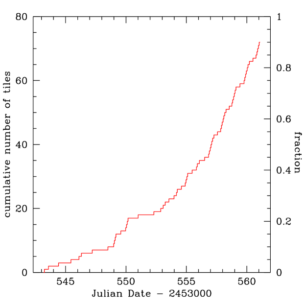
Figure 1: Cumulative plot of ACS data acquisition. In order to minimize the effects of a time-vary PSF on weak lensing applications, 50% of tiles were taken within 5 days and 90% within 21 days. The remaining 7 tiles were observed 6 months later.

Concerns about a time-varying PSF and possible effects on the weak lensing measurements drove the requirement for the observations to be taken in as short a time frame as possible. In practice this was largely successful, with $>50\%$ of tiles observed in a single five-day period (Fig. 1), and $>90\%$ within 21 days. Six tiles (29, 75, 76, 77, 79, 80) were unobservable in that cycle and were re-observed six months later, with a 180 degree rotation. Furthermore, tile 46 was also re-observed at this orientation as the original observation failed due to a lack of guide stars. These seven tiles were observed following the transition to two-gyro mode with no adverse consequences in image quality.

Details of the observations are listed in Table 1. A schematic of the field showing the ACS tiles and the multiwavelength observations is shown in Fig. 2. Additionally, four parallel observations with WFPC2 (F450W) and NICMOS3 (F110W and F160W) were obtained simultaneously for each ACS pointing. Due to the separation of different instruments on the HST focal plane, most but not all parallel images overlap with the ACS mosaic (52/10/18 WFPC images and 42/9/29 NICMOS3 images have full/partial/no overlap with the ACS mosaic; most NICMOS3 images have partial overlap with a WFPC2 image). In this paper we restrict ourselves to a discussion of the primary ACS data, analysis of the parallels will follow in a future publication.

Tile	Date	$\alpha$	$\delta$	Exposure	Nhot	Ncold	Ngood
	[dd/mm/yyyy]	[J2000]	[J2000]	[s]
1	09 07 2005	09:55:22.8	-10:14:01	1960	851	173	796
2	07 07 2005	09:55:44.5	-10:13:54	1960	1082	209	982
3	08 07 2005	09:55:33.4	-10:12:03	1960	1157	233	1008
4	07 07 2005	09:55:22.4	-10:10:06	1960	1051	199	927
5	04 07 2005	09:56:09.5	-10:14:26	1950	1069	195	973
6	03 07 2005	09:55:58.7	-10:12:33	1950	1151	219	1027
7	04 07 2005	09:55:47.9	-10:10:39	1950	1038	237	905
8	04 07 2005	09:55:37.0	-10:08:45	1950	1095	262	938
9	04 07 2005	09:55:26.2	-10:06:52	1950	1020	188	876
10	05 07 2005	09:55:15.4	-10:04:58	1950	1014	184	938
11	07 07 2005	09:56:38.6	-10:15:34	1960	989	219	876
12	04 07 2005	09:56:27.8	-10:13:40	1950	1020	226	885
13	28 06 2005	09:56:16.9	-10:11:46	2120	1193	256	1037
14	28 06 2005	09:56:06.1	-10:09:53	2120	1391	254	1111
15	28 06 2005	09:55:55.3	-10:07:59	2120	1182	253	1052
16	29 06 2005	09:55:44.5	-10:06:06	2120	1109	208	940
17	29 06 2005	09:55:33.7	-10:04:12	1960	1116	250	888
18	04 07 2005	09:55:22.9	-10:02:18	1950	995	178	868
19	09 07 2005	09:56:57.3	-10:14:25	1960	963	180	786
20	07 07 2005	09:56:46.0	-10:12:54	1960	979	222	829
21	30 06 2005	09:56:35.2	-10:11:00	1960	1166	288	1005
22	28 06 2005	09:56:24.4	-10:09:07	2120	1193	263	1012
23	25 06 2005	09:56:13.6	-10:07:13	2120	1143	241	1000
24	25 06 2005	09:56:02.8	-10:05:19	2120	1244	254	1128
25	22 06 2005	09:55:52.0	-10:03:26	2120	1274	248	1051
26	29 06 2005	09:55:41.1	-10:01:32	1960	1214	275	1063
27	05 07 2005	09:55:30.3	-09:59:39	1950	1258	279	1068
28	08 07 2005	09:55:19.5	-09:57:45	1960	1161	220	1052
29	04 01 2006	09:57:10.7	-10:14:08	2120	1274	272	1123
30	09 07 2005	09:57:04.5	-10:11:48	1960	943	209	781
31	08 07 2005	09:56:53.5	-10:10:14	1960	900	200	713
32	03 07 2005	09:56:42.7	-10:08:20	1950	1023	214	884
33	28 06 2005	09:56:31.9	-10:06:27	2120	1150	223	955
34	22 06 2005	09:56:21.0	-10:04:33	2120	1318	243	1111
35	22 06 2005	09:56:10.2	-10:02:40	2120	1220	244	1028
36	24 06 2005	09:55:59.4	-10:00:46	2120	1320	287	1101
37	29 06 2005	09:55:48.6	-09:58:53	1960	1150	239	974
38	05 07 2005	09:55:37.8	-09:56:59	1950	1123	205	951
39	08 07 2005	09:55:27.0	-09:55:05	1960	1094	210	965
40	09 07 2005	09:57:12.5	-10:09:14	1960	1062	198	916
41	07 07 2005	09:57:00.9	-10:07:34	1960	962	176	828
42	03 07 2005	09:56:50.1	-10:05:41	1950	1090	205	928
43	27 06 2005	09:56:39.3	-10:03:47	2120	1198	202	1052
44	27 06 2005	09:56:28.5	-10:01:54	2120	1266	230	1046
45	23 06 2005	09:56:17.7	-10:00:00	2120	1280	285	1064
46	01 01 2006	09:56:05.4	-09:57:47	2120	1438	355	1235
47	01 07 2005	09:55:56.0	-09:56:13	1960	1198	273	972
48	06 07 2005	09:55:45.2	-09:54:19	1950	989	176	852
49	06 07 2005	09:55:34.4	-09:52:26	1960	1054	223	901
50	09 07 2005	09:55:24.4	-09:50:31	1960	984	212	832
51	07 07 2005	09:57:08.4	-10:04:55	1960	1050	189	923
52	03 07 2005	09:56:57.6	-10:03:01	1960	1142	209	941
53	03 07 2005	09:56:46.8	-10:01:07	1950	1135	211	920
54	02 07 2005	09:56:36.0	-09:59:14	1950	1131	228	921
55	02 07 2005	09:56:25.1	-09:57:20	1960	1205	311	974
56	02 07 2005	09:56:14.3	-09:55:27	1960	1097	242	891
57	01 07 2005	09:56:03.5	-09:53:33	1960	1090	210	911
58	06 07 2005	09:55:52.7	-09:51:40	1950	1130	201	975
59	08 07 2005	09:55:32.7	-09:48:15	1960	1075	204	900
60	07 07 2005	09:57:15.8	-10:02:15	1950	1028	183	912

Table 1: Details of STAGES HST/ACS observations. Only the second (successful) acquisition of tile 46 is listed. ‘Hot’,‘cold’, and ‘good’ SExtractor configurations are described in §2.3. Tiles 29, 46, 75, 76, 77, 79, and 80 are oriented at 180° with respect to the rest of the mosaic. The exposure time varied according to the maximum window of visibility available in each orbit.

Table 2: continued

Tile	Date	$\alpha$	$\delta$	Exposure	Nhot	Ncold	Ngood
	[dd/mm/yyyy]	[J2000]	[J2000]	[s]
61	07 07 2005	09:57:05.0	-10:00:21	1950	971	183	826
62	07 07 2005	09:56:54.2	-09:58:28	1950	1052	184	901
63	06 07 2005	09:56:43.4	-09:56:34	1950	1141	217	930
64	06 07 2005	09:56:32.6	-09:54:41	1950	1069	222	890
65	06 07 2005	09:56:21.8	-09:52:47	1950	1071	227	908
66	06 07 2005	09:56:11.0	-09:50:53	1950	1014	222	859
67	06 07 2005	09:56:00.1	-09:48:60	1950	1046	226	922
68	08 07 2005	09:55:49.3	-09:47:06	1960	967	179	851
69	10 07 2005	09:57:12.5	-09:57:42	1960	876	145	784
70	09 07 2005	09:57:01.7	-09:55:48	1960	934	183	798
71	09 07 2005	09:56:50.9	-09:53:54	1960	1032	182	888
72	10 07 2005	09:56:40.0	-09:52:01	1960	1118	212	950
73	09 07 2005	09:56:29.2	-09:50:07	1960	910	168	773
74	08 07 2005	09:56:18.4	-09:48:14	1960	907	192	822
75	04 01 2006	09:57:11.0	-09:53:30	2120	1708	260	1140
76	05 01 2006	09:57:00.3	-09:51:39	2120	1444	275	1134
77	05 01 2006	09:56:49.5	-09:49:48	2120	1324	287	1094
78	05 07 2005	09:56:40.6	-09:48:11	1960	1031	184	842
79	05 01 2006	09:57:12.9	-09:50:05	2120	1357	302	1019
80	05 01 2006	09:57:02.8	-09:48:36	2120	1255	246	973

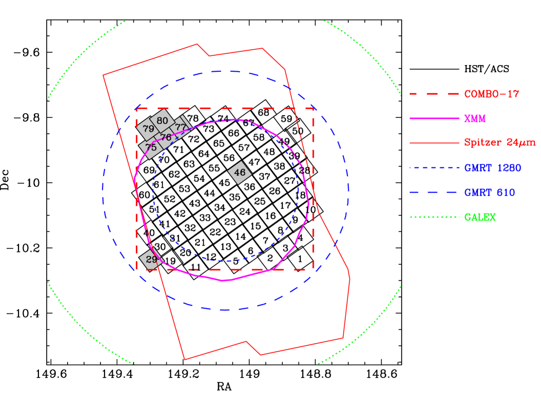
Figure 2: Layout of multiwavelength observations of the A901/2 field. The numbered tiles represent the 80-orbit STAGES mosaic with HST/ACS, which overlaps the 31.5$\times$30 arcmin COMBO-17 field-of-view (long-dashed square). The seven shaded tiles were observed $\sim$6 months after the bulk of the observations and with a 180°rotation. The centres of A901a/A901b/A902/SWG are found in tiles 55/36/21/8 respectively. Interior to the STAGES region are the XMM-Newton coverage (heavy solid polygon) and the GMRT 1280 MHz observations (short-dashed circle, indicating half-power beam width). The STAGES area is also overlapped by the field-of-view of the Spitzer 24$\micron$ imaging (solid polygon), the GMRT 610 MHz observations (long-dashed circle), and the GALEX imaging (dotted circle).

2.2 ACS data reduction

We retrieve the reduced STAGES images processed by the CALNICA pipeline of STScI, which corrects for bias subtraction and flat-fielding. However, as the ACS camera is located 6 arcmin off the centre of the HST optical axis, the images from the telescope have a field-of-view with a parallelogram keystone distortion. To produce a final science image from the reduced pipeline data, we therefore also have to remove the geometric distortion before combining the individual dithered sub-exposures. The removal of the image distortion is now fairly routine through the use of the MULTIDRIZZLE software (Koekemoer et al., 2007). However, our particular science goals motivated us to make several changes when optimizing the default settings and combining the raw images. These changes are discussed below.

2.2.1 Image Distortion Correction

In STAGES, the science driver that demands the highest quality data reduction in terms of producing the most consistent and stable PSF from image to image, and across the field of view, is weak lensing (Heymans et al., 2008). With this goal in mind, we benefit from the experience of Rhodes et al. (2007), who conducted detailed studies of how the pixel values are re-binned when the images are corrected for image distortion. Briefly speaking, to transform an image that is sampled on a geometrically distorted grid onto one that is a uniform Cartesian grid fundamentally involves rebinning, i.e. interpolating, the original pixel values into the new grid. Doing so is not a straightforward process since the original ACS pixel scale samples the telescope diffraction limit below Nyquist frequency, i.e. the telescope PSF is undersampled. When a PSF is undersampled, aliasing of the pixel fluxes occurs, the result of which is that the recorded structure of the PSF appears to change with position, depending on the exact sub-pixel centroid of the PSF. This variability effectively produces a change in the ellipticity of the PSF as a function of sub-pixel position, even if the PSF should be identical everywhere. Because stellar PSFs are randomly centred about a pixel the intrinsic ellipticity one then measures has a non-zero scatter. So, as weak lensing relies heavily on measuring the ellipticities of galaxies, which are convolved by the PSF, the scatter in the PSF ellipticity contributes significant noise to weak lensing measurements.

An additional issue with non-Nyquist sampled images is that the process of interpolating pixel values necessarily degrades the original image resolution. While the intrinsic resolution can in principle be recovered by dithering the images while making observations, strictly speaking this inversion is only possible when the image is on a perfect Cartesian grid at the start, i.e. with no image distortion. Otherwise, there would be a residual “beating frequency” in the sampling of the reconstituted image, such that some pixels would be better sampled than others. Because of this, recovering the intrinsic resolution of the telescope when the field is distorted is not a well posed problem, and cannot easily be solved by a small number of image dithers. Some resolution loss will necessarily occur in some parts of the image. This is especially true if the final images are combined after having been geometrically corrected, as is currently the process in MULTIDRIZZLE. One last, unavoidable, side effect of interpolating a non-Nyquist sampled image is that the pixel values become necessarily correlated. However, the degree of resolution loss and noise correlation can be balanced by a suitable choice of interpolation kernels: whereas square top-hat kernels effectively amounts to linear interpolation and correlates only the immediate neighbour pixels but cause high interpolation (pixellation) noise, bell-shaped kernels (e.g. Gaussian and Sinc) correlate more pixels but better preserve the image resolution.

In light of these issues, it is clear that the goal of an optimal HST data reduction should be a dataset where the PSF structure is stable across the field of view and reproducible from image tile to tile. The contribution to the PSF variation by the stochastic aliasing of the PSF that necessarily occurs during ‘drizzling’ can be reduced by appropriate choices of drizzling kernel and output pixel scale. Rhodes et al. (2007) characterize PSF stability in terms of the scatter in the apparent ellipticity of the PSF in the ACS field of view. After experimenting, they determine that the optimal set of parameters in MULTIDRIZZLE to use is a Gaussian drizzling kernel, pixfrac=0.8, and an output pixel scale of $0\aas@@fstack{\prime\prime}03$. We thus follow their approach by adopting those parameters for our own reduction, while keeping all the other default parameters unchanged. However, they note, as we do, that a Gaussian kernel causes more correlated pixels than tophat kernels. Nonetheless because the choice of interpolation kernel amounts effectively to a smoothing kernel, correlated noise should in principle not have an impact on photometry statistics since the flux is conserved. Moreover, the same interpolation (smoothing) kernel propagates into the PSF, thus the choice of kernel should also not impact galaxy fitting analyses.

2.2.2 Sky pedestal and further image flattening correction

The images obtained from the HST archive have been bias subtracted and flatfielded. However, large-scale non-flatness on the order of 2-4% remains in the images, and there are slight but noticeable pedestal offsets that remain between the four quadrants. These large scale patterns and pedestals are both stationary and consistent in images that are observed closely in time. And even though MULTIDRIZZLE tries to equalize the pedestals before combining the final images, the correction is not always perfect due to object contamination when computing the sky pedestal. These effects are small, and the sky pedestal issue only affect large objects situated right on image boundaries, so that the effects on the entire survey itself may only be cosmetic. Nevertheless, we try to correct for the effects by producing a median image of data observed closely in time, after first rejecting the brightest 30% and faintest 20% of the images (to avoid over-subtraction). Then, for each of the four CCD quadrants, we fit a low order 2-D cubic-spline surface (IRAF/imsurfit) individually to model the large scale non-uniformity in the median sky image, and to remove noise. The noiseless model of the sky is then subtracted from all the data observed closely in time. After correction, the mean background in the four quadrants is essentially equal, and the residual non-flatness is $\ll 1\%$.

2.3 Object Detection

Object detection and cataloguing were carried out automatically on the STAGES F606W imaging data using the SExtractor V2.5.0 software (Bertin & Arnouts, 1996). An optimized, dual (‘cold’ and ‘hot’) configuration was used, following the strategy developed for HST/ACS data of similar depth for GEMS (Caldwell et al., 2008). The main challenge to extracting sources from the STAGES ACS data is the tradeoff between deblending high-surface brightness cluster members that are close on the sky in projection, and avoiding spurious splitting (‘shredding’) of highly structured spiral galaxies into multiple sources. In addition, we desire high detection completeness for faint, and often low-surface brightness, background galaxies. To optimize the detection completeness and deblending reliability for counterparts to $R_{\rm ap}\leq 24$ mag galaxies from the COMBO-17 catalogue, we fine-tuned the combination of cold and hot configuration parameters using three representative STAGES tiles (21, 39, and 55). For STAGES, we converged on the parameters given in Table 3, which successfully detected 99.5% (650/653) of the $R_{\rm ap}\leq 24$ mag COMBO-17 galaxies on these tiles, with reliable deblending for 98.0%.

SExtractor produces a list of source positions and basic photometric parameters for each astrometrically/photometrically calibrated image, and produces a segmentation map that parses the image into source and background pixels, which is necessary for subsequent galaxy fitting with GALFIT (Peng et al., 2002) described in §2.4. For both configurations, a weight map ($\propto{\rm variance}^{-1}$) and a three-pixel (FWHM) top-hat filtering kernel were used. The former suppresses spurious detections on low-weight pixels, and the latter discriminates against noise peaks, which statistically have smaller extent than real sources as convolved by the instrumental PSF. Our final catalogue contains 75 805 unique F606W sources uniformly and automatically identified from 17 978 objects detected in the cold run, and 89 464 ‘good’ sources found in the hot run (before rejection of the unwanted hot detections that fell within the isophotal area of any cold detection). A total of 5 921 objects were manually removed from the catalogue after the detection stage. These detections are mainly over-deblended galaxies or image defects like cosmic rays. Another set of 658 detections were included in fitting the sample galaxies to ensure the accurate fitting of real objects, but excluded from the final catalogue. These were also mainly cosmic ray hits or stellar diffraction spikes. Although the main analysis was performed on a tile-by-tile basis, rather than mosaic-wise, the main catalogue only contains unique sources. Objects detected on two tiles enter the catalogue only once. The most interior-located was selected for entry into the catalogue. The breakdown of cold, hot, and good sources per ACS frame is given in Table 1.

In Fig. 3 we show a histogram of various object samples in the region of the HST-mosaic that overlaps with COMBO-17. The HST data start to become incomplete at $V_{606}\sim 26$ (solid line). Stars (hashed histogram) only make up a significant fraction of all detections at the brightest magnitudes. A histogram of counterparts from a cross-correlation with COMBO-17 is shown in light grey. When the match is restricted to extended objects with $R_{\rm ap}<24$ (ie. the primary ’galaxy’ sample for which we have reliable photometric redshifts), the HST sources largely have $V_{606}<24$.

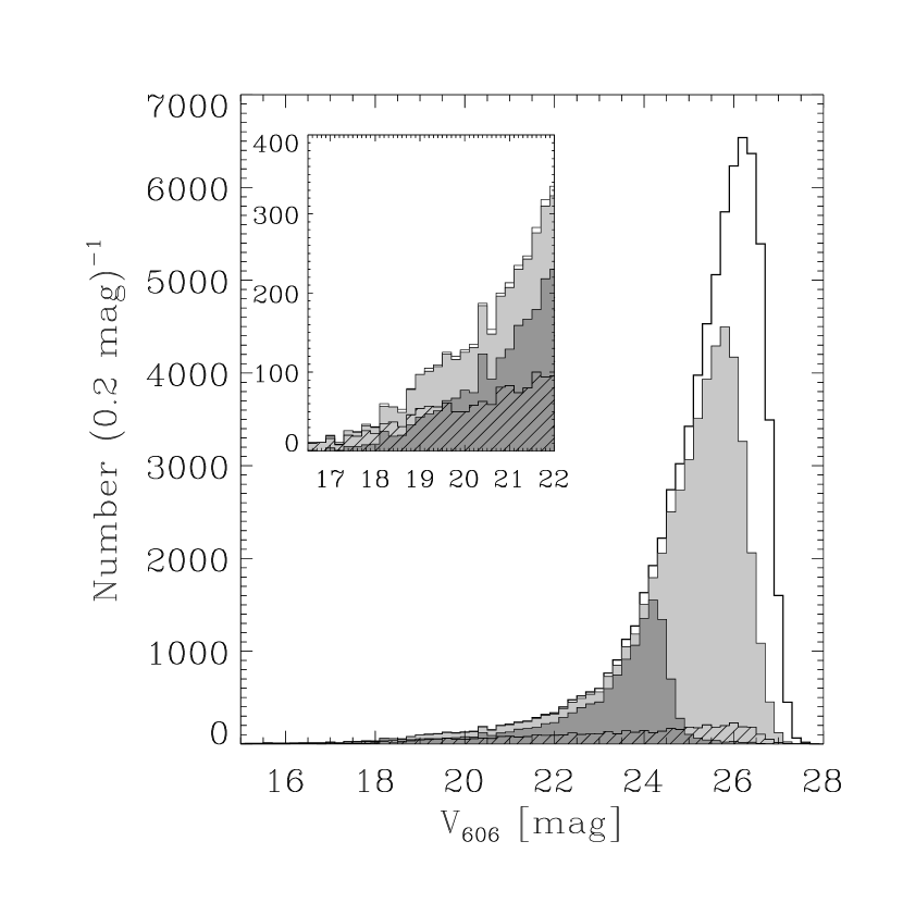
Figure 3: Source detections in the HST mosaic (overlap region with STAGES and COMBO-17 coverage). The solid line represents all SExtractor detected sources (74 534 objects). The grey histograms shows all objects with a corresponding match in the COMBO-17 catalogue (light grey; 50 701 sources) and extended sources with $R_{\textrm{ap}}<24$ (dark grey; 12 748 sources). In addition, the hashed region indicates stars as defined by our star-galaxy separation criterion (Equation 1; 4 969 stars in total). In the inset we highlight the bright magnitude end where the total number of stars dominates the source population.

Star-galaxy separation is performed in the apparent magnitude – size plane spanned by the SExtractor parameters MAG_BEST ($V_{606}$) and FLUX_RADIUS ($r_{f}$). Objects with

$$\log(r_{f})<{\rm max}\left(0.35;1.60-0.05V_{606};5.10-0.22V_{606}\right)$$ (1)

are classified as point sources; sources above that line are identified as extended sources (galaxies). This plane is shown in Fig. 4. The separation line clearly delineates compact and extended sources, in particular when inspecting the COMBO-17 sources only (crosses). Note that those AGN for which the point source dominates are also found on the point-source locus and therefore are removed from the galaxy sample by this selection.

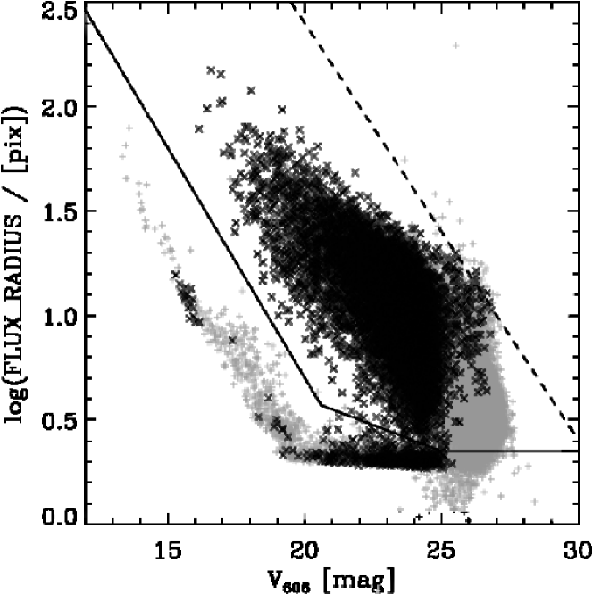
Figure 4: Star-galaxy separation. We define a line in the magnitude-size plane to separate stars and galaxies (solid line). Objects above this line are extended galaxies; objects below are other compact objects (including most AGN). Grey pluses indicate all detections; black crosses only those with a COMBO-17 cross-match and $R_{\textrm{ap}}<24$ and a redshift $z>0$. Note, a significant number of mostly late-type stars are misidentified as galaxies by COMBO-17 photometry alone. The dashed line shows a line of constant surface brightness, which is almost parallel to our selection line at the bright end.

In the Fig. 5 we display the galaxy fraction as a function of $V_{606}$ magnitude (grey histogram). Out to $V_{606}\sim 22$ almost every galaxy detection on the HST images has a COMBO-17 counterpart; at the COMBO-17 sample limit $V_{606}\sim 24$ the matching completeness for STAGES objects is still $\sim$90%. The cross-matching between COMBO-17 and the HST data is described in more detail in § 3.2, where completeness is defined in reverse, i.e. maximizing HST counterparts for COMBO-17 objects.

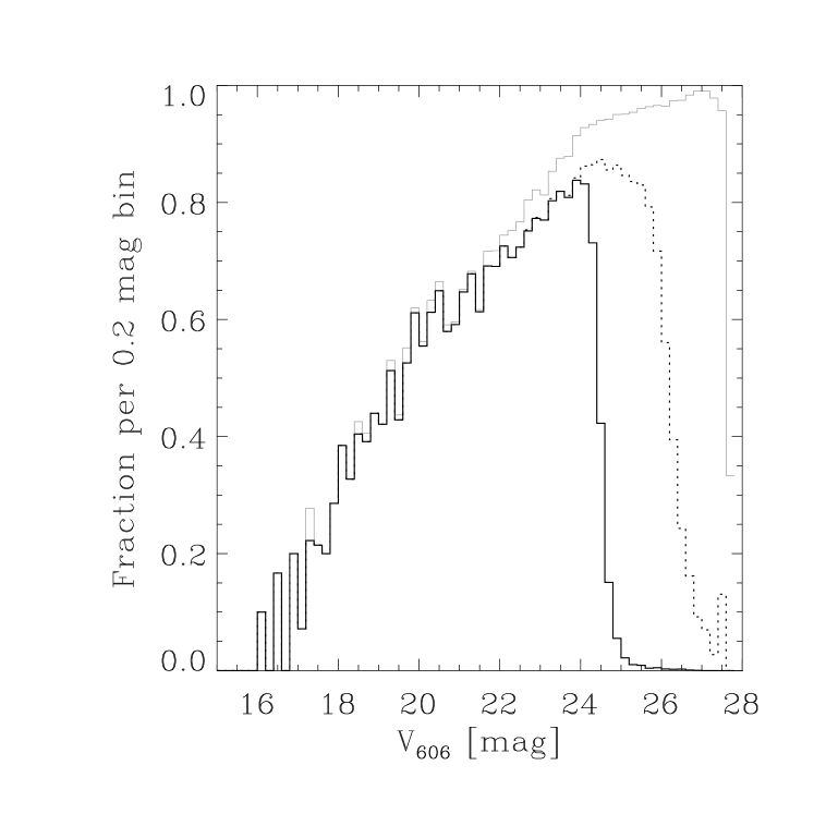
Figure 5: Fraction of extended STAGES objects and COMBO-17 counterparts. The grey line shows the extended source fraction in STAGES. At bright magnitudes most sources are compact, while at the faint end almost all are extended. The black dotted line shows extended sources in STAGES with a COMBO-17 counterpart. At $V_{606}\sim 26$ the COMBO-17 completeness limit is reached. Almost no fainter sources are found in COMBO-17. The black solid line shows extended sources in STAGES with a COMBO-17 counterpart having $R_{\textrm{ap}}<24$. Out to $V_{606}\sim 22$ almost every extended STAGES object has a COMBO-17 counterpart: the cross-correlation completeness defined with respect to the STAGES catalogue is almost 100% (i.e. the ratio of black and grey lines); at $V_{606}\sim 24$ it is $\sim$90%. See §3.2 for further discussion.

Table 3: Dual SExtractor parameter values for STAGES F606W object detection in ‘cold’ and ‘hot’ configurations.

Parameter	Cold	Hot	Description
DETECT_THRESH	2.8	1.5	detection threshold above background
DETECT_MINAREA	140	45	minimum connected pixels above threshold
DEBLEND_MINCONT	0.02	0.25	minimum flux/peak contrast ratio
DEBLEND_NTHRESH	64	32	number of deblending threshold steps

2.4 Sérsic profile fitting

To obtain Sérsic model fits for each STAGES galaxy, the imaging data were processed with the data pipeline GALAPAGOS (Galaxy Analysis over Large Areas: Parameter Assessment by GALFITting Objects from SExtractor; Barden et al., in prep.). GALAPAGOS performs all galaxy fitting analysis steps from object detection to catalogue creation automatically. This includes (i) source detection and extraction with SExtractor; (ii) preparing all detected objects for Sérsic fitting with GALFIT (Peng et al., 2002): i.e., constructing bad pixel masks, measuring local background levels, and setting up starting scripts with initial parameter estimates; (iii) running the Sérsic model fits; and (iv) compiling all information into a final catalogue.

Based on a single startup script, GALAPAGOS first runs SExtractor in the dual high dynamic range mode described in §2.3. As no SExtractor setup is ever 100% optimal, we manually inspected all 80 tiles for unwanted detections or over-deblended objects. GALAPAGOS allows for the removal of such extraction failures automatically given an input coordinate list. Additionally, we also composed a list of detections that are bright enough to influence the fitting of neighbouring astronomical sources (e.g. diffraction spikes from bright stars). Unlike the aforementioned bad detections these are not removed instantly, but kept in the source catalogue throughout the fitting process and removed only from the final object catalogue. Again, GALAPAGOS performs this operation automatically given a second list of coordinates. Further details on the process of manual fine-tuning of detection catalogues can be found in Barden et al. (in prep.).

After the second run GALAPAGOS uses the cleaned output source list (described in §2.3) to cut postage stamps for every object. Postage stamps are required for efficient Sérsic profile fitting with GALFIT. The sizes of the postage stamps are based on a multiple $m$ of the product of the SExtractor parameters KRON_RADIUS and A_IMAGE. We define a “Kron-ellipse” with semi-major axis $r_{\textrm{K}}$ as

$$r_{\textrm{K}}=m\times\textrm{KRON\_RADIUS}\times\textrm{A\_IMAGE}.$$ (2)

The sky level is calculated for each source individually by evaluating a flux growth curve. GALAPAGOS uses the full science frame for this purpose in contrast to simply working on the postage stamp. Although in principle the background estimate provided by SExtractor could have been used, tests show that using the more elaborate GALAPAGOS scheme results in more robust parameter fits (Häussler et al., 2007). For a detailed description of the algorithm we refer to Barden et al. (in prep.). One might argue that GALFIT allows fitting the sky simultaneously with the science object. However, this requires the size of the postage stamp to be matched exactly to the size of the science object. If the postage stamp is too small, the proper sky value cannot be found; if it is too big, computation takes unneccesarily long. Too many secondary sources would have to be included in the fit and the inferred sky value might be influenced by distant sources. Additionally, galaxies may not be perfectly represented by a Sérsic fit, and the sky may take on unrealistic values as a result. Although this method may be the easiest option for manual fitting, in the general case of fitting large numbers of sources automatically the most robust option is to calculate the sky value beforehand and keep its value fixed when running GALFIT (as demonstrated in Häussler et al., 2007).

Another crucial component for setting up GALFIT is determining which companion objects should be included in the fit. In particular, in crowded regions with many closely neighbouring sources the fit quality of the primary galaxy improves dramatically when including simultaneously fitting Sérsic models to these neighbours rather than simply masking them out. GALAPAGOS makes an educated guess as to which neighbours should be fitted or masked (see Barden et al., in prep. for further details). The decision is made by calculating whether the Kron-ellipses of primary and neighbouring source overlap. This calculation is performed not only for sources on the postage stamp, but on all objects on the science frames surrounding the current one, in order to take objects at frame edges into account properly. Detections not identified as overlapping secondary sources are treated as well. Such non-overlapping companions are masked based on their Kron-ellipse and thus excluded from fitting.

An additional requirement for fitting with GALFIT is an input PSF. We constructed a general high S/N PSF for STAGES by combining all stars (i.e. classified by COMBO-17 photometry and having ACS SExtractor stellarity index $>0.85$) in the brightness interval $19.5<V_{606}\leq 23.5$ and lying away from the chip edges. This selects non-saturated stars that can still contribute signal in their centres. All stars were visually inspected against binarity, companions, or defects, which resulted in either a manually created mask, or the star being excluded if masking would not have been sufficient to isolate the star. With this selection 1 024 stars remained and were combined after subpixel cocentering and local background removal.

In order to sample the field-variations of the PSF well and not be dominated by the few brightest stars, we weighted all stars identically in the centre (where all stars carry information), but applied a suppression of the noise in the outer parts by a Gaussian downweighting. The contribution from fainter stars in this process was suppressed at smaller radii relative to brighter ones. In this way we created a high S/N true mean PSF image of 255$\times$255 pixel centred exactly on the PSF and used this for all galaxy-related (but not AGN related) analyses.

In its current version, GALAPAGOS sets up GALFIT to fit a Sérsic model (Sersic, 1968) for each object. A Sérsic profile is a generalised de Vaucouleurs model with variable exponent $n$, the Sérsic index:

$$\Sigma\left(r\right)=\Sigma_{e}\times\exp\left(-\kappa\left[\left(r/r_{e}\right)^{1/n}-1\right]\right),$$ (3)

with the effective radius $r_{e}$, the effective surface density $\Sigma_{e}$, the surface density as a function of radius $\Sigma\left(r\right)$ and a normalisation constant $\kappa=\kappa\left(n\right)$. An exponential profile has $n=1$ while a de Vaucouleurs profile has $n=4$. The parameters that go into the model are the position $[x,y]$, total magnitude $m$, the effective radius $r_{e}$, the Sérsic index $n$, the axis ratio $q$ ($q=b/a$; the ratio of semi-minor over semi-major half-axis ratio) and the position angle $\theta$. Starting guesses for all parameters aside from $n$ and $r_{e}$ are taken directly from the SExtractor output. GALAPAGOS converts the FLUX_RADIUS from SExtractor to estimate the effective radius as $r_{e}=10^{-0.79}\textrm{FLUX\_RADIUS}^{1.87}$. This formula was found empirically to work best for simulated Sérsic profiles in the GEMS project (Häussler et al., 2007). The Sérsic index is started at a value $n=2.5$.

For computational efficiency we apply constraints to the parameter range during the fitting process. Of course, this procedure is not advisable when fitting objects manually, yet it is mandatory for an automated process like GALAPAGOS. Our constraints are listed in Table 4. Non-zero lower boundaries for $r_{e}$ and $n$ were imposed for computational reasons. The maximum for $r_{e}$ allows fitting the largest galaxy in the field (750 pix correspond to $\sim 60$ kpc at the cluster distance). The upper limit for the Sérsic index is far from the de Vaucouleurs case and includes even the steepest profiles. The magnitude constraint flags catastrophic disagreements between the two photometry codes, where one of the two does not return a sensible result. Such problem objects may include LSB galaxies, where SExtractor fails to see large fractions of the total flux; or intrinsically faint objects with a peculiar neighbour or background structure, where GALFIT tries to remove the excess flux. Objects whose values stall at the constraint limits are most likely not well represented by a single Sérsic profile (e.g. stars or extreme two-component galaxies with a LSB disk).

Table 4: GALFIT fitting constraints.

Parameter	Lower limit	Upper limit
$r_{e}$	0.3	750
$n$	0.2	8
$|m_{\rm SEx}-m_{\rm GALFIT}|$	-	5

Finally, GALAPAGOS combines the SExtractor and GALFIT results into one FITS-table. At this stage flagged objects (like stellar diffraction spikes, etc.) are removed from the table. A very detailed description of GALAPAGOS including setup and computational efficiency will be presented together with the publication of the code in Barden et al. (in prep.). We note that the GALFIT reported errors are purely statistical (ie. based on the assumption that Poisson noise dominates the uncertainties of the fit parameters), and as such certainly under-represent the true uncertainties. A more meaningful measure of uncertainties comes from fitting simulated galaxies, as shown in Häussler et al. (2007) and explored here in detail in §2.5.

With our setup we were able to achieve an overall total of $\sim 92$% high quality fits for our science targets, i.e. galaxies with a cross-match in the COMBO-17 catalogue and $R_{\textrm{ap}}<24$. We define ‘bad’ fits as those where GALFIT stalled at one of the constraints in Table 4. In Fig. 6 we show the fraction of those bad fits as a function of SExtractor magnitude. At the bright end ($V_{606}<22$), the fraction of failures is less than 6% and rises steadily from there. Only when reaching the (surface brightness) completeness limit (roughly at $V_{606}\sim 24-25$) does the fraction of failed fits reach (and exceed) 20%.

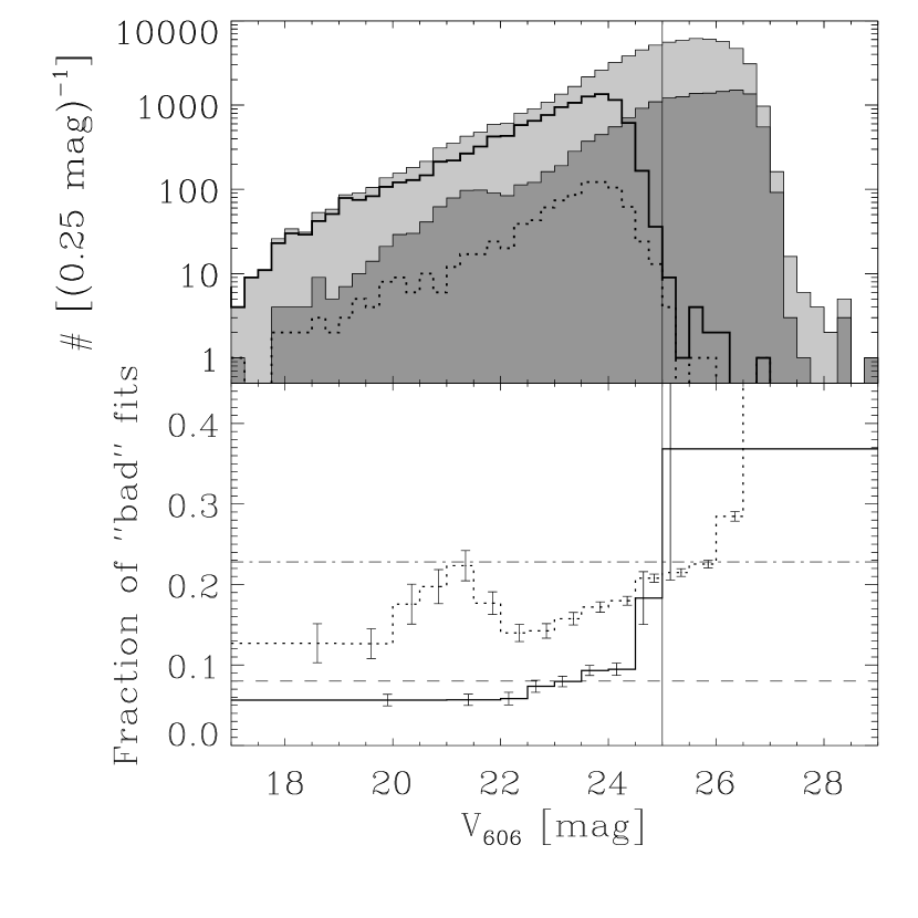
Figure 6: GALFIT quality. Top panel: The two grey histograms show the total number of fitted galaxies (light grey) and galaxies with ‘bad’ fits where the fitting procedure failed (dark grey). The heavy solid and dotted histograms show the same but for the science sample with $R_{\textrm{ap}}<24$ (i.e. objects with a COMBO-17 counterpart only) within the overlap region of STAGES and COMBO-17. Bottom panel: Fraction of ‘bad’ fits (plus 1$\sigma$ error bars) for all fitted galaxies (dotted histogram) and those with a COMBO-17 match and $R_{\textrm{ap}}<24$ (solid histogram). Overall, $\sim 23$% of all fits ran into a constraint (dashed dotted line). For the science objects (STAGES/COMBO-17 cross-matched galaxies with $R_{\textrm{ap}}<24$) the fraction is considerably lower ($\sim 8$%; dashed line). The vertical line roughly indicates the surface brightness completeness limit. The ‘bump’ at $V_{606}\sim 21$ possibly results from merging two SExtractor setups (the ‘hot’ and ‘cold’ configurations described in §2.3).

2.5 Completeness and Fit Quality

To both derive completeness maps and examine fitting quality using GALAPAGOS, we followed a similar approach as in GEMS and as described in Häussler et al. (2007), but with a different, more realistic set of simulated data. Whereas in Häussler et al. (2007) a small set of only 1 600 simulated galaxies was used to find the ideal setup of the fitting pipeline, we have now decided on a fitting setup using GALAPAGOS from the start and have carried out much more intensive tests. We created entire sets of STAGES-like imaging data by simulating galaxies in all 80 HST/ACS tiles. Galaxies were simulated as single-component Sérsic profiles; multi-component galaxies or complicated structures such as spiral arms or bars were not included.

The sample of galaxies to be simulated was derived by using the fits of real data as described in §2.4. From this superset, we selected a ‘galaxy sample’ to be simulated by excluding both stars and those galaxies for which the fit failed. Magnitudes and galaxy sizes for the simulated galaxies were chosen according to the probability distribution of this sample. The other simulation parameters, (e.g. Sérsic index $n$ and axis ratio $q$) were then derived by choosing fitting values of real galaxies at approximately the same magnitude and size. In this way, the simulated data have parameters as close as possible to the real galaxy sample.

To cover a larger number of parameter combinations, we slightly smoothed these values (mag by $\pm$1 mag, $\log(r_{e})$ by $\pm$0.25 pix, $n$ by $\pm$0.5 and $q$ by $\pm$0.2). Care was taken to make sure that $q$ and $n$ covered sensible values ($0.05<q<1$, $0.2<n<8$). We also simulated galaxies two magnitudes fainter than those found in the real data to be able to derive completeness maps from the same pipeline. Twenty sets of STAGES-like data (80 tiles each) were simulated using this setup. In a further 50 sets, we introduced a uniform distribution of the Sérsic index over the full range $0.2<n<8$ over all magnitudes and sizes for 5% of galaxies. This imposed pedestal was required in order to fill in gaps in the parameter space with bad number statistics or no galaxies at all, and was especially important for galaxies with high $n$-value seen face-on. Both position and position angle, $\theta$, were randomly chosen for each galaxy: thus no clustering was simulated, in contrast to the real data. Simulating around 107 000 objects per dataset, we were able to derive an object density comparable to the real data with a mean of 60 612 galaxies found per dataset. This compares to 75 805 galaxies in the original GALAPAGOS output from the real data, with $\sim$35 000 objects in the ‘galaxy’ catalogue from which we draw the input parameters for the simulations.

After choosing the parameters this way, we used the same simulation script that was described in detail in Häussler et al. (2007) to simulate the galaxies. The images were placed in an empty image which was made up by empty patches of sky from the STAGES data to resemble the noise properties of the real data. Convolution was performed using a STAGES PSF. In a change to the Häussler et al. (2007) setup, we also simulated galaxies on neighbouring tiles (or closely outside the data area) to realistically model effects from neighbouring galaxies, as well as to examine effects of combining the individual SExtractor catalogues within GALAPAGOS.

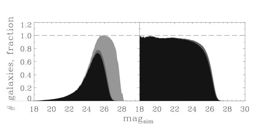
Figure 7: Completeness as a function of magnitude. Left: the number of simulated galaxies (light grey), recovered by SExtractor (dark grey), and subsequently fit successfully by GALAPAGOS (black) as a function of input magnitude. Right: Completeness functions for SExtractor (grey) and GALAPAGOS (black) output. One can see that GALAPAGOS returns a useful result in most cases. Only for relatively faint galaxies does the fit run into fitting constraints for a fraction of the objects. At $V_{606}\sim 26$, the STAGES profile fitting is therefore 80% complete.

By simulating fainter galaxies than are found in the real data, we were not only able to test the fitting quality but also the survey completeness. Fig. 7 shows the completeness as derived from this data as a function of magnitude. The left plot shows the number of galaxies simulated (light grey), the number of galaxies recovered (dark grey) and the number of galaxies with successful fit (black; meaning that the fit did not run into any fitting constraints). All three histograms are normalized by the value of the bin containing the maximum number of simulated galaxies. In total, of the 7 497 614 galaxies simulated, 43.4% were not found in the data using the GALAPAGOS and SExtractor setups used to analyse the real STAGES data. Failed objects in general were too faint to be detected. A further 52.5% were successfully recovered, identified and fitted, and 4.0% were recovered but excluded from all plots as the fit ran into fitting constraints. For 305 galaxies (0.004%), the fit crashed and did not return a result at all.

We additionally find 51 043 galaxies (0.7% of simulated galaxies) that could not be identified by our search algorithm, which looked for the closest match within 1.0″. Examination of these galaxies shows that they are either (a) very low surface brightness galaxies for which the SExtractor positioning was not very secure, or (b) two neighbouring LSB galaxies that SExtractor detected as one object, also resulting in an insecure position.

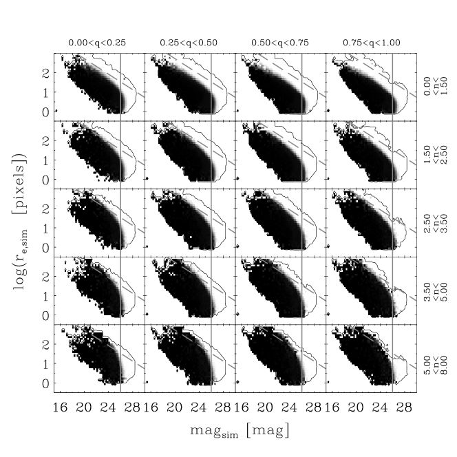
Figure 8: Completeness maps as a function of Sérsic index $n$ and axis ratio $q$ (as labelled above and to the right of the plots). To guide the eye, we overplot a vertical line at mag 26 and a surface brightness line (diagonal, dashed) at 28 mag arcsec^-2. As one can clearly see, the completeness (shown in greyscale, black is complete, white is incomplete or no data) is a strong function of all magnitude, size (and therefore surface brightness), $q$ and $n$. The outline contour shows the region in this plot where galaxies have been simulated to demonstrate where these plots are reliable.

Using the whole available simulated dataset, we can derive a much more detailed completeness for STAGES. Magnitude alone is not a good estimator for completeness, as the internal light distribution has great influence on this value. More concentrated galaxy profiles, such as elliptical, high-$n$ profiles, are more likely to be detected by SExtractor than disk-like low-$n$ profiles. In addition, the inclination angle plays an important role. As shown in Fig. 8, we can divide the galaxies in different bins of $n$ and $q$ and for each bin can estimate a 2-D completeness map showing the completeness as a function of both magnitude and galaxy size. By looking at each bin one can clearly see that the completeness is indeed a function of magnitude as well as size. The completeness catalogue from these extensive simulations will be made publicly available as part of the STAGES data release. With the large sample and complete coverage of the parameter space populated by real galaxies, one could make up customized completeness maps tailored to the particular sample in question.

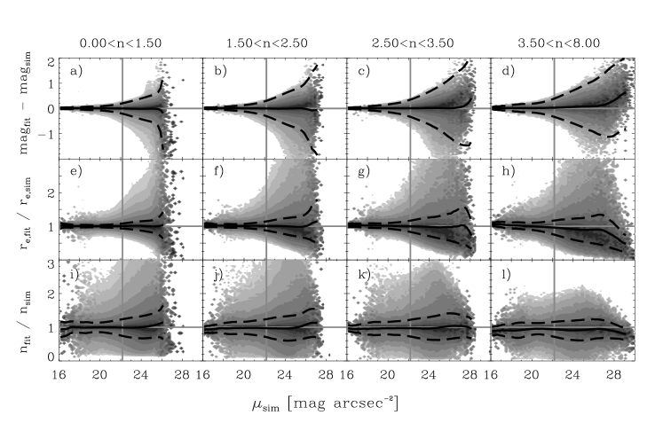
Figure 9: Fit Quality. The deviations of the most important galaxy parameters as a function of surface brightness. Top row: Magnitude deviation (fit - simulated), middle row: Size ratio (fit/simulated), bottom row: Sérsic index n (fit/simulated). Contours show the data normalized by the number of galaxies in each surface brightness bin; the black solid line shows the mean of the distribution; and the black dashed lines show the sigma of the distribution ($3\sigma$ in case of magnitudes, $1\sigma$ in size and Sérsic index). All plots are shown for different Sérsic indices as labelled above the plots. The vertical grey line represents the mean brightness of the sky background in STAGES. The magnitude and sizes are less well recovered in high-$n$ galaxies, but the relative recovery of $n$ is similar in all cases.

The same is true for the fitting quality. As can be seen from Fig. 9, the fitting behaviour is a function of both surface brightness and Sérsic index. We only show the quality as a function of Sérsic index, but again one can determine fitting quality as a function of any combination of the fitted parameters. One can see that high-$n$ galaxies are harder to fit than low-$n$ galaxies, e.g. the magnitude deviation $\Delta$ is 0.00 ($\sigma=0.07$) at around the sky level for galaxies with $0<n<1.5$, while $\Delta=0.03$ ($\sigma=0.12$) at the highest $n$-bin. The effect is even larger at fainter galaxies: $\Delta=0.00$ ($\sigma=0.18$) at 25 mag arcsec^-2and $\Delta=0.08$ ($\sigma=0.28$) for low- and high-$n$ galaxies, respectively. A similar trend can be seen for galaxy sizes: $\Delta=0.8\%$ ($\sigma=7.3\%$) and $\Delta=-3.7\%$ ($\sigma=19.0\%$) at the sky level, and $\Delta=-0.4\%$ ($\sigma=18.3\%$) and $\Delta=-10.7\%$ ($\sigma=36.1\%$) at 25 mag arcsec^-2. If one examines relative deviations of the Sérsic index, there is essentially no trend seen between different bins of $n$. In an absolute sense, then, the Sérsic index is still less well recovered in the high-$n$ bin.

In general, the systematic deviations are very small except at the faintest galaxies detectable, and both deviation $\Delta$ and $\sigma$ of the distributions are well understood within STAGES. As was pointed out in Häussler et al. (2007), the uncertainties returned by GALFIT (and therefore GALAPAGOS) underestimate the true uncertainty by a large amount. Using a statistical approach therefore returns more reliable errorbars for the individual parameters. The simulations and catalogue presented here allow a flexible means of estimating errors on profile fitting for any possible subsample of galaxies.

3 COMBO-17 data

3.1 COMBO-17 observations and catalogue

In this section we briefly describe the COMBO-17 data on the A901/2 field, including observations, catalogue entries and object samples. The corresponding data on the CDFS field were published in Wolf et al. (2004, hereafter W04), where further technical details can be found.

The filter set (Table 5) contains five broad-band filters (UBVRI) and 12 medium-band filters covering wavelengths from 350 to 930 nm. All observations were obtained with the Wide Field Imager (WFI) at the MPG/ESO 2.2m-telescope on La Silla, Chile. A field of view of $34\arcmin\times 33\arcmin$ (see Fig. 2) is covered by a CCD mosaic consisting of eight 2k $\times$ 4k CCDs with a scale of $0\aas@@fstack{\prime\prime}238$ per pixel. The observations on the A901/2 field were spread out over three observing runs between January 1999 and February 2001. They encompass a total exposure time of $\sim$185 ks of which $\sim$20 ks were taken in the $R$-band during the best seeing conditions. A dither pattern with at least ten telescope pointings spread by $\Delta\alpha$, $\Delta\delta<\pm 72\arcsec$ allowed us to cover the sky area in the gaps of the CCD mosaic.

Table 5: COMBO-17 imaging data on the A901/2 field: For all filters we list total exposure time, average PSF among individual frames, the 10$\sigma$ (Vega) magnitude limits for point sources and the observing runs (see Tab. 6) in which the exposure was collected. For flux and magnitude conversions we list AB magnitudes and photon fluxes of Vega in all filters. The $R$-band observations were taken in the best seeing conditions.

$\lambda_{\mathrm{\mathrm{cen}}}$/fwhm		$t_{\mathrm{\mathrm{exp}}}$	seeing	$m_{\mathrm{\mathrm{lim},10\sigma}}$	run code	mag of Vega	$F_{\mathrm{phot}}$ of Vega
(nm)		(sec)		(Vega mags)		(AB mags)	$(10^{8}~{}\mathrm{photons/m^{2}/nm/s})$
365/36	$U$	22100	1$\aas@@fstack{\prime\prime}$10	23.7	G	$+0.77$	0.737
458/97	$B$	20500	1$\aas@@fstack{\prime\prime}$20	25.4	A, G	$-0.13$	1.371
538/89	$V$	6000	1$\aas@@fstack{\prime\prime}$20	24.3	E	$-0.02$	1.055
648/160	$R$	20300	0$\aas@@fstack{\prime\prime}$75	25.0	E	$+0.19$	0.725
857/147	$I$	7500	1$\aas@@fstack{\prime\prime}$00	22.7	E	$+0.49$	0.412
418/27		7300	1$\aas@@fstack{\prime\prime}$20	24.0	E	$-0.19$	1.571
462/13		10000	1$\aas@@fstack{\prime\prime}$20	23.7	E	$-0.18$	1.412
486/31		5500	1$\aas@@fstack{\prime\prime}$15	24.0	E	$-0.06$	1.207
519/16		6000	1$\aas@@fstack{\prime\prime}$05	23.6	E	$-0.06$	1.125
572/25		5000	0$\aas@@fstack{\prime\prime}$85	23.5	E	$+0.04$	0.932
605/21		6000	0$\aas@@fstack{\prime\prime}$95	23.4	E	$+0.10$	0.832
645/30		4950	1$\aas@@fstack{\prime\prime}$30	22.7	E	$+0.22$	0.703
696/21		6600	1$\aas@@fstack{\prime\prime}$00	22.7	E	$+0.27$	0.621
753/18		7000	1$\aas@@fstack{\prime\prime}$05	22.2	E	$+0.36$	0.525
816/21		19200	0$\aas@@fstack{\prime\prime}$85	22.8	A	$+0.45$	0.442
857/15		16600	1$\aas@@fstack{\prime\prime}$15	21.7	E	$+0.56$	0.386
914/26		15700	0$\aas@@fstack{\prime\prime}$95	21.9	E	$+0.50$	0.380

Table 6: COMBO-17 observing runs with A901/2 imaging.

COMBO-17 run code	Dates
A	11.02.-22.02.1999
E	28.01.-11.02.2000
G	19.01.-20.01.2001

Flux calibration was done with our own tertiary standard stars based on spectrophotometric observations, a suitable method to achieve a homogeneous photometric calibration for all 17 WFI filter bands. Two G stars with $B\simeq 15$ (with COMBO-17 identification numbers 45811 and 46757) were observed at La Silla with DFOSC at the Danish 1.54 m telescope. A wide ($5\arcsec$) slit was used for the COMBO-17 standards as well as for an external calibrator star.

The object search for the COMBO-17 sample was done with SExtractor software (Bertin & Arnouts, 1996) in default setup, except for choosing a minimum of 12 significant pixels required for the detection of an object. We first search rather deep and then clean the list of extracted objects of those having a S/N ratio below 4, which corresponds to $>0\aas@@fstack{m}2422$ error in the total magnitude MAG_BEST. As a result we obtained a catalogue of 63 776 objects with positions, morphology, total $R$-band magnitude and its error. The astrometric accuracy is better than $0\aas@@fstack{\prime\prime}15$. Using our own aperture photometry we reach a 5$\sigma$ point source limit of $R\approx 25.7$.

We obtained spectral energy distributions of all objects from photometry in all 17 passbands by projecting the known object coordinates into the frames of reference of each single exposure and measuring the object fluxes at the given locations. In order to optimize the signal-to-noise ratio, we measure the spectral shape in the high surface brightness regions of the objects and ignore potential low surface brightness features at large distance from the centre. However, this implies that for large galaxies at low redshifts $z<0.2$ we measure the SED of the central region and ignore colour gradients.

Also, we suppressed the propagation of variations in the seeing into the photometry by making sure that we always probe the same physical footprint outside the atmosphere of any object in all bands irrespective of the PSF. Here, the footprint $f(x,y)$ is the convolution of the PSF $p(x,y)$ with the aperture weighting function $a(x,y)$. If all three are Gaussians, an identical physical footprint can be probed even when the PSF changes, simply by adjusting the weighting function $a(x,y)$. We chose to measure fluxes on a footprint of $1\aas@@fstack{\prime\prime}5$ FWHM outside the atmosphere ($\sim 4.2$ kpc at $z\sim 0.165$). In detail, we use the package MPIAPHOT (Meisenheimer & Röser, 1993) to measure the PSF on each individual frame, choose the weighting function needed to conserve the footprint and obtain the flux on the footprint. Fluxes from individual frames are averaged for each object and the flux error is derived from the scatter. Thus, it takes not only photon noise into account, but also suboptimal flatfielding and uncorrected CCD artifacts.

All fluxes are finally calibrated by the tertiary standards in our field. The aperture fluxes correspond to total fluxes for point sources, but underestimate them for extended sources. The difference between the total (SExtractor-based) and the aperture (MPIAPHOT-based) magnitude is listed as an aperture correction and used to calculate e.g. luminosities. For further details on the observations and the data processing, see W04.

The A901/2 field is affected by substantial foreground dust reddening at the level of $E(B-V)\approx 0.06$, in contrast to the CDFS. Hence, any SED fitting and derivation of luminosities requires dereddened SEDs. Therefore, in the catalogue we list three sets of photometry:

1. $R$-band total and aperture magnitudes as observed for the definition of samples and completeness;

2. aperture fluxes $F_{\rm phot}$ in 17 bands, dereddened using $A_{V}=0.18$ and $(A_{U},A_{B},A_{R},A_{I})=A_{V}\times(1.63,1.24,0.82,0.6)$ with similar numbers for medium-band filters (rereddening with these numbers would restore original measurements); and

3. aperture magnitudes (Vega) in all 17 bands, dereddened, on the Asinh system (Lupton et al., 1999) that can be used for logarithmic flux plots with no trouble arising from formally negative flux measurements.

Fluxes are given as photon fluxes $F_{\mathrm{phot}}$ in units of photons/m²/s/nm, which are related to other flux definitions by

$$\nu F_{\nu}=hcF_{\rm phot}=\lambda F_{\lambda}~{}.$$ (4)

Photon fluxes are practical units at the depth of current surveys. A magnitude of $V=20$ corresponds to 1 photon/m²/s/nm in all systems (AB, Vega, ST), provided $V$ is centred on 548 nm. Flux values of an object are missing in those bands where every exposure was saturated.

The final catalogue contains quality flags for all objects in an integer column (‘phot_flag’), holding the original SExtractor flags in bit 0 to 7, corresponding to values from 0 to 128, as well as some COMBO-17 quality control flags in bits 9 to 11 (values from 512 to 2048). We generally recommend that users ignore objects with flag values phot_flag $\geq 8$ for any statistical analysis of the object population. If an object of particular interest shows bad flags, it may still have accurate COMBO-17 photometry and could be used for some purposes. Often only the total magnitude was affected by bright neighbours, while the aperture SED is valid.

We then employ the usual COMBO-17 classification and redshift estimation by template fitting to libraries of stars, galaxies, QSOs and white dwarfs. There, the error rate increases very significantly at $R_{\rm ap}>24$. We refer again to W04 for details of the libraries and known deficiencies of the process, but repeat here (and correct a misprint in W04) the definition of the classifications (see Table 7).

Table 7: Definition of entries for the ‘mc_class’ column and comparison of object numbers between the COMBO-17 data sets of the A901/2 and CDFS field. The samples refer to a magnitude range of $R_{\rm ap}=[16,24]$ and only objects with phot_flag$<8$. The A901/2 field is richer in stars because of its galactic coordinates. It is also richer in galaxies due to the cluster, while the CDFS is underdense at $z=[0.2,0.4]$. We note that these definitions are based on the COMBO-17 data SED and morphology; star-galaxy separation employing morphological information from the HST imaging (Equation 1) is considered separately.

Class entry	Meaning	$N\_{\rm A901/2}$	$N\_{\rm CDFS}$
Star	stars	2096	992
	(only point sources)
WDwarf	white dwarf	14	9
	(only point sources)
Galaxy	galaxies	14555	11054
	(shape irrelevant)
Galaxy (Star?)	binary or low-z galaxy	44	46
	(star SED but extended;
	ambiguous colour space)
Galaxy (Uncl!)	SED fit undecided	316	243
	(most often galaxy)
QSO	QSOs	73	66
	(only point sources)
QSO (Gal?)	Seyfert-1 AGN or	36	31
	interloping galaxy
	(AGN SED but extended;
	ambiguous colour space)
Strange Object	unusual strange spectrum	1	3
	($\chi^{2}_{\rm red}>30$)

We also show in Table 7 a comparison of the sample sizes in different classes between the A901/2 and the CDFS field of COMBO-17. The main difference is that the A901/2 field contains more than twice the number of stars given its position at relatively low galactic latitude ($+33.6\deg$). Another difference is that it contains 30% more galaxies than the CDFS, which is both a consequence of the cluster A901/2 and the underdensity in the CDFS seen at $z\sim[0.2,0.4]$. Fig. 10 shows a colour-magnitude diagram of the star and white dwarf sample as well as redshift-magnitude diagrams for galaxies and QSOs.

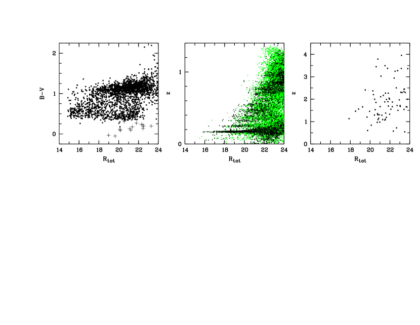
Figure 10: Left panel: Stars (dots) and white dwarfs (crosses): $B-V$ colour vs. $R_{\rm tot}$. The two reddest stars at $R\approx 23$ and $B-V>2$ are M5-6 stars. Centre panel: Red-sequence (black) and blue-cloud galaxies (green): MEV redshift vs. $R_{\rm tot}$. Right panel: QSOs: MEV redshift vs. $R_{\rm tot}$.

Redshifts are given as Maximum-Likelihood values (the peak of the PDF), or as Minimum-Error-Variance values (the expectation value of the PDF). MEV redshifts have smaller true errors, but are only given when the width of the PDF is lower than $\sigma_{z}/(1+z)<0.125$. If PDFs are bimodal with modes of sufficiently small width, then both values are given with the preferred (larger-integral) mode providing the primary redshift. Our team uses only MEV redshifts (with column name ‘mc_z’) for their analyses.

The galaxy sample with MEV redshifts is $>90$% complete at all redshifts for $R_{\rm ap}<23$. Near $z\sim 1$, the MEV redshifts are this complete even at $R_{\rm ap}=24$. Below this cut, increasing photon noise drives an expansion of the width of the PDF. The error limit for MEV redshifts then makes the completeness of galaxy samples with MEV redshifts drop. The 50% completeness is reached at $R\sim 24$ to $25$ depending on redshift. These results have been determined from simulations and are detailed in W04. Completeness maps are included in the data release and take the form of a 3-D map of completeness depending on aperture magnitude, redshift and restframe $U-V$ colour.

To date, the photo-z quality on the A901/2 field has only been investigated with a comparison to spectroscopic redshifts at the bright end. W04 reported results from a sample of 404 bright galaxies with $R<20$ and $z=[0,0.3]$, 351 of which were on the A901/2 field, and 249 of which were members of the A901/2 cluster complex (§ 4.5). The other 53 objects were observed by the 2dFGRS on the CDFS and S11 fields (Colless et al., 2001). There we found that 77% of the sample had photo-z deviations from the true redshift $|\delta_{z}/(1+z)|<0.01$. Three objects (less than 1%) deviate by more than 0.04 from the true redshift.

Currently, we do not have faint spectroscopic samples on the A901/2 field, however a spectroscopic dataset from VVDS exists on the COMBO-17 CDFS field. From a sample of 420 high-quality redshifts that are reasonably complete to $R_{\rm ap}<23$, we find a $1\sigma$ scatter in $\delta_{z}/(1+z)$ of 0.018, but also a mean bias of $-0.011$. Furthermore, the faint CDFS data show $\sim 5$% outliers with deviations of more than 0.06 (Hildebrandt et al., 2008). From a collection of spectroscopic samples we modelled the overall 1$\sigma$ redshift errors at $R\la 24$ and $z\la 1$ in W04 as

$$\sigma_{z}/(1+z)\approx 0.005\times\sqrt{1+10^{0.6(R_{\rm ap}-20.5)}}~{}.$$ (5)

Later we use a variant of this approximation to estimate the completeness of photo-z based selection rules for cluster members.

The template fitting for galaxies produces three parameters, i.e. redshift as well as formal stellar age and dust reddening values. The age is encoded in a template number running from 0 (youngest) to 59 (oldest), where we use the same PEGASE (see Fioc & Rocca-Volmerange, 1997, for discussion of an earlier version of the model) template grid as described in W04. The look back times to the onset of the $\tau=1$ Gyr exponential burst range from 50 Myr to 15 Gyr.

Restframe properties are derived for all galaxies and QSOs as described in W04. Table 8 lists the restframe passbands we calculate and gives conversion factors from Vega magnitudes to AB magnitudes and to photon fluxes. The SED shape is defined by the aperture photometry and the overall normalization is given by the total SExtractor photometry from the deep $R$-band. However, if a galaxy has both a steep colour gradient and a large aperture correction, then the restframe colours will be biased by the nuclear SED.

Table 8: The restframe passbands and their characteristics.

name	$\lambda_{\mathrm{\mathrm{cen}}}$/fwhm	mag of Vega	$F_{\mathrm{phot}}$ of Vega
	(nm)	(AB mags)	$(10^{8}~{}\mathrm{phot/m^{2}/nm/s})$
(synthetic)	145/10	$+2.33$	0.447
(synthetic)	280/40	$+1.43$	0.529
Johnson $U$	365/52	$+0.65$	0.820
Johnson $B$	445/101	$-0.13$	1.407
Johnson $V$	550/83	$+0.00$	1.012
SDSS $u$	358/56	$+0.84$	0.704
SDSS $g$	473/127	$-0.11$	1.305
SDSS $r$	620/115	$+0.14$	0.787

The column ‘ApD_Rmag’ contains the magnitude difference between the total object photometry and the point-source calibrated, seeing-adaptive aperture photometry:

$$ApD\_Rmag=Rmag-Ap\_Rmag~{}.$$ (6)

On average, this value is by calibration zero for point sources, and becomes more negative for more extended sources.

3.2 Cross-correlation of STAGES and COMBO-17 catalogues

Having created separate catalogues from the STAGES (§2.3,§2.4) and COMBO-17 (§3.1) datasets, we next wish to create a combined, master catalogue. In GEMS, this was accomplished by applying a nearest neighbour matching algorithm with a maximum matching radius of 0$\aas@@fstack{\prime\prime}$75. The choice of maximum radius is governed by the resolution of the two datasets (HST: 0$\aas@@fstack{\prime\prime}$1; COMBO-17: 0$\aas@@fstack{\prime\prime}$75).

For STAGES we have however chosen to improve over this approach. For most galaxies, their measured centres do not change if the input image is smoothed. For example, if the HST image of a normal spiral or elliptical galaxy is convolved with a Gaussian function to match the ground-based seeing, the centre estimated from the high-resolution (in this case STAGES) and the low-resolution (here COMBO-17) images should coincide. For distorted galaxies or mergers, this may no longer be the case. Instead, the brightest peak in the STAGES image, detected as the object centre by SExtractor, may be relatively far from the centre in the COMBO-17 image.

             

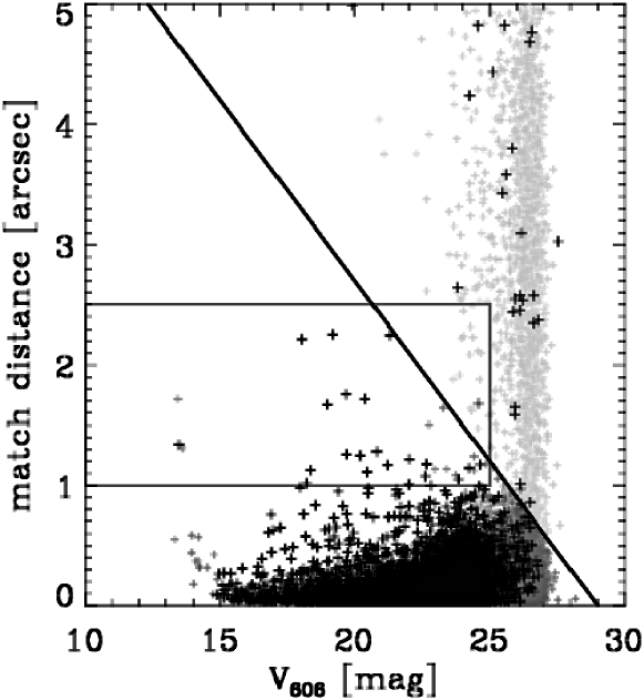
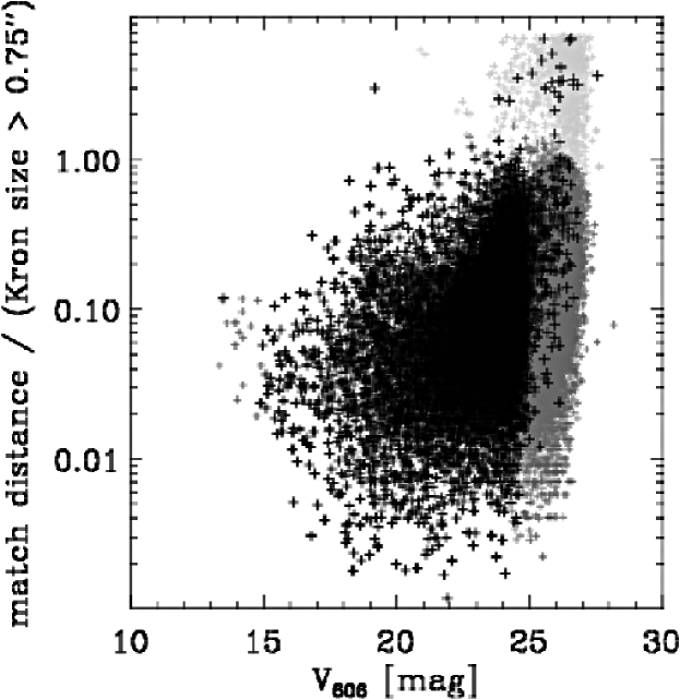
Figure 11: Cross-correlation of HST and COMBO-17 data. Left: The distance to the nearest neighbour within a search radius of 5″is plotted as a function of HST magnitude. At the faint end galaxies are matched to uncorrelated neighbours. Resolving irregular structures in the HST images results in detected galaxy centres being located farther from the COMBO-17 galaxy centre than a seeing distance. Matching bright objects at large separations while removing random correlations at faint fluxes requires a cut as indicated by the diagonal line. Objects within the box ($V_{606}<25$ and $1\arcsec<$ match distance $<2.5\arcsec$) were inspected by eye. Right: Ratio of matching distance and Kron size as a function of HST magnitude. Values larger than $\sim 1$ imply a matching radius larger than the object size in the HST image. Sources with $R_{\textrm{ap}}<24$ are shown as black symbols; objects with a match below the cut (diagonal line in left panel) are plotted in dark grey; the remaining sources with a match within 5″ are shown as light grey symbols.

In order to maximise the number of good matches between STAGES and COMBO-17, in particular at low redshift, i.e. A901/2 cluster distance, we have devised the following scheme. For STAGES the average source density corresponds to roughly two objects per 5″-radius circle. We cross-correlate the STAGES and COMBO-17 catalogues using a nearest neighbour matching algorithm as described above with a maximum matching radius of 5″. The resulting matches we plot in Fig. 11 (left panel). In particular at faint magnitudes many matches are found that appear unrelated. In contrast, at brighter magnitudes several sources are correlated at radii much larger than the COMBO-17 seeing (0.75″), which still identify the same object. In Fig. 11 we also show a line that subdivides the plot into two regions:

$$d_{m}=-0.3\times\left(V_{606}-29\right),$$ (7)

with the matching radius $d_{m}$ in arcsec and the STAGES SExtractor magnitude $V_{606}$. Below the line, objects are considered to be correlated, while above they are not correlated. This division is empirically motivated by the requirement to match objects at the faint end out to the COMBO-17 resolution limit (0.5″-1.0″) while also correlating sources at larger radii at the bright end. The slope of the curve was determined by visual inspection of the matches inside the indicated box. Typically, the distance between centroids is $\sim 0\aas@@fstack{\prime\prime}1$ (Fig. 12).

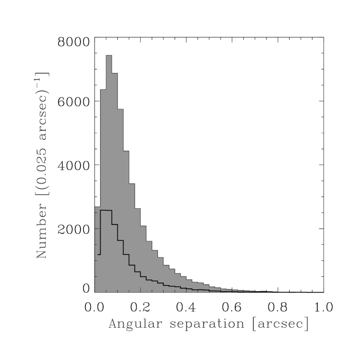
Figure 12: Histogram of matching radii for all objects (outer histogram) and $R_{\rm ap}<24$ objects (inner histogram). The typical angular separation between a COMBO-17 object with $R_{\textrm{ap}}<24$ and its HST counterpart is $\sim 0.12$″$\pm 0.08$″.

Another way of investigating this issue is by calculating whether the nearest matching neighbour falls within the area covered by the object in the STAGES image. If the projected COMBO-17 position is beyond the optical extent of the source in STAGES, it is uncorrelated. From the STAGES SExtractor data we estimate the ‘extent’ of an object by its Kron size $K=r_{\textrm{K}}\times a$, from the Kron radius $r_{\textrm{K}}$ and semi-major axis radius $a$. We limit the Kron size to $K>0.75$″. A ratio of $d_{m}/K\ga 1$ indicates that the matched COMBO-17 source lies outside the region covered by the object in the STAGES image. In Fig. 11 (right panel) we overplot in grey all sources that were assigned a partner from the nearest neighbour matching. This provides further evidence for the improved quality of our new cross-correlation method.

In summary, the combined catalogue contains 88 879 sources. Of these, $\sim 6\,577$ objects with a COMBO-17 ID are not within the region covered by the STAGES HST mosaic ($\sim 1\,664$ of these have $R_{\textrm{ap}}<24$). Moreover, $\sim 1\,271$ STAGES detections are outside the COMBO-17 observation footprint. Inside the region covered by both surveys, there are $\sim 81\,031$ sources. For 50701 objects the method described above provides a match between COMBO-17 and STAGES (15760 of these have $R_{\textrm{ap}}<24$). $\sim 23\,833$ sources detected in STAGES do not have counterparts in COMBO-17; $\sim 6\,497$ sources from the COMBO-17 catalogue are not matched to STAGES detections. Out of these, only $\sim 79$ objects have $R_{\textrm{ap}}<24$. We therefore emphasize that for our science sample of COMBO-17 objects, defined as having $R_{\textrm{ap}}<24$, 99.9% have a STAGES counterpart. The majority of failures result from confusion by neighbouring objects or simply non-detections.

3.3 Selection of an A901/2 cluster sample

We wish to define a ‘cluster’ galaxy sample of galaxies belonging to the A901/2 complex for various follow-up studies of our team that are in progress. These studies may have different requirements for the completeness of cluster members and the contamination by field galaxies. We therefore quantified how these two key values vary with both magnitude and width of the redshift interval in order to inform our choice of definition.

The photo-z distribution of cluster galaxies was assumed to follow a Gaussian with a width given by the photo-z scatter in Equation 5. The distribution of field galaxies was assumed to be consistent with the average galaxy counts $n(z,R)$ outside the cluster and varies smoothly with redshift and magnitude assuming no structure in the field. Samples were then defined by redshift intervals $z_{\rm phot}=[0.17-\Delta z,0.17+\Delta z]$, where the half-width $\Delta z$ was allowed to vary with the magnitude. We calculated completeness and contamination at all magnitude points simply using the counts of our smooth models.

We found that as long as the half-width in redshift is not much larger than a couple of Gaussian FWHMs, the contamination changes only little. The ratio of selected cluster to field galaxies is almost invariant as shrinking widths cut into numbers for both origins. Only enlarging the width significantly over that of the Gaussian increases contamination by field galaxies. On the contrary, such large widths do not affect the completeness of the cluster sample much, while shrinking the width too far eats into the true cluster distribution and reduces completeness of the cluster sample.

For our purposes, we compromised on a photo-z width such that the completeness is $>90$% at any magnitude, just before further widening starts to increase the contamination above its mag-dependent minimum (see Fig. 13 and Fig. 14, left panel). For this we chose a half-width of

$$\Delta z(R)=\sqrt{0.015^{2}+0.0096525^{2}(1+10^{0.6(R_{\rm tot}-20.5)})}~{}.$$ (8)

This equation defines a half-width that is limited to 0.015 at the bright end and expands as a constant multiple of the estimated photo-z error at the faint end. The floor of the half-width is motivated by including the entire cluster member sample previously studied by WMG05. The completeness of this selection converges to nearly 100% for bright galaxies, as a result of intentionally including the WGM05 sample entirely.

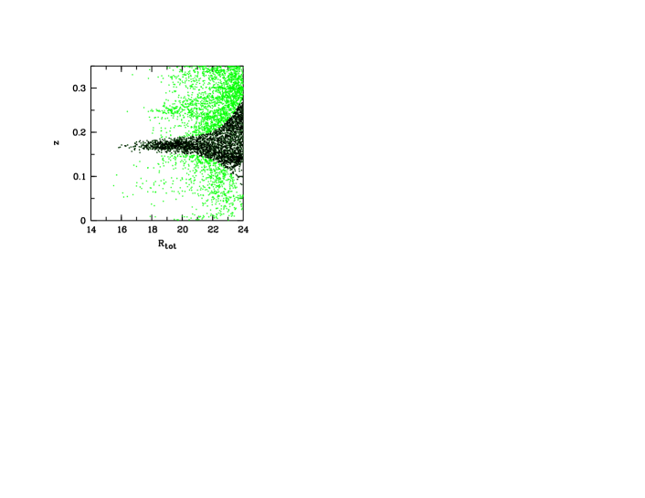
Figure 13: MEV redshift estimate vs. total $R$-band magnitude. The ’galaxy’ sample is shown in green, while the sample of ‘cluster’ galaxies defined by Equation 8 is shown in black. The magnitude-dependent redshift interval guarantees almost constant high completeness, while the field contamination increases towards faint levels (Fig. 14). We note that at faint magnitudes there is an apparent asymmetry towards lower redshift at faint magnitudes within the cluster sample. The photometric redshifts may be skewed by systematic effects but the average $-0.02$ offset at $R_{\rm tot}\sim 22.5$ is within the $1\sigma$ error envelope.

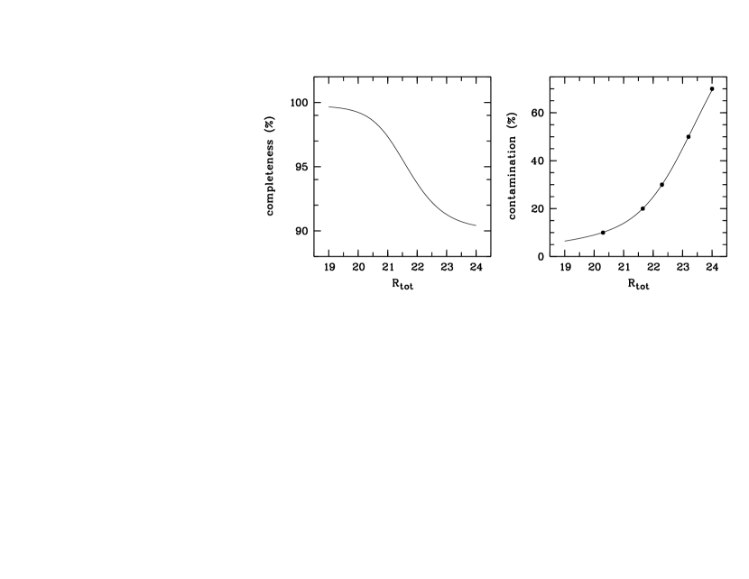
Figure 14: Left panel: Completeness of the cluster sample defined in Fig. 13 and designed to provide high completeness at all magnitudes. Right panel: The field contamination of the cluster sample increases at faint levels due to photo-z dilution of the cluster. Narrowing the selected redshift interval would not reduce the contamination. Contamination rates are estimated to be $(10,20,30,50,70)\%$ at $R_{\rm ap}=(20.3,21.65,22.3,23.2,24.0)$.

The right panel of Fig. 14 shows that the differential contamination increases rapidly towards faint magnitudes, simply as a result of the photo-z error-driven dilution of the cluster sample. Here, contamination means the fraction of galaxies that are field members, as measured in a bin centred on the given magnitude with width 0.1 mag. Contamination at a given apparent magnitude translates into contamination at a resulting luminosity at the cluster distance (except that scatter in the aperture correction smears out the contamination relation slightly).

Already at $R_{\it ap}=23.2$ the sample contains as many cluster as field members. This corresponds to $M_{V}\approx-16.5$ for the average galaxy, but scatters around that due to aperture corrections. As we probe fainter this selection adds more field galaxies than cluster members. Follow-up studies can now determine an individual magnitude or luminosity limit given their maximum tolerance for field contamination. For example, WGM05 selected cluster galaxies at $M_{V}-<-17.775$ ($M_{V}<-17$ for their adopted cosmology with $H_{0}=100$ km s^-1 Mpc^-1) for an earlier study of the A901/2 system in order to keep the contamination at the faint end below 20%.

The cluster sample thus obtained covers quite a range of photo-z values at the faint end, and restframe properties are derived assuming these redshifts to be correct. However, if we assume a priori that an object is at the redshift of the cluster, then we may want to know these properties assuming a fixed cluster redshift of $z=0.167$. Hence, the SED fits and restframe luminosities are recalculated for this redshift and reported in additional columns of the STAGES catalogue in Table 10 (with ‘_cl’ suffix indicating cluster redshift). Of course, if the a-priori assumption is to believe the redshifts as derived, then the original set of columns for which we have derived the values is relevant.

4 Further multiwavelength data and derived quantities

In this section we describe further multiwavelength data for the A901/2 region taken with other facilities (Fig. 2). We also present several resulting derived quantities (stellar masses and star formation rates) that appear as entries in the STAGES master catalogue.

4.1 Spitzer

Spitzer observed a $1\degr\times 0{\aas@@fstack{\circ}}5$ field around the A901/2 system in December 2004 and June 2005 as part of Spitzer GO-3294 (PI: Bell). The MIPS 24µm data were taken in slow scan-map mode, with individual exposures of 10 s. We reduced the individual image frames using a custom data-analysis tool (DAT) developed by the GTOs (Gordon et al., 2005). The reduced images were corrected for geometric distortion and combined to form full mosaics; the reduction which we currently use does not mask out asteroids and other transients in the mosaicing. The final mosaic has a pixel scale of $1\aas@@fstack{\prime\prime}25$ pixel^-1 and an image PSF FWHM of $\simeq 6$″. Source detection and photometry were performed using techniques described in Papovich et al. (2004); based on the analysis in that work, we estimate that our source detection is 80% complete at 97 $\mu$Jy for a total exposure of $\sim 1400$ s pix^-1. By detecting artificially-inserted sources in the A901 24 image, we estimated the completeness of the A901 24 $\mu$m catalog. The completeness is 80%, 50% and 30% at 5, 4 and 3$\sigma$, respectively.

Note that there is a very bright star at 24µm near the centre of the field at coordinates $(\alpha,\delta)_{\rm J2000}=(09^{h}56^{m}32\aas@@fstack{s}4,-10\degr 01\arcmin 15\arcsec)$ (see §A.1 for details of this object). In our analysis of the 24µm data we discard all detections less than 4^′ from this position in order to minimise contamination from spurious detections and problems with the background level in the wings of this bright star. It is to be noted that there are a number of spurious detections in the wings of the very brightest sources; while we endeavoured to minimise the incidence of these sources, they are difficult to completely eradicate without losing substantial numbers of real sources at the flux limit of the data.

To interpret the observed 24µm emission, we must match the 24µm sources to galaxies for which we have redshift estimates from COMBO-17. We adopt a 1″matching radius. In the areas of the A901/2 field where there is overlap between the COMBO-17 redshift data and the full-depth MIPS mosaic, there are a total of 3506(5545) 24µm sources with fluxes in excess of 97(58)$\mu$Jy. Roughly 62% of the 24µm sources with fluxes $>58\mu$Jy are detected by COMBO-17 in at least the deep $R$-band, with $R\la 26$. Some 50% of the 24µm sources have bright $R_{\rm tot}<24$ and have photometric redshift $z<1$; these 50% of sources contain nearly 60% of the total 24µm flux in objects brighter than 58$\mu$Jy. Sources fainter than $R\ga 24$ contain the rest of the $f_{24}>58\mu$Jy 24µm sources; investigation of COMBO-17 lower confidence photometric redshifts, their optical colours, and results from other studies lends weight to the argument that essentially all of these sources are at $z>0.8$, with the bulk lying at $z>1$ (e.g. Le Floc’h et al. 2004, Papovich et al. 2004; see Le Floc’h et al. 2005 for a further discussion of the completeness of redshift information in the CDFS COMBO-17 data).

Observations with IRAC (Infrared Array Camera; Fazio et al., 2004) at 3.6, 4.5, 5.8 and 8.0µm were also taken as part of this Spitzer campaign: those data are not discussed further here, and will be described in full in a future publication.

4.2 Star formation rates

We provide estimates of star formation rate, determined using a combination of 24µm data (to probe the obscured star formation) and COMBO-17 derived rest-frame 2800Å luminosities (to probe unobscured star formation). Ideally, we would have a measure of the total thermal IR flux from 8–1000µm; instead, we have an estimate of IR luminosity at one wavelength, 24µm, corresponding to rest-frame 22–12µm at the redshifts of interest $z=0.1-1$. Local IR-luminous galaxies show a tight correlation between rest-frame 12–15µm luminosity and total IR luminosity (e.g., Spinoglio et al., 1995; Chary & Elbaz, 2001; Roussel et al., 2001; Papovich & Bell, 2002), with a scatter of $\sim 0.15$ dex. Following Papovich & Bell (2002), we choose to construct total IR luminosity from the observed-frame 24µm data. We use the Sbc template from the Devriendt et al. (1999) SED library to translate observed-frame 24µm flux into the 8–1000µm total IR luminosity. The IR luminosity uncertainties are primarily systematic. Firstly, there is a natural diversity of IR spectral shapes at a given galaxy IR luminosity, stellar mass, etc.; one can crudely estimate the scale of this uncertainty by using the full range of templates from Devriendt et al. (1999), or by using templates from, e.g., Dale et al. (2001) instead. This uncertainty is $\la$0.3 dex (this agrees roughly with the scatter seen between 24µm luminosity and SFR seen in Calzetti et al., 2007). Secondly, it is possible that a significant fraction of $0.1<z<1.0$ galaxies have IR spectral energy distributions not represented in the local Universe: while it is impossible to quantify this error until the advent of Herschel Space Telescope, current results suggest that the bulk of intermediate–high redshift galaxies have IR spectra similar to galaxies in the local universe (Appleton et al., 2004; Elbaz et al., 2005; Yan et al., 2005; Zheng et al., 2007).

We estimate SFRs using the combined directly-observed UV light from young stars and the dust-reprocessed IR emission of the sample galaxies (e.g., Gordon et al., 2000). Following Bell et al. (2005), we estimate SFR $\psi$ using a calibration derived from PEGASE assuming a 100 Myr-old stellar population with constant SFR and a Chabrier (2003) IMF:

$$\psi/({\rm M_{\sun}\,yr^{-1}})=9.8\times 10^{-11}\times(L_{\rm IR}+2.2L_{\rm UV}),$$ (9)

where $L_{\rm IR}$ is the total IR luminosity (as estimated above) and $L_{\rm UV}=1.5\nu l_{\nu,2800}$ is a rough estimate of the total integrated 1216Å–3000Å UV luminosity, derived using the 2800Å rest-frame luminosity from COMBO-17 $l_{\nu,2800}$. The factor of 1.5 in the 2800Å-to-total UV conversion accounts for the UV spectral shape of a 100 Myr-old population with constant SFR, and the UV flux is multiplied by a factor of 2.2 before being added to the IR luminosity to account for light emitted longwards of 3000Å and shortwards of 1216Å by the unobscured young stars. This SFR calibration is derived using identical assumptions to Kennicutt (1998), and the calibration is consistent with his to within 30% once different IMFs are accounted for. Uncertainties in these SFR estimates are a factor of two or more in a galaxy-by-galaxy sense, and systematic uncertainty in the overall SFR scale is likely to be less than a factor of two (see, e.g., Bell, 2003; Bell et al., 2005, for further discussion of uncertainties). The adopted calibration assumes that the infrared luminosity traces the emission from young stars only; contributions from potential AGN can be identified and excluded by cross-matching with the X-ray and optical data as in Gilmour et al. (2007) and Gallazzi et al. (2008).

Again, for galaxies in the ‘cluster’ sample, we present also SFR estimates assuming that the galaxies are at the cluster redshift with the suffix ‘_cl’ in added to the column name.

4.3 Stellar Masses

Borch et al. (2006) estimated the stellar masses of galaxies in COMBO-17 using the 17-passband photometry in conjunction with a template library derived using the PEGASE stellar population model. The non-evolving template stellar populations had an age/metallicity combination equivalent to roughly solar metallicity and $\sim 6$ Gyr since the start of star formation. Borch et al. (2006) adopted a Kroupa et al. (1993) stellar IMF; the use of a Kroupa (2001) or Chabrier (2003) IMF would have yielded the same stellar masses to within $\sim 10$%. Such masses are quantitatively consistent with those derived using a simple colour-stellar M/L relation (Bell et al., 2003), and comparison of stellar and dynamical masses for a few $z\sim 1$ early-type galaxies yielded consistent results to within their combined errors (see Borch et al. 2006 for more details).

There are some galaxies for which the 17-band classification failed to find a satisfactory solution (2% of the galaxies with redshift estimates); we choose to adopt in these cases a rest-frame colour-derived stellar mass, using rest-frame $B$ and $V$ absolute magnitudes/luminosities, and a $V$-band absolute magnitude of the Sun of 4.82:

$$\log_{10}M_{*}/M_{\sun}=-0.728+1.305(B-V)+\log_{10}L_{V}/L_{\sun}.$$ (10)

As with restframe photometric properties, we also present estimates of stellar mass assuming that the galaxy is at the cluster redshift (denoted in the catalogues by the suffix ‘_cl’ in the column names). Random stellar mass errors are estimated to be $\sim 0.1$ dex on a galaxy-by-galaxy basis in most cases, and systematic errors in the stellar masses (setting the overall mass scale and its redshift evolution) were argued to be at the 0.1 dex level for galaxies without ongoing or recent major starbursts; for galaxies with strong bursts, masses could be overestimated by $\la 0.5$ dex.

Finally, we note potential aperture effects on stellar masses and SEDs for some objects. The colours are estimated within an aperture but are normalized by the total light in the deep $R$-band image alone. For small objects or particularly large objects without colour gradients this has no consequence. But if large size, low concentration and strong colour gradients are combined, the total SED will deviate from the aperture SED underlying the $M/L$ estimate. In a companion paper studying properties of spiral galaxies in the supercluster, Wolf et al. (MNRAS, accepted) have investigated this effect by examining the total colours across a wide parameter space in the sample. In most cases the aperture values are similar to the total ones, but they identify an issue for morphologically-classified spiral galaxies in the supercluster and eliminate the highest-mass regime with $\log M_{*}/M_{\sun}>11$ from their study.

4.4 GALEX

The Abell 901/902 field was observed by GALEX in the far-UV ($f,\lambda_{\rm eff}\sim 1528$Å) and near-UV ($n,\lambda_{\rm eff}\sim 2271$Å) bands. Individual observations (or single orbit ‘visits’) between the dates 12 February 2005 and 25 February 2007 were coadded by the GALEX pipeline (GR4 version Morrissey et al., 2007) to produce images with net exposure times of 57.18 ks in $n$ (47 visits) and 50.19 ks in $f$ (40 visits). The GALEX field of view in both bands is a 0.6°radius circle, and the average centre of the visits (the GALEX field centre) is $(\alpha,\delta)_{\rm J2000}=(9^{\rm h}56^{\rm m}20\aas@@fstack{s}7,-10\degr 6\arcmin 21\aas@@fstack{\prime\prime}6)$. The GALEX PSF near the field centre has $\sim 4.2$″ FWHM at $f$ and $\sim 5.3$″ FWHM at $n$, both of which increase with distance from the field centre (variations in the PSF that are not a function of distance from the field centre are smoothed out by the distribution of roll angles of the visits). The astrometric accuracy is $\sim 0.7$″, and $>97$% of catalogued source positions are within 2″ of their true positions. The photometric calibration is stable to $0.02$ mag in $n$ and $0.045$ mag in $f$ (Morrissey et al., 2007).

Source detection and photometry is via the GALEX pipeline code, which employs a version of SExtractor (Bertin & Arnouts, 1996) modified for use with low-background images. Magnitudes are measured both in fixed circular apertures and in automatic Kron elliptical apertures, and in isophotal apertures. The 5$\sigma$ point-source sensitivities in the Abell 901/902 field are $f\sim 24.7$ mag (AB) and $n\sim 25.0$ mag (AB), though there are spatial variations across field, especially a slightly decreasing sensitivity towards the edge of the field. At these levels source confusion in the $n$ band becomes an issue, and the $n$ band fluxes of faint objects ($n\ga 23$ mag) are likely to be overestimated. GALEX data products include intensity, background, and relative response (i.e., effective exposure time) maps in both bands as well as source catalogues in both bands and a band-merged source catalogue.

4.5 2dF spectroscopy

Spectra of cluster galaxies were obtained using the 2dF instrument on the AAT in March 2002 and March 2003. A total of 86 galaxies were observed using the 1200B grating (spanning the observed wavelength range 4000–5100 Å) in a single fibre configuration during the 2002 run. Three fibre configurations using the lower resolution 600V grating (spanning 3800–5800 Å) were observed during the 2003 run: fibres were placed on 368 objects, with 47 repeated from 2002. The primary selection function assigned higher priority to those galaxies selected by photometric redshift to be within the supercluster redshift slice and having $R<20$, with additional fibres being allocated to secondary targets (including fainter galaxies and a small number of white dwarfs and QSOs) when available. Data reduction was performed with the standard 2dfdr (v2.3) pipeline package.

In total, spectra were obtained for 407 unique objects. Redshifts were determined by two independent means: firstly by manual line profile fitting of the Ca H and K features in absorption and secondly by cross-correlation with template spectra using the XCSAO task within IRAF (Kurtz & Mink 1998). Comparison of the two measurements showed no cause for concern, with $\Delta_{z}=0.00149\pm 0.00006$. After eliminating non-galaxy and poor quality spectra, we have redshifts for 353 galaxies in total.

The 2dF spectroscopic data have previously been used to quantify the reliability of the COMBO-17 redshifts in W04 (see also §3), to verify cluster membership for the matched X-ray point sources (Gilmour et al., 2007), and to create composite spectra for three photometric classes of cluster galaxies in WGM05. A dynamical analysis of the the clusters using the 2dF redshifts will be presented in Gray et al. (in prep.).

4.6 XMM-Newton

X-ray data for the A901/2 region is desirous both to detect point-source emission from cluster members (star-formation or AGN) and the extended intracluster medium (ICM). A 90 ks XMM image of the A901/2 field was taken on May 6/7 2003 using the three EPIC cameras (MOS1, MOS2 and PN) and a thin filter, under program 14817 (PI: Gray). The level 1 data were taken from the supplied pipeline products, and reduced with SAS v5.4 and the calibration files available in May 2003. Final exposure times were $\sim 67$ ks for MOS and $\sim$61 ks for PN following the removal of time intervals suffering from soft proton flares. Four energy bands were used: 0.5-2 keV (soft band), 2-4.5 keV (medium band), 4.5-7.5 keV (hard band) and 0.5-7.5 keV (full band).

The creation of the point-source catalogue using wavelet detection methods is described in detail elsewhere (Gilmour et al., 2007). A total of 139 significant sources were found. The presence of an X-ray luminous Type-I AGN near the centre of A901a (see Appendix A.3) complicated the detection of the underlying extended cluster emission. A maximum-likelihood technique was used to match this catalogue to COMBO-17 resulting in 66 secure counterparts with photometric redshifts. Gilmour et al. (2007) used these data to examine the local environments of the cluster AGN and their host properties.

To isolate the remaining extended emission coming from the clusters, a separate conservative point-source catalogue was constructed. Care was taken to remove both the cosmic background and spatial variations in the non-cosmic background. The background subtracted images were weighted by appropriate energy conversion factors to create flux images for each detector. These flux images were masked and summed together to create merged background-subtracted images in each band.

Point source regions were removed and replaced with the local background value selected randomly from a source free area within 10 pixels (or 20 pixels if there were not enough background pixels within the smaller radius). Smoothed images were created in each band using a Gaussian kernel of radius 4 pixels. Maps of the extended emission and an examination of the global X-ray properties of the clusters will be presented in Gray et al. (in prep.).

4.7 GMRT

The A901/2 field was observed on 2007 March 25th and 26th March with the Giant Metrewave Radio Telescope (GMRT, see Ananthakrishnan 2005 for further details). The field was centred at $(\alpha,\delta)_{\rm J2000}=(09^{\rm h}56^{\rm m}17^{\rm s},-10\degr 01\arcmin 28\arcsec)$ and observed at 610 and 1280 MHz on respective nights. The GMRT is an interferometer, consisting of thirty antennas, each 45 m in diameter. The bright sources 3C147 and 3C286 were observed at the start and end of each observing session, in order to set the flux density scale. During the observations a nearby compact source 0943$-$083 was observed for about 4 minutes at roughly 30 minutes intervals, to monitor and correct any antenna-based amplitude and phase variations.

The total integration time on the field was $\sim$6.5 hours at each frequency. The observations covered two 16 MHz sidebands, positioned above and below the central frequency. Each sideband was observed with 128 narrow channels, in order to allow narrow band interference to be identified and efficiently removed. The observed visibility data were edited and calibrated using standard tasks with the AIPS package, and then groups of ten adjacent channels were averaged together, with some end channels discarded. This reduced the volume of the visibility data, whilst retaining enough channels so that chromatic aberration is not a problem (e.g., see Garn et al., 2007, for further details of GMRT analysis). Given the relatively large field of view of the GMRT compared with its resolution, imaging in AIPS requires several ‘facets’ to be imaged simultaneously, and then be combined. Preliminary imaging results, after several iterations of self-calibration, have produced images with resolutions of about 5″and 2$\aas@@fstack{\prime\prime}$5 at 610 and 1280-MHz respectively, with r.m.s. noises of approximately 25 and 20 $\mu$Jy beam^-1 in the centre of the fields, before correction for the primary beam of the GMRT. The primary beam – i.e. the decreasing sensitivity away from the field centres due to sensitivity of individual 45-m antennas – is approximately Gaussian, with a half-power beam width (HPBW) of approximately 44′and 26′at 610 and 1280-MHz respectively. These images are among the deepest images made at these frequencies with the GMRT. Further analysis and the source catalogue will be presented in Green et al.(in prep.).

4.8 Simulations and mock galaxy catalogues

In order to facilitate the interpretation of the observational results and to study the physical processes of galaxy evolution, N-body, hydrodynamic, and semi-analytic simulations that closely mimic the A901/2 system are being produced (van Kampen et al., in prep.). We constrain initial conditions using the method of Hoffman & Ribak (1991) to take into account the gross properties of A901a, A901b, A902, the SW group, and the neighbouring clusters A868 and A907 (outside the observed field). The simulations produce a range of mock large-scale structures to test three basic formation scenarios: a ’stationary’ case, where A901(a,b) and A902 will not merge within a Hubble time, and a pre- as well as a post-merger scenario. When the likelihood of each scenario is understood, one can further test the models for the detailed physical processes known to be operating on galaxies in and around such clusters.

5 Summary and Data Access

We have presented the multiwavelength data available for the A901/2 supercluster field as part of the STAGES survey: high-resolution HST imaging over a wide area, extensive photometric redshifts from COMBO-17, and further multiwavelength observations from X-ray to radio. These data have already been used to create a high resolution mass map of the system using weak gravitational lensing (Heymans et al., 2008). Further work by the STAGES team to study galaxy evolution and environment is ongoing and includes the following:

• Gallazzi et al. (2008) explore the amount of obscured star-formation as a function of environment in the A901/2 supercluster and associated field sample by combining the UV/optical SED from COMBO-17 with the Spitzer 24$\mu$m photometry in galaxies with $M_{*}>10^{10}M_{\sun}$. Results indicate that while there is an overall suppression in the fraction of star-forming galaxies with density, the small amount of star formation surviving the cluster environment is to a large extent obscured.

• Wolf et al. (MNRAS, accepted) investigate the properties of optically passive spiral and dusty red galaxies in the supercluster and find that the two samples are largely equivalent. These galaxies form stars at a substantial rate that is only a factor of four times lower than blue spirals at fixed mass, but their star formation is more obscured and has weak optical signatures. They constitute over half of the star forming galaxies at masses above $\log M_{*}/M_{\sun}=10$ and are thus a vital ingredient for understanding the overall picture of star-formation quenching in cluster environments.

• Marinova et al. (ApJ, submitted) identify and characterize bars in bright ($M_{V}\leq-18$) cluster galaxies through ellipse-fitting. The selection of moderately inclined disk galaxies via three commonly used methods, visual classification, colour, and Sérsic cuts, shows that the latter two methods fail to pick up many red, bulge-dominated disk galaxies in the clusters. However, all three methods of disk selection yields a similar global optical bar fractions ($f_{\rm bar-opt}\sim 0.3)$, averaged over all galaxy types. When host galaxy properties are considered, the optical bar fraction is found to be a strong function of both the luminosity and morphological property (bulge-to-disk ratio) of the host galaxy, similar to trends recently reported in field galaxies. Furthermore, results indicate that the global optical bar fraction for bright galaxies is not a strong function of local environment.

• Heiderman et al. (in prep.) identify interacting galaxies in the supercluster using quantitative analysis and visual classifications. Their findings include that $4.9\pm 1.3\%$ of bright ($M_{V}\leq-18$), intermediate mass ($M_{*}\geq 1\times 10^{9}M_{\sun}$) galaxies are interacting. The interacting galaxies are found to lie outside the cluster cores and to be concentrated in the region between the cores and virial radii of the clusters. Explanations for the observed distribution include the large galaxy velocity dispersion in the cluster cores and the possibility that the outer parts of the clusters are accreting groups, which are predicted to show a high probability for mergers and strong interactions. The average star formation rate is enhanced only by a modest factor in interacting galaxies compared to non-interacting galaxies, similar to conclusions reported in the field by Jogee et al. (2008). Interacting galaxies only contribute $\sim$ 20% of the total SFR density in the A901/902 clusters.

• Boehm et al. (in prep.) are utilizing the stability of the PSF on the STAGES images for a morphological comparison between the hosts of  20 type-1 AGN and  200 inactive galaxies at an average redshift $\left<z\right>\sim 0.7$. This analysis includes extensive simulations of the impact of a bright optical nucleus on quantitative galaxy morphologies in terms of the CAS indices and Gini/$M_{20}$ space. We find that the majority of the hosts cover parameters typical for disk+bulge systems and mildly disturbed galaxies, while evidence for strong gravitational interactions is scarce.

• Bacon et al. (in prep.) are examining the higher order lensing properties of the STAGES data. They construct a shapelets catalogue (Refregier, 2003) for the STAGES galaxies; this is then used to estimate the gravitational flexion (Bacon et al., 2006) at each galaxy position. Galaxy–galaxy flexion is measured, leading to estimates of concentration and mass for STAGES galaxies; constraints on cosmic flexion are also found, showing very good containment of systematic effects. The ability of flexion to improve convergence maps is also discussed.

• Robaina et al. (in prep.) make use of a combined GEMS and STAGES sample of $0.4<z<0.8$ galaxies to find that interacting and merging close pairs of massive galaxies ($>10^{10}M_{\odot}$) show a modest enhancement of their star formation rate; in particular, less than 15% of star formation at $0.4<z<0.8$ is triggered by major interactions and mergers.

• Barden et al. (in prep.) are exploring both the GEMS and STAGES data sets to investigate the evolution of structural parameters of disc galaxies as a function of luminosity and stellar mass over a wide range of environments and morphologies. In the process, GALAPAGOS will be extended to perform bulge/disc decomposition.

• McIntosh et al. (in prep.) are using both quantitative and qualitative morphologies to explore the morphological mix of red sequence galaxies as a function of stellar mass over the last seven billion years from the combined STAGES + GEMS sample.

It is our intention that the data products described here should be publicly available for use by the wider community for those interested in the supercluster itself or for data-mining the entire survey volume. To that end, the reduced HST images (both tiles and individual galaxy postage stamps) are available for download at the Multimission Archive at Space Telescope (MAST). Furthermore, the complete STAGES catalogue described in this paper is available from the STAGES website, including all HST-derived parameters; GALFIT profile fitting results; COMBO-17 photometry, SEDs and photometric redshifts; and stellar masses and star-formation rates. The multiwavelength data available there includes the Spitzer/MIPS 24µm images and catalogue; the X-ray point source catalogue (Gilmour et al., 2007) and the gravitational lensing mass maps (Heymans et al., 2008). GALEX data and catalogues are available via MAST. The X-ray maps, 2dF spectra and radio catalogue and mocks will be also be placed on the website with the publication of their associated papers, or may be made available upon request. Table 9 contains a summary of the available data products.

Table 9: Description of all available A901/902 data products.

Data product	Date of release	Reference
HST F606W imaging, reduced: tiles, thumbnails, colour jpegs	immediate	this paper
STAGES master catalogue: SExtractor, GALFIT, COMBO-17, stellar masses, SFRs	immediate	this paper
COMBO-17 SEDS and completeness tables	immediate	this paper
GALFIT profile fitting completeness from simulations	immediate	this paper
Spitzer 24µm imaging and catalogue	immediate	this paper
HST-derived weak lensing mass map	immediate	Heymans et al 2008
XMM point source catalogue	immediate	Gilmour et al 2007
GALEX imaging and catalogues (from the GALEX archive)	immediate	this paper
X-ray imaging	on request	Gray et al. (in prep.)
2dF spectroscopy	on request	Gray et al. (in prep.)
GMRT catalogue	TBC	Green et al. (in prep.)
constrained simulations and mock galaxy catalogues	TBC	van Kampen et al. (in prep.)

6 Acknowledgements

The STAGES team would like to thank Hans-Walter Rix for his crucial support in bringing this project to fruition. We also thank Alfonso Aragón-Salamanca, Anna Gallazzi, Amanda Heiderman, Irina Marinova, and Aday Robaina for their work in exploiting the STAGES dataset. Support for STAGES was provided by NASA through GO-10395 from STScI operated by AURA under NAS5-26555. MEG and CW were supported by STFC Advanced Fellowships. CH acknowledges the support of a European Commission Programme 6th framework Marie Cure Outgoing International Fellowship under contract MOIF-CT- 2006-21891. CYP was supported by the NRC-HIA Plaskett Fellowship, and the STScI Institute/Giacconi Fellowship. EFB and KJ are grateful for support from the DFG’s Emmy Noether Programme of the Deutsche Forschungsgemeinschaft, AB by the DLR (50 OR 0404), MB and EvK by the Austrian Science Foundation FWF under grant P18416, SFS by the Spanish MEC grants AYA2005-09413-C02-02 and the PAI of the Junta de Andaluc´a as research group FQM322, SJ by NASA under LTSA Grant NAG5-13063 and NSF under AST-0607748 and DHM by NASA under LTSA Grant NAG5-13102.

Appendix A Notes on individual objects

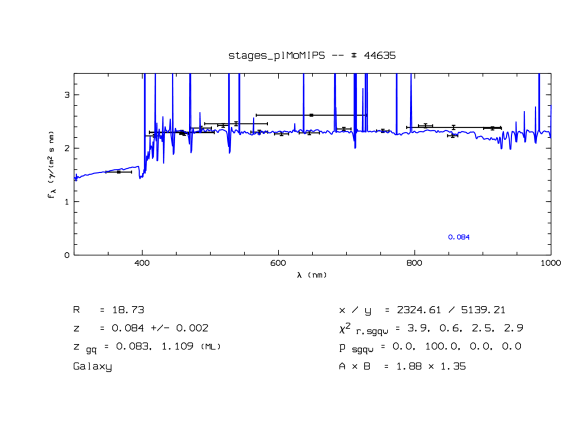
Figure 15: The COMBO-17 SEDs of the merging system 44635 (top) and 45154 (bottom). The latter case is a dust-reddened fit by eye to $z=0.08$, the likely redshift of the system.

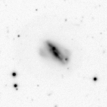
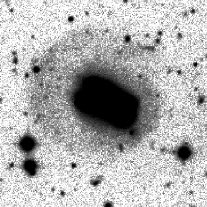
Figure 16: Left panel: The 20 ks COMBO-17 $R$-band image of the merging system that is with $\sim 50$ mJy the brightest extragalactic 24$\mu$ source in the field (objects 44635 and 45154, size of image $1\arcmin\times 1\arcmin$, N is up, E is left) and missing from the matched catalogue. Right panel: The same image in hard cuts reveals a tidal arm with 1/5000th of the surface brightness of the central disks. This arm is too faint to be visible in the STAGES/HST images.

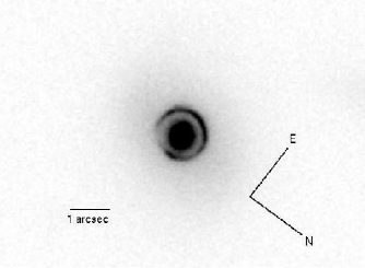
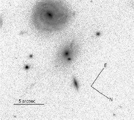
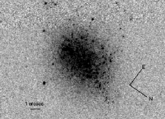
Figure 17: Left: The Einstein ring on an S0 cluster member. Centre: The cD galaxy in CB I at $z\approx 0.47$ is the central object, while the bright spiral to the upper left is a member of A902. Right: The nearby dwarf irregular STAGES I.

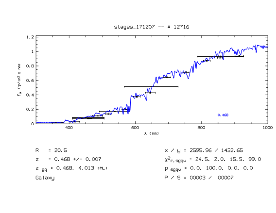
Figure 18: The COMBO-17 SED of object 12716, the central dominating (cD) galaxy of CB I, the cluster at $z\approx 0.47$ in the background of A902.

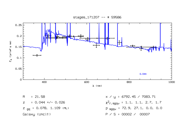
Figure 19: The COMBO-17 SED of STAGES I (object 59586), a dwarf irregular at $z_{\rm phot}\approx 0.04$ (but likely $z<0.01$).

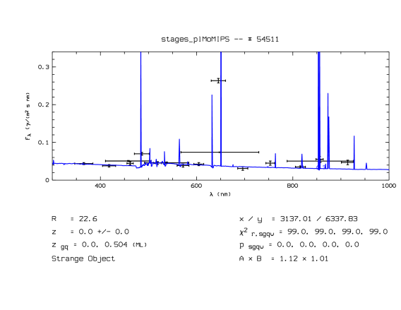
Figure 20: The COMBO-17 SED of the only photometrically-classified ‘strange’ object in the dataset: galaxy 54511 is at $z\approx 0.3$ and has extremely strong emission lines (OIII+H$\beta$ with $EW\approx 150$ nm).

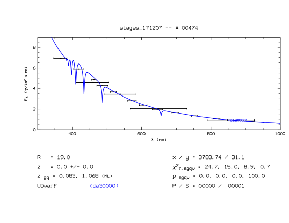
Figure 21: The COMBO-17 SED of object 474, the bluest white dwarf in the field. The lack of H$\beta$ absorption (see 485 filter) makes it a DB white dwarf. The best-fitting temperature is $\sim 30,000$ K.

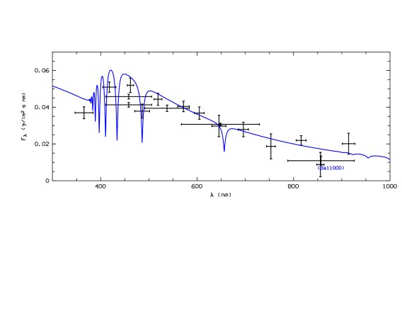
Figure 22: The COMBO-17 SED of object 33783, the faintest white dwarf in the field. The strong H$\beta$ absorption line in the 485 filter allows its classification even at this faint level ($R=23.4$, $T_{\rm eff}\approx 11,000$ K).

Here, we collect some details on ten noteworthy individual objects that have either extreme properties or are intrinsically rare and found only by chance in a field of this size. They are drawn from the COMBO-17 sample and are identified here via their COMBO-17 object numbers.

A.1 The brightest near-infrared source: a Mira variable

The object with the COMBO-17 number 35250 is classified as a very red star of spectral type M8 III in the 13th General Catalogue of MK Spectral Classifications (Buscombe, 1998). It is also known as the IRAS point source $09540-0946$, located at $(\alpha,\delta)_{\rm J2000}=(09^{h}56^{m}32\aas@@fstack{s}4,-10\degr 01\arcmin 15\arcsec)$, and it is a ROSAT All-Sky Survey Bright source (Voges et al., 1999). It has a very red SED with $(B,R,J,K)\approx(16,13.3,7.25,5.75)$ and is the brightest object in the field at $\lambda>1~{}\micron$. However, it has a large variability amplitude and was identified as a long-period pulsating Mira star in a search for high-redshift QSOs (Kirkpatrick et al., 1997). The area around this object had to be excluded from the Spitzer IRAC imaging due to its high brightness.

A.2 The brightest far-infrared galaxy: a merger

The brightest 24$\micron$ galaxy is a system of two merging disk galaxies with a total magnitude of $R\approx 16$. The Northern system (44635) has a very blue SED $(U-V)_{\rm rest}=0.14$ and implies a very strong H$\alpha$ line given its elevated $R$-band flux (see Fig. 15). The Southern system (45154) has an extremely red SED $(U-V)_{\rm rest}=1.97$ and implies strong dust-reddening. Their reshifts are estimated as $z_{\rm phot}=0.084$ and $0.053$, but the blue SED is better constrained by emission lines. Assuming $z=0.08$ for both objects, the projected separation between their two nuclei of $3\aas@@fstack{\prime\prime}5$ translates into 5 kpc.

The 20 ks $R$-band image of COMBO-17 shows tidal features with very low surface brightness (Fig. 16). The arm that reaches once around the entire galaxy has 5000$\times$ lower surface brightness than the main disks of the two merging galaxies. The system is also a strong radio source (NVSS J095643-095544) and was seen by IRAS. In our Spitzer MIPS images it shows $\sim 50$ mJy of flux, but such bright FIR measurements are missing from our matched catalogue due to matching difficulties. Preliminary analysis of the GMRT data reveals a strong radio detection at both 1280 MHz and 610 MHz with total flux S(1280)=$5.63\pm 0.05$ mJy/bm and S(610)=$13.68\pm 0.05$ mJy. The radio souce is partially resolved with a deconvolved size of $4.5\arcsec\times 1.9\arcsec$ at 1280 MHz and $4.1\arcsec\times 1.9\arcsec$ at 610 MHz, and a position angle of 40°at both frequencies.

A.3 The brightest X-ray source: a type-I AGN in A901a

Object 41435 is a massive red-sequence elliptical with excess blue light in its SED (see Fig. 7 of Gilmour et al., 2007) that has biased the redshift estimation. While it has $z_{\rm phot}\approx 0.33$, it is almost certainly a cluster member and a $z=0.16$ template fitted by hand works well and leaves over some room for AGN light. It is the brightest X-ray source in the STAGES field observed by XMM and a point source with a luminosity (assuming $z=0.16$) of $L_{X}=1.55\times 10^{44}$ erg/s. It is also the brightest radio source at 1280 MHz and is unresolved with total flux $46.33\pm 0.01$ mJy/bm. At 610 MHz it is partially resolved with an integrated flux density of $171.3\pm 0.1$ mJy.

A.4 An S0 galaxy with a full Einstein ring

Object 14049 (Fig. 17, left) is an S0 galaxy displaying a full optical Einstein ring. It has $z_{\rm phot}=0.23$, but 2dF spectroscopy confirms it is a cluster member with $z_{\rm spec}=0.168$, implying that the SED is contaminated by light from the lensed galaxy. Subsequent targetted spectroscopy revealed a source redshift $z_{s}=1.5$ (Aragón-Salamanca et al, in prep.).

A.5 A galaxy cluster in projection behind A902: CBI

Examination of the redshift distribution along the line-of-sight to the A902 cluster revealed the presence of a massive background cluster at $z\sim 0.47$, subsequently designated CBI (Fig. 17, centre). A 3D lensing approach (Taylor et al., 2004) was used to constrain the masses of the two clusters beyond the 2D mass reconstruction of Gray et al. (2002). Object 12716 ($R=19.1$) is the central cD galaxy of CBI and is detected as an unresolved object in the preliminary analysis of the GMRT data with $S_{\rm int}(1280\rm{MHz})=2.07\pm 0.02$mJy/bm and $S_{\rm int}(610\rm{MHz})=6.70\pm 0.04$ mJy. Its brighter and bluer close neighbour ($R=17.8$) is an actual member of A902 (see Fig. 17, centre).

A.6 The dwarf irregular galaxy STAGES I

The object with the COMBO-17 number 59586 is a nearby dwarf irregular galaxy (see Fig. 17, right and Fig. 19) estimated at $z_{\rm phot}=0.044\pm 0.026$ (consistent with $z=0$ at 1.6$\sigma$). At the estimated redshift it would have $M_{V}\approx-16.7$ and $\log M_{*}/M_{\odot}\approx 8.7$; however given the brightness of the resolved point sources it is most likely at $z<0.01$. It has a Sérsic index of $n=0.55$ and shows clear signs of irregularity besides a blue colour.

A.7 The galaxy with the strongest emission lines

The COMBO-17 catalogue contains only one object classified as ‘strange’ as a result of having a $\chi^{2}_{\rm red}>30$ for its best template fit, while having good flags: object 54511 is a galaxy with extremely strong emission lines and $R\approx 22.5$. The emission-line flux in the $R$-band and the 646-band both suggest $EW\approx 150$ nm, which would need to be the combined H$\beta$ and OIII lines. A line in the filter 485/30 shows $EW\approx 14$ nm and is possibly OII. The redshift of the object appears to be constrained to $0.27<z_{\rm lines}<0.32$ by a third line signal in the filter 855 (H$\alpha$; see Fig. 20).

A.8 The bluest white dwarf: $U-B<-1$

Object 474 is the bluest white dwarf with a satisfying fit to our DA template library, although the SED (see Fig. 21) shows clearly no H$\beta$ absorption line, rendering this object a DB. The best-fitting temperature is $\sim 30,000$ K.

A.9 The faintest white dwarf we could identify

Object number 33783 is the faintest white dwarf our classification can identify with $U=23.3$ and $R=23.4$. At this magnitude level, the WD selection is already highly incomplete, but the strong H$\beta$ absorption still constrains the template fit (see Fig. 22).

Appendix B STAGES master catalogue

The tables in this section contain information relating to the publically-available STAGES master catalogue. Table 10 lists and defines the column names containing STAGES and COMBO-17 data and derived stellar masses and star-formation rates. Table 12 details the three sample flags in the catalogue and describes how they are to be used to select relevant populations from the overlap between the HST, COMBO-17, and Spitzer datasets.

Table 10: Column entries in the published FITS catalogue, their headers and meanings. Some restframe luminosities are extrapolated in some redshift ranges. We give the redshift intervals, where no extrapolation errors are expected.

STAGES information
st_number	object number
st_x_image	x-position from SExtr in [pix] on tile
st_y_image	y-position from SExtr in [pix] on tile
st_cxx_image	ellipse parameter from SExtr in [pix]
st_cyy_image	ellipse parameter from SExtr in [pix]
st_cxy_image	ellipse parameter from SExtr in [pix]
st_theta_image	pos. angle from SExtr in [deg] in image
	coordinates (measured from right to up)
st_theta_world	pos. angle in [deg] in world coordinates
st_ellipticity	ellipticity from SExtr
st_kron_radius	Kron radius in units of [st_a_image]
st_a_image	semi-major half-axis from SExtr in [pix]
st_b_image	semi-minor half-axis from SExtr in [pix]
st_alpha_J2000	right ascension from SExtr in [deg]
st_delta_J2000	declination from SExtr in [deg]
st_ background	background value from SExtr in [counts]
st_flux_best	“best” flux from SExtr in [counts]
st_fluxerr_best	error of st_flux_best
st_mag_best	“best” magnitude from SExtr in [AB mag]
st_magerr_best	error of st_mag_best
st_flux_radius	half-light radius from SExtr in [pix]
st_isoarea_image	isophotal area from SExtr in [pix2]
st_fwhm_image	FWHM from SExtr in [pix]
st_flags	SExtr quality flags
st_class_star	SExtr stellarity estimator
st_org_image	postage stamp image file name
st_file_galfit	GALFIT output filename containing fit data
st_X_galfit	x-position on postage stamp in [pix]
st_Xerr_galfit	error of st_X_galfit
st_Y_galfit	y-position from GALFIT in [pix]
st_Yerr_galfit	error of st_Y_galfit
st_MAG_galfit	total magnitude from GALFIT in [AB mag]
st_MAGerr_galfit	error of st_MAG_galfit
st_RE_galfit	half-light radius from GALFIT in [pix]
st_REerr_galfit	error of st_RE_galfit
st_N_galfit	Sérsic index from GALFIT
st_Nerr_galfit	error of st_N_galfit
st_Q_galfit	major-to-minor axis ratio from GALFIT
st_Qerr_galfit	error of st_Q_galfit
st_PA_galfit	pos. angle in [deg] measured from up to left
st_PAerr_galfit	error of st_PA_galfit
st_sky_galfit	sky value from GALAPAGOS
st_tile	tile number in STAGES mosaic
COMBO-17 general information
COMBO_nr	COMBO-17 A901/2 field object number
ra	right ascension (J2000)
dec	declination (J2000)
xpix	x-position on COMBO-17 $R$-frame in pixels
ypix	y-position on COMBO-17 $R$-frame in pixels
Rmag	total $R$-band magnitude
e_Rmag	1-$\sigma$ error of total $R$-band mag
ap_Rmag	aperture $R$-band magnitude in run E
apd_Rmag	difference total to aperture (point source $\sim 0$)
Various flags for sample selection
phot_flag	COMBO-17 photometry flags (see Sect. 3.5)
combo_flag	COMBO-17 sample flag (see Table 12)
stages_flag	STAGES sample flag (see Table 12)
mips_flag	MIPS sample flag (see Table 12)

COMBO-17 classification results
chi2red	$\chi^{2}/N_{f}$ of best-fitting template
chi2reds	$\chi^{2}/N_{f}$ of best-fitting star template
chi2redg	$\chi^{2}/N_{f}$ of best-fitting galaxy template
chi2redq	$\chi^{2}/N_{f}$ of best-fitting QSO template
chi2redw	$\chi^{2}/N_{f}$ of best-fitting WD template
chi2redg_cl	$\chi^{2}/N_{f}$ of best-fitting galaxy template at $z=0.167$
mc_class	multi-colour class (see Table 7)
mc_z	mean redshift in distribution $p(z)$
e_mc_z	standard deviation (1-$\sigma$) in distribution $p(z)$
mc_z2	alternative redshift if $p(z)$ bimodal
e_mc_z2	standard deviation (1-$\sigma$) at alternative redshift
mc_z_ml	peak redshift in distribution $p(z)$
mc_Ebmv	mean $E(B-V)$ in distribution $p(z)$
e_mc_Ebmv	standard deviation (1-$\sigma$) in distribution $p($E(B-V)$)$
mc_Ebmv_ml	peak value in distribution $p(E(B-V))$
mc_age	mean template age index
e_mc_age	standard deviation (1-$\sigma$) of template age index
mc_age_ml	peak in template age index distribution
mc_z_cl	redshift assuming cluster membership
mc_Ebmv_cl	mean $E(B-V)$ assuming cluster membership
e_mc_Ebmv_cl	standard deviation in $p(E(B-V))$ if cluster member
mc_age_cl	mean age index assuming cluster membership
e_mc_age_cl	standard deviation in age index if cluster member
total galaxy restframe luminosities
S280Mag	$M_{\rm abs,gal}$ in 280/40 ($z\approx[0.25,1.3]$)
e_S280Mag	1-$\sigma$ error of $M_{\rm abs,gal}$ in 280/40
UjMag	$M_{\rm abs,gal}$ in Johnson $U$ (ok at all $z$)
e_UjMag	1-$\sigma$ error of $M_{\rm abs,gal}$ in Johnson $U$
BjMag	$M_{\rm abs,gal}$ in Johnson $B$ ($z\approx[0.0,1.1]$)
e_BjMag	1-$\sigma$ error of $M_{\rm abs,gal}$ in Johnson $B$
VjMag	$M_{\rm abs,gal}$ in Johnson $V$ ($z\approx[0.0,0.7]$)
e_VjMag	1-$\sigma$ error of $M_{\rm abs,gal}$ in Johnson $V$
usMag	$M_{\rm abs,gal}$ in SDSS $u$ (ok at all $z$)
e_usMag	1-$\sigma$ error of $M_{\rm abs,gal}$ in SDSS $u$
gsMag	$M_{\rm abs,gal}$ in SDSS $g$ ($z\approx[0.0,1.0]$)
e_gsMag	1-$\sigma$ error of $M_{\rm abs,gal}$ in SDSS $g$
rsMag	$M_{\rm abs,gal}$ in SDSS $r$ ($z\approx[0.0,0.5]$)
e_rsMag	1-$\sigma$ error of $M_{\rm abs,gal}$ in SDSS $r$
restframe luminosities at cluster distance
S280Mag_cl	$M_{\rm abs,gal}$ in 280/40 (if cluster member)
e_S280Mag_cl	1-$\sigma$ error of $M_{\rm abs,gal}$ in 280/40
UjMag_cl	$M_{\rm abs,gal}$ in Johnson $U$ (if cluster member)
e_UjMag_cl	1-$\sigma$ error of $M_{\rm abs,gal}$ in Johnson $U$
BjMag_cl	$M_{\rm abs,gal}$ in Johnson $B$ (if cluster member)
e_BjMag_cl	1-$\sigma$ error of $M_{\rm abs,gal}$ in Johnson $B$
VjMag_cl	$M_{\rm abs,gal}$ in Johnson $V$ (if cluster member)
e_VjMag_cl	1-$\sigma$ error of $M_{\rm abs,gal}$ in Johnson $V$
usMag_cl	$M_{\rm abs,gal}$ in SDSS $u$ (if cluster member)
e_usMag_cl	1-$\sigma$ error of $M_{\rm abs,gal}$ in SDSS $u$
gsMag_cl	$M_{\rm abs,gal}$ in SDSS $g$ (if cluster member)
e_gsMag_cl	1-$\sigma$ error of $M_{\rm abs,gal}$ in SDSS $g$
rsMag_cl	$M_{\rm abs,gal}$ in SDSS $r$ (if cluster member)
e_rsMag_cl	1-$\sigma$ error of $M_{\rm abs,gal}$ in SDSS $r$
QSO restframe luminosities
S145Mag	$M_{\rm abs,QSO}$ in 145/10 ($z\approx[1.4,5.2]$)
e_S145Mag	1-$\sigma$ error of $M_{\rm abs,QSO}$ in 145/10

Table 11: continued

observed seeing-adaptive aperture fluxes
W420f	photon flux in filter 420
e_W420f	1-$\sigma$ photon flux error in 420
W462f	photon flux in filter 462
e_W462f	1-$\sigma$ photon flux error in 462
W485f	photon flux in filter 485
e_W485f	1-$\sigma$ photon flux error in 485
W518f	photon flux in filter 518
e_W518f	1-$\sigma$ photon flux error in 518
W571f	photon flux in filter 571
e_W571f	1-$\sigma$ photon flux error in 571
W604f	photon flux in filter 604
e_W604f	1-$\sigma$ photon flux error in 604
W646f	photon flux in filter 646
e_W646f	1-$\sigma$ photon flux error in 646
W696f	photon flux in filter 696
e_W696f	1-$\sigma$ photon flux error in 696
W753f	photon flux in filter 753
e_W753f	1-$\sigma$ photon flux error in 753
W815f	photon flux in filter 815
e_W815f	1-$\sigma$ photon flux error in 815
W856f	photon flux in filter 856
e_W856f	1-$\sigma$ photon flux error in 856
W914f	photon flux in filter 914
e_W914f	1-$\sigma$ photon flux error in 914
Uf	photon flux in filter $U$
e_Uf	1-$\sigma$ photon flux error in $U$
Bf_A	photon flux in filter $B$ in run A
e_Bf_A	1-$\sigma$ photon flux error in $B$/A
Bf_G	photon flux in filter $B$ in run G
e_Bf_G	1-$\sigma$ photon flux error in $B$/G
Vf	photon flux in filter $V$
e_Vf	1-$\sigma$ photon flux error in $V$
Rf	photon flux in filter $R$
e_Rf	1-$\sigma$ photon flux error in $R$
If	photon flux in filter $I$
e_If	1-$\sigma$ photon flux error in $I$
observed aperture Asinh Vega magnitudes
W420magA	magnitude in filter 420
e_W420magA	1-$\sigma$ magnitude error in 420
W462magA	magnitude in filter 462
e_W462magA	1-$\sigma$ magnitude error in 462
W485magA	magnitude in filter 485
e_W485magA	1-$\sigma$ magnitude error in 485
W518magA	magnitude in filter 518
e_W518magA	1-$\sigma$ magnitude error in 518
W571magA	magnitude in filter 571
e_W571magA	1-$\sigma$ magnitude error in 571
W604magA	magnitude in filter 604
e_W604magA	1-$\sigma$ magnitude error in 604
W646magA	magnitude in filter 646
e_W646magA	1-$\sigma$ magnitude error in 646
W696magA	magnitude in filter 696
e_W696magA	1-$\sigma$ magnitude error in 696
W753magA	magnitude in filter 753
e_W753magA	1-$\sigma$ magnitude error in 753
W815magA	magnitude in filter 815
e_W815magA	1-$\sigma$ magnitude error in 815
W856magA	magnitude in filter 856
e_W856magA	1-$\sigma$ magnitude error in 856
W914magA	magnitude in filter 914
e_W914magA	1-$\sigma$ magnitude error in 914

observed aperture Asinh Vega magnitudes (cont.)
UmagA	magnitude in filter $U$
e_UmagA	1-$\sigma$ magnitude error in $U$
BmagA_A	magnitude in filter $B$ in run A
e_BmagA_A	1-$\sigma$ magnitude error in $B$/A
BmagA_G	magnitude in filter $B$ in run G
e_BmagA_G	1-$\sigma$ magnitude error in $B$/G
VmagA	magnitude in filter $V$
e_VmagA	1-$\sigma$ magnitude error in $V$
RmagA	magnitude in filter $R$
e_RmagA	1-$\sigma$ magnitude error in $R$
ImagA	magnitude in filter $I$
e_ImagA	1-$\sigma$ magnitude error in $I$
stellar masses and star formation rates
logmass	log10 of stellar mass
logmass_cl	log10 of stellar mass if cluster member
flux24	MIPS 24$\mu$ flux in microJy
tir	IR luminosity in $L_{\odot}$
tuv	UV luminosity in $L_{\odot}$
tir_cl	IR luminosity in $L_{\odot}$ if cluster member
tuv_cl	UV luminosity in $L_{\odot}$ if cluster member
sfr_det	SFR from UV $+$ IR if IR detected
sfr_lo	SFR lower limit from UV alone
	(if IR non-detected)
sfr_hi	SFR upper limit (if IR non-detected)
sfr_det_cl	SFR if IR detected (if cluster member)
sfr_lo_cl	SFR lower limit from UV alone
	(if no-IR, if cluster member)
sfr_hi_cl	SFR upper limit (if no-IR, if cluster member)
sed_type	1=old red, 2=dusty red, 3=blue cloud
sed_type_cl	1=old red, 2=dusty red, 3=blue cloud (if cluster member)

Table 12: Sample flags in the public FITS catalogue and their meaning. Note that due to a manual reinspection of COMBO-17 photometric quality flags for this work, the ’WGM05’ sample contains 9 fewer objects than the actual published sample of Wolf et al. (2005). However, we retain the name for simplicity. As an example, to select objects that are defined by COMBO-17 photometry as galaxies and also have extended morphologies on the HST imaging, one would require that combo_flag $\geq 3$ and stages_flag $\geq 3$.

Flag	Value	Definition	N
STAGES_FLAG	0	not in STAGES footprint (only in COMBO-17)	6577
	1	in STAGES footprint, but not detected by STAGES (only in COMBO-17)	6497
	2	detected by STAGES, but not HST extended source	5061
	3	HST extended source, but GALFIT ran into constraint	16123
	4	HST extended source, but GALFIT successful	54621
COMBO_FLAG	0	not in COMBO-17 footprint (only in STAGES)	1271
	1	in COMBO-17 footprint, but not detected by COMBO-17 (only in STAGES)	23833
	2	detected by COMBO-17, but neither galaxy, nor cluster, nor WGM05	48860
	3	galaxy but neither cluster, nor WGM05	12625
	4	cluster galaxy, but not WGM05	1504
	5	cluster galaxy in WGM05	786
MIPS_FLAG	0	detected only by STAGES	25104
	1	detected by COMBO-17, but outside MIPS footprint	11858
	2	detected by COMBO-17 and inside MIPS footprint, but not detected by MIPS	48885
	3	detected by COMBO-17 and detected by MIPS	3032

References

- Ananthakrishnan (2005) Ananthakrishnan S., 2005, in International Cosmic Ray Conference Vol. 10 of International Cosmic Ray Conference, The giant metrewave radio telescope (gmrt): Salient features and recent results. pp 125–+
- Appleton et al. (2004) Appleton P. N., Fadda D. T., Marleau F. R., Frayer D. T., Helou G., et al. 2004, ApJS, 154, 147
- Bacon et al. (2006) Bacon D. J., Goldberg D. M., Rowe B. T. P., Taylor A. N., 2006, MNRAS, 365, 414
- Baldry et al. (2006) Baldry I. K., Balogh M. L., Bower R. G., Glazebrook K., Nichol R. C., Bamford S. P., Budavari T., 2006, MNRAS, 373, 469
- Balogh et al. (2004) Balogh M., Eke V., Miller C., Lewis I., Bower R., Couch W., Nichol R., Bland-Hawthorn J., Baldry I. K., Baugh C., Bridges T., et al. 2004, MNRAS, 348, 1355
- Barnes (1992) Barnes J. E., 1992, ApJ, 393, 484
- Bekki (1999) Bekki K., 1999, ApJ, 510, L15
- Bell (2003) Bell E. F., 2003, ApJ, 586, 794
- Bell & de Jong (2001) Bell E. F., de Jong R. S., 2001, ApJ, 550, 212
- Bell et al. (2003) Bell E. F., McIntosh D. H., Katz N., Weinberg M. D., 2003, ApJS, 149, 289
- Bell et al. (2005) Bell E. F., Papovich C., Wolf C., Le Floc’h E., Caldwell J. A. R., Barden M., Egami E., McIntosh D. H., Meisenheimer K., Pérez-González P. G., Rieke G. H., Rieke M. J., Rigby J. R., Rix H.-W., 2005, ApJ, 625, 23
- Bell et al. (2007) Bell E. F., Zheng X. Z., Papovich C., Borch A., Wolf C., Meisenheimer K., 2007, ApJ, 663, 834
- Bertin & Arnouts (1996) Bertin E., Arnouts S., 1996, A&AS, 117, 393
- Blakeslee et al. (2006) Blakeslee J. P., Holden B. P., Franx M., Rosati P., Bouwens R. J., Demarco R., Ford H. C., Homeier N. L., Illingworth G. D., Jee M. J., Mei S., Menanteau F., Meurer G. R., Postman M., Tran K.-V. H., 2006, ApJ, 644, 30
- Blanton et al. (2005) Blanton M. R., Eisenstein D., Hogg D. W., Schlegel D. J., Brinkmann J., 2005, ApJ, 629, 143
- Böhringer et al. (2004) Böhringer H., Schuecker P., Guzzo L., Collins C. A., Voges W., Cruddace R. G., Ortiz-Gil A., Chincarini G., De Grandi S., Edge A. C., MacGillivray H. T., Neumann D. M., Schindler S., Shaver P., 2004, A&A, 425, 367
- Borch et al. (2006) Borch A., Meisenheimer K., Bell E. F., Rix H.-W., Wolf C., Dye S., Kleinheinrich M., Kovacs Z., Wisotzki L., 2006, A&A, 453, 869
- Buscombe (1998) Buscombe W., 1998, VizieR Online Data Catalog, 3206, 0
- Caldwell et al. (2008) Caldwell J. A. R., McIntosh D. H., Rix H.-W., Barden M., Beckwith S. V. W., Bell E. F., Borch A., Heymans C., Häußler B., Jahnke K., Jogee S., Meisenheimer K., Peng C. Y., Sánchez S. F., Somerville R. S., Wisotzki L., Wolf C., 2008, ApJS, 174, 136
- Calzetti et al. (2007) Calzetti D., Kennicutt R. C., Engelbracht C. W., Leitherer C., Draine B. T., Kewley L., Moustakas J., Sosey M., et al. 2007, ApJ, 666, 870
- Capak et al. (2007) Capak P., Abraham R. G., Ellis R. S., Mobasher B., Scoville N., Sheth K., Koekemoer A., 2007, ApJS, 172, 284
- Carter et al. (2008) Carter D., Goudfrooij P., Mobasher B., Ferguson H. C., Puzia T. H., Aguerri A. L., Balcells M., et al. 2008, ArXiv e-prints, 801
- Carter et al. (2002) Carter D., Mobasher B., Bridges T. J., Poggianti B. M., Komiyama Y., Kashikawa N., Doi M., Iye M., Okamura S., Sekiguchi M., Shimasaku K., Yagi M., Yasuda N., 2002, ApJ, 567, 772
- Chabrier (2003) Chabrier G., 2003, ApJ, 586, L133
- Chary & Elbaz (2001) Chary R., Elbaz D., 2001, ApJ, 556, 562
- Coia et al. (2005) Coia D., McBreen B., Metcalfe L., Biviano A., Altieri B., Ott S., Fort B., Kneib J.-P., Mellier Y., Miville-Deschênes M.-A., O’Halloran B., Sanchez-Fernandez C., 2005, A&A, 431, 433
- Colless et al. (2001) Colless M., Dalton G., Maddox S., Sutherland W., Norberg P., Cole S., Bland-Hawthorn J., et al. 2001, MNRAS, 328, 1039
- Cooper et al. (2007) Cooper M. C., Newman J. A., Coil A. L., Croton D. J., Gerke B. F., Yan R., Davis M., Faber S. M., Guhathakurta P., Koo D. C., Weiner B. J., Willmer C. N. A., 2007, MNRAS, 376, 1445
- Dale et al. (2001) Dale D. A., Helou G., Contursi A., Silbermann N. A., Kolhatkar S., 2001, ApJ, 549, 215
- De Lucia et al. (2006) De Lucia G., Springel V., White S. D. M., Croton D., Kauffmann G., 2006, MNRAS, 366, 499
- Desai et al. (2007) Desai V., Dalcanton J. J., Aragón-Salamanca A., Jablonka P., Poggianti B., Gogarten S. M., Simard L., Milvang-Jensen B., Rudnick G., Zaritsky D., Clowe D., Halliday C., Pelló R., Saglia R., White S., 2007, ApJ, 660, 1151
- Devriendt et al. (1999) Devriendt J. E. G., Guiderdoni B., Sadat R., 1999, A&A, 350, 381
- Dressler (1980) Dressler A., 1980, ApJ, 236, 351
- Dressler et al. (1997) Dressler A., Oemler A. J., Couch W. J., Smail I., Ellis R. S., Barger A., Butcher H., Poggianti B. M., Sharples R. M., 1997, ApJ, 490, 577
- Ebeling et al. (1996) Ebeling H., Voges W., Bohringer H., Edge A. C., Huchra J. P., Briel U. G., 1996, MNRAS, 281, 799
- Elbaz et al. (2005) Elbaz D., Le Floc’h E., Dole H., Marcillac D., 2005, A&A, 434, L1
- Fazio et al. (2004) Fazio G. G., Hora J. L., Allen L. E., Ashby M. L. N., Barmby P., Deutsch L. K., Huang J.-S., et al. 2004, ApJS, 154, 10
- Fioc & Rocca-Volmerange (1997) Fioc M., Rocca-Volmerange B., 1997, A&A, 326, 950
- Fujita (1998) Fujita Y., 1998, ApJ, 509, 587
- Gómez et al. (2003) Gómez P. L., Nichol R. C., Miller C. J., Balogh M. L., Goto T., Zabludoff A. I., Romer A. K., Bernardi M., Sheth R., Hopkins A. M., Castander F. J., Connolly A. J., Schneider D. P., Brinkmann J., Lamb D. Q., SubbaRao M., York D. G., 2003, ApJ, 584, 210
- Gallazzi et al. (2008) Gallazzi A., Bell E., Wolf C., Gray M., et al. 2008, ApJ, submitted
- Garn et al. (2007) Garn T., Green D. A., Hales S. E. G., Riley J. M., Alexander P., 2007, MNRAS, 376, 1251
- Geach et al. (2006) Geach J. E., Smail I., Ellis R. S., Moran S. M., Smith G. P., Treu T., Kneib J.-P., Edge A. C., Kodama T., 2006, ApJ, 649, 661
- Gilmour et al. (2007) Gilmour R., Gray M. E., Almaini O., Best P., Wolf C., Meisenheimer K., Papovich C., Bell E., 2007, MNRAS, 380, 1467
- Gordon et al. (2000) Gordon K. D., Clayton G. C., Witt A. N., Misselt K. A., 2000, ApJ, 533, 236
- Gordon et al. (2005) Gordon K. D., Rieke G. H., Engelbracht C. W., Muzerolle J., Stansberry J. A., Misselt K. A., Morrison J. E., et al. 2005, PASP, 117, 503
- Goto et al. (2005) Goto T., Postman M., Cross N. J. G., Illingworth G. D., Tran K., Magee D., Franx M., et al. 2005, ApJ, 621, 188
- Goto et al. (2003) Goto T., Yamauchi C., Fujita Y., Okamura S., Sekiguchi M., Smail I., Bernardi M., Gomez P. L., 2003, MNRAS, 346, 601
- Gray et al. (2002) Gray M. E., Taylor A. N., Meisenheimer K., Dye S., Wolf C., Thommes E., 2002, ApJ, 568, 141
- Gray et al. (2004) Gray M. E., Wolf C., Meisenheimer K., Taylor A., Dye S., Borch A., Kleinheinrich M., 2004, MNRAS, 347, L73
- Gunn & Gott (1972) Gunn J. E., Gott J. R. I., 1972, ApJ, 176, 1
- Guzzo et al. (2007) Guzzo L., Cassata P., Finoguenov A., Massey R., Scoville N. Z., Capak P., Ellis R. S., Mobasher B., et al. 2007, ApJS, 172, 254
- Haines et al. (2006) Haines C. P., La Barbera F., Mercurio A., Merluzzi P., Busarello G., 2006, ApJ, 647, L21
- Häussler et al. (2007) Häussler B., McIntosh D. H., Barden M., Bell E. F., Rix H.-W., Borch A., Beckwith S. V. W., Caldwell J. A. R., Heymans C., Jahnke K., Jogee S., Koposov S. E., Meisenheimer K., Sánchez S. F., Somerville R. S., Wisotzki L., Wolf C., 2007, ApJS, 172, 615
- Helou et al. (1988) Helou G., Khan I. R., Malek L., Boehmer L., 1988, ApJS, 68, 151
- Heymans et al. (2008) Heymans C., Gray M. E., Peng C. Y., van Waerbeke L., Bell E. F., Wolf C., Bacon D., Balogh M., et al 2008, MNRAS, 385, 1431
- Hildebrandt et al. (2008) Hildebrandt H., Wolf C., Benitez N., 2008, ArXiv e-prints, 801
- Hoffman & Ribak (1991) Hoffman Y., Ribak E., 1991, ApJ, 380, L5
- Homeier et al. (2005) Homeier N. L., Demarco R., Rosati P., Postman M., Blakeslee J. P., Bouwens R. J., Bradley L. D., et al. 2005, ApJ, 621, 651
- Jogee et al. (2008) Jogee S., Miller S., Penner K., Skelton R. E., Conselice C. J., Somerville R. S., the GEMS collaboration 2008, ApJ, submitted
- Kauffmann et al. (2004) Kauffmann G., White S. D. M., Heckman T. M., Ménard B., Brinchmann J., Charlot S., Tremonti C., Brinkmann J., 2004, MNRAS, 353, 713
- Kennicutt (1998) Kennicutt Jr. R. C., 1998, ARA&A, 36, 189
- Kirkpatrick et al. (1997) Kirkpatrick J. D., Henry T. J., Irwin M. J., 1997, AJ, 113, 1421
- Kodama et al. (2001) Kodama T., Smail I., Nakata F., Okamura S., Bower R. G., 2001, ApJ, 562, L9
- Koekemoer et al. (2007) Koekemoer A. M., Aussel H., Calzetti D., Capak P., Giavalisco M., Kneib J.-P., Leauthaud A., Le Fèvre O., McCracken H. J., Massey R., Mobasher B., Rhodes J., Scoville N., Shopbell P. L., 2007, ApJS, 172, 196
- Kroupa (2001) Kroupa P., 2001, MNRAS, 322, 231
- Kroupa et al. (1993) Kroupa P., Tout C. A., Gilmore G., 1993, MNRAS, 262, 545
- Lane et al. (2007) Lane K. P., Gray M. E., Aragón-Salamanca A., Wolf C., Meisenheimer K., 2007, MNRAS, 378, 716
- Larson et al. (1980) Larson R. B., Tinsley B. M., Caldwell C. N., 1980, ApJ, 237, 692
- Le Floc’h et al. (2005) Le Floc’h E., Papovich C., Dole H., Bell E. F., et al. 2005, ApJ, 632, 169
- Le Floc’h et al. (2004) Le Floc’h E., Pérez-González P. G., Rieke G. H., Papovich C., Huang J.-S., Barmby P., Dole H., Egami E., Alonso-Herrero A., et al. 2004, ApJS, 154, 170
- Lewis et al. (2002) Lewis I., Balogh M., De Propris R., et al. 2002, MNRAS, 334, 673
- Lupton et al. (1999) Lupton R. H., Gunn J. E., Szalay A. S., 1999, AJ, 118, 1406
- Meisenheimer & Röser (1993) Meisenheimer K., Röser H.-J., 1993, Instruments, Methods, Solar System, Landolt-B rnstein - Group VI Astronomy and Astrophysics. Springer-Verlag, pp 29–30
- Miller & Owen (2003) Miller N. A., Owen F. N., 2003, AJ, 125, 2427
- Moore et al. (1998) Moore B., Lake G., Katz N., 1998, ApJ, 495, 139
- Moran et al. (2007) Moran S. M., Ellis R. S., Treu T., Smith G. P., Rich R. M., Smail I., 2007, ApJ, 671, 1503
- Morrissey et al. (2007) Morrissey P., Conrow T., Barlow T. A., Small T., Seibert M., Wyder T. K., Budavári T., et al. 2007, ApJS, 173, 682
- Papovich & Bell (2002) Papovich C., Bell E. F., 2002, ApJ, 579, L1
- Papovich et al. (2004) Papovich C., Dole H., Egami E., Le Floc’h E., Pérez-González P. G., Alonso-Herrero A., Bai L., Beichman C. A., Blaylock M., Engelbracht C. W., Gordon K. D., et al. 2004, ApJS, 154, 70
- Peng et al. (2002) Peng C. Y., Ho L. C., Impey C. D., Rix H.-W., 2002, AJ, 124, 266
- Poggianti et al. (2004) Poggianti B. M., Bridges T. J., Komiyama Y., Yagi M., Carter D., Mobasher B., Okamura S., Kashikawa N., 2004, ApJ, 601, 197
- Poggianti et al. (2006) Poggianti B. M., von der Linden A., De Lucia G., Desai V., Simard L., Halliday C., et al. 2006, ApJ, 642, 188
- Postman et al. (2005) Postman M., Franx M., Cross N. J. G., Holden B., Ford H. C., Illingworth G. D., Goto T., et al. 2005, ApJ, 623, 721
- Refregier (2003) Refregier A., 2003, MNRAS, 338, 35
- Rhodes et al. (2007) Rhodes J. D., Massey R. J., Albert J., Collins N., Ellis R. S., Heymans C., Gardner J. P., Kneib J.-P., Koekemoer A., Leauthaud A., Mellier Y., Refregier A., Taylor J. E., Van Waerbeke L., 2007, ApJS, 172, 203
- Rix et al. (2004) Rix H.-W., Barden M., Beckwith S. V. W., Bell E. F., Borch A., Caldwell J. A. R., Häussler B., Jahnke K., Jogee S., McIntosh D. H., Meisenheimer K., Peng C. Y., Sanchez S. F., Somerville R. S., Wisotzki L., Wolf C., 2004, ApJS, 152, 163
- Roussel et al. (2001) Roussel H., Sauvage M., Vigroux L., Bosma A., 2001, A&A, 372, 427
- Schindler (2000) Schindler S., 2000, A&AS, 142, 433
- Sersic (1968) Sersic J. L., 1968, Atlas de galaxias australes. Cordoba, Argentina: Observatorio Astronomico, 1968
- Smith et al. (2005) Smith G. P., Treu T., Ellis R. S., Moran S. M., Dressler A., 2005, ApJ, 620, 78
- Smolčić et al. (2007) Smolčić V., Schinnerer E., Finoguenov A., Sakelliou I., Carilli C. L., Botzler C. S., Brusa M., et al. 2007, ApJS, 172, 295
- Spinoglio et al. (1995) Spinoglio L., Malkan M. A., Rush B., Carrasco L., Recillas-Cruz E., 1995, ApJ, 453, 616
- Taylor et al. (2004) Taylor A. N., Bacon D. J., Gray M. E., Wolf C., Meisenheimer K., Dye S., Borch A., Kleinheinrich M., Kovacs Z., Wisotzki L., 2004, MNRAS, 353, 1176
- Treu et al. (2003) Treu T., Ellis R., Dressler A., Smail I., Czoske O., Oemler A., Natarajan P., 2003, ApJ, in press (astro-ph/0303267)
- Voges et al. (1999) Voges W., Aschenbach B., Boller T., Bräuninger H., Briel U., Burkert W., et al. 1999, A&A, 349, 389
- White et al. (2005) White S. D. M., Clowe D. I., Simard L., Rudnick G., De Lucia G., Aragón-Salamanca A., Bender R., et al. 2005, A&A, 444, 365
- Wolf et al. (2007) Wolf C., Gray M. E., Aragón-Salamanca A., Lane K. P., Meisenheimer K., 2007, MNRAS, 376, L1
- Wolf et al. (2005) Wolf C., Gray M. E., Meisenheimer K., 2005, A&A, 443, 435
- Wolf et al. (2004) Wolf C., Meisenheimer K., Kleinheinrich M., Borch A., Dye S., Gray M., Wisotzki L., Bell E. F., Rix H.-W., Cimatti A., Hasinger G., Szokoly G., 2004, A&A, 421, 913
- Wolf et al. (2003) Wolf C., Meisenheimer K., Rix H.-W., Borch A., Dye S., Kleinheinrich M., 2003, A&A, 401, 73
- Yan et al. (2005) Yan L., Chary R., Armus L., Teplitz H., Helou G., Frayer D., Fadda D., Surace J., Choi P., 2005, ApJ, 628, 604
- Zabludoff et al. (1996) Zabludoff A. I., Zaritsky D., Lin H., Tucker D., Hashimoto Y., Shectman S. A., Oemler A., Kirshner R. P., 1996, ApJ, 466, 104
- Zheng et al. (2007) Zheng X. Z., Dole H., Bell E. F., Le Floc’h E., Rieke G. H., Rix H.-W., Schiminovich D., 2007, ApJ, 670, 301