The COSMOS AGN Spectroscopic Survey I: XMM Counterparts

Abstract

We present optical spectroscopy for an X-ray and optical flux-limited sample of 677 XMM-Newton selected targets covering the 2 deg² COSMOS field, with a yield of 485 high-confidence redshifts. The majority of the spectra were obtained over three seasons (2005-2007) with the IMACS instrument on the Magellan (Baade) telescope. We also include in the sample previously published Sloan Digital Sky Survey spectra and supplemental observations with MMT/Hectospec. We detail the observations and classification analyses. The survey is 90% complete to flux limits of $f_{\rm 0.5-10keV}>8\times 10^{-16}~{}{\rm erg~{}cm^{-2}~{}s^{-1}}$ and $i_{\rm AB}^{+}<22$, where over 90% of targets have high-confidence redshifts. Making simple corrections for incompleteness due to redshift and spectral type allows for a description of the complete population to $i_{\rm AB}^{+}<23$. The corrected sample includes 57% broad emission line (Type 1, unobscured) AGN at $0.13<z<4.26$, 25% narrow emission line (Type 2, obscured) AGN at $0.07<z<1.29$, and 18% absorption line (host-dominated, obscured) AGN at $0<z<1.22$ (excluding the stars that made up 4% of the X-ray targets). We show that the survey’s limits in X-ray and optical flux include nearly all X-ray AGN (defined by $L_{\rm 0.5-10keV}>3\times 10^{42}$ erg s^-1) to $z<1$, of both optically obscured and unobscured types. We find statistically significant evidence that the obscured to unobscured AGN ratio at $z<1$ increases with redshift and decreases with luminosity.

1. Introduction

Active Galactic Nuclei (AGN) are the brightest persistent extragalactic sources in the sky across nearly all of the electromagnetic spectrum. Only in the relatively narrow range of infrared (IR) through ultraviolet (UV) wavelengths are AGN often outshone by stellar emission. Here the central engines can be dimmed by obscuring dust and gas while starlight, either direct or absorbed and re-emitted by dust, peaks. Historically, the largest AGN surveys have been based on optical selection (e.g. BQS, Schmidt & Green, 1983; LBQS, Hewett, Foltz, & Chaffee, 1995; HES, Wisotzki et al., 2000; 2dF, Croom et al., 2001; SDSS, Schneider et al., 2007). Yet in both the local and distant universe, obscured AGN are generally thought to outnumber their unobscured counterparts (e.g. Maiolino & Rieke, 1995; Gilli et al., 2001; Steffen et al., 2004; Barger et al., 2005; Martinez-Sansigre et al., 2005; Daddi et al., 2007; Treister, Krolik & Dullemond, 2008), indicating that optical surveys probably miss the majority of AGN. A more complete census of AGN must use their X-ray, mid-infrared, and radio emission, where obscuration and host contamination are minimized. X-ray and mid-IR selected surveys do in fact reveal a far greater space density of AGN than optical selection: for example, the Chandra deep fields reveal AGN sky densities 10-20 times higher than those of optically selected surveys to the same limiting optical magnitudes (Bauer et al., 2004; Risaliti & Elvis, 2004; Brandt & Hasinger, 2005). However, most X-ray and mid-IR surveys either have significantly smaller areas and numbers of AGN or are wide-area but substantially shallower than optical surveys (e.g. Schwope et al., 2000; Lonsdale et al., 2003). Here we present a deep spectroscopic survey of AGN both without the biases of optical selection and over a relatively large field.

The Cosmic Evolution Survey (COSMOS, Scoville et al., 2007) is built upon an HST Treasury project to fully image a 2 deg² equatorial field. The 590 orbits of HST ACS $i$-band observations have been supplemented by observations at wavelengths from radio to X-ray, including deep VLA, Spitzer, CFHT, Subaru (6 broad bands and 14 narrow bands), GALEX, XMM-Newton, and Chandra data. Here we present a complete spectroscopic survey of XMM-selected AGN in the COSMOS field. Most (601) targets have spectra taken with the IMACS spectrograph (Bigelow et al., 1998) on the Magellan telescope, including 282 spectra previously published by (Trump et al., 2007). An additional 76 X-ray targets were excluded from IMACS observations because they already had SDSS spectra. For 134 of the targets with IMACS coverage, we additionally acquired spectra with the Hectospec spectrograph (Fabricant et al., 2005) on the MMT telescope as ancillary data with extended blue coverage. In total, we were able to target 52% (677/1310) of the available $i_{\rm AB}^{+}<23.5$ X-ray targets, resulting in 485 high-confidence redshifts. The relevant observing strategies and configurations are described in detail in §2. We were 90% in assigning high-confidence redshifts to all spectral types at $i_{\rm AB}^{+}<22$, with decreasing confidence, dependent on both redshift and spectral type, at fainter magnitudes. The IMACS spectroscopy campaign additionally targeted AGN candidates selected by their radio (VLA, 605 targets) and IR (Spitzer/IRAC, 236 targets) emission, but these objects are not included in this study and will be presented in future work.

We place this work in the context of other large X-ray AGN surveys in Figure 1, where the left panel compares the X-ray depth, areal coverage, and number of sources for various X-ray AGN surveys. The right panel of Figure 1 shows our flux limits with the customary “AGN locus” (Maccacaro et al., 1988). The depth of XMM-Newton in COSMOS most closely resembles the AEGIS (Davis et al., 2007) survey, with roughly the same number of X-ray targets in both despite their slight differences in area and X-ray depth. There exists no purely optical survey to the depth of our spectroscopy ($i_{\rm AB}^{+}<23.5$) with this number of spectroscopic redshifts. The AGN spectroscopic campaign presented here is significantly deeper than large optical surveys like the 2dF Quasar Redshift Survey (2dF, Croom et al., 2001) and the Sloan Digital Sky Survey (SDSS, Schneider et al., 2007). In particular, we present targets $\sim$60 times fainter than the main SDSS spectroscopy ($g<19.1$), and $\sim$20 times fainter than the deepest SDSS spectroscopy ($g<20.2$) for quasars, and our spectroscopy reaches a (arbitrary) quasar/Seyfert boundary of $M_{i}=-23$ at $z\sim 3$. Surveys like the VIMOS Very Deep Survey (VVDS, Gavignaud et al., 2006) may reach similarly faint magnitudes ($i\lesssim 24$ in VVDS) but have far fewer AGN (130 in VVDS). We additionally note that the Magellan AGN sample will eventually be augmented by $\sim$300 X-ray AGN from the faint zCOSMOS survey of galaxy redshifts with VLT/VIMOS (Lilly et al., 2008).

We discuss the analysis of the spectra in §3, including the methods for classifying the AGN and determining redshifts. In §4 we characterize the completeness of the survey and discuss the populations of different AGN types. We use the sample to understand the X-ray AGN population in §5, and we discuss future projects using this dataset in §6. We adopt a cosmology consistent with WMAP results (Spergel et al., 2003) of $h=0.70$, $\Omega_{M}=0.3$, $\Omega_{\Lambda}=0.7$.

Throughout the paper we use “unobscured” to describe Type 1 AGN with broad emission lines and “obscured” to describe X-ray AGN where the host galaxy light dominates the optical continuum. Thus we use “obscured AGN” to describe both spectroscopically-defined Type 2 AGN (with narrow emission lines, classified as “nl” or “nla” in the catalog) and XBONGs (X-ray bright, optically normal galaxies, classified as “a” in the catalog, see also Comastri et al., 2002; Rigby et al., 2006; Civano et al., 2007). It is important to note that our designation as “obscured” does not necessarily describe the physical reason for the faint optical nuclear emission: the AGN might simply be under-luminous in the optical instead of being hidden by obscuring material. Indeed, many Type 2 AGN appear to be unobscured in the X-rays (Szokoly et al., 2004), while broad absorption line (BAL) Type 1 AGN are typically X-ray obscured (Brandt, Laor, & Wills, 2000; Gallagher et al., 2006). We also note that even our “obscured” AGN types have moderate X-ray luminosity and we are not sensitive to heavily X-ray obscured (e.g., Compton-thick, $N_{H}\gtrsim 1\times 10^{24}$ cm${}^{-}2$) AGN which are too faint for our XMM-Newton observations.

2. Observations

2.1. XMM

The COSMOS field has been observed with XMM-Newton for a total of $\sim 1.55$ Ms at the homogeneous vignetting-corrected depth of $\sim 50$ ks (Hasinger et al., 2007; Cappelluti et al., 2007, 2008). The final catalog includes 1887 point-like sources detected in at least one of the soft (0.5-2 keV), hard (2-10 keV) or ultra-hard (5-10 keV) bands down to limiting fluxes of $5\times 10^{-16}$, $3.3\times 10^{-15}$, and $5\times 10^{-15}$ erg cm^-2 s^-1, respectively (see Cappelluti et al., 2007, 2008, for more details). The detection threshold corresponds to a probability $<4.5\times 10^{-5}$ that a source is instead a background fluctuation. The XMM fluxes have been computed converting the count-rate into flux assuming a spectral index $\Gamma=2.0$ and Galactic column density $N_{H}=2.5\times 10^{20}$ cm² for 0.5-2 keV and $\Gamma=1.7$ and Galactic column density $N_{H}=2.5\times 10^{20}$ cm² for 2-10 keV. Following Brusa et al. (2008), we exclude 24 sources which are a blend of two Chandra sources and 26 faint XMM sources coincident with diffuse emission (Finoguenov et al., 2008). We impose a brighter flux limit than the full catalog because the XMM-Newton observations were not complete until the 3rd season (2007) of spectroscopic observing. Figure 2 shows the X-ray sensitivity for each of the three seasons of IMACS, revealing that the first two seasons (2005-2006) suffer from slightly shallower X-ray catalogs. The sample we use is limited to flux limits of the 50% XMM coverage area, which has only 186 few sources than from the limits of the entire XMM coverage. The sample includes 1651 X-ray sources detected at fluxes larger than 1$\times 10^{-15}$ cgs, 6$\times 10^{-15}$ cgs, 1$\times 10^{-14}$ cgs, in the 0.5-2 keV, 2-10 keV or 5-10 keV bands, respectively, as presented by Brusa et al. (2008).

Brusa et al. (2008) associated the X-ray point sources with optical counterparts using the likelihood ratio technique to match to the optical, near-infrared (K-band) and mid-infrared (IRAC) photometric catalogs (Capak et al., 2007). The images for the XMM-COSMOS subsample additionally covered by Chandra observations were matched to the Chandra/ACIS images by visual inspection (Elvis et al., 2008; Puccetti et al., 2008; Civano et al., 2008). We use the COSMOS Chandra observations for reliability checks only, since it covers only the central 0.8 deg² and is still undergoing basic analyses.

Of the 1651 sources in the XMM-COSMOS catalog described above, 1465 sources have an unique/secure optical counterpart from the multiwavelength analysis with a probability of misidentification of $<1\%$. For an additional 175 sources, there is a second optical source with a comparable probability to be the correct counterpart. Because the alternate counterpart shows comparable optical to IR properties (and comparable photometric redshifts, Salvato et al., 2008) to the primary counterpart, the primary counterpart can be considered statistically representative of the true counterpart for these 175 X-ray sources, and we include the primary counterparts in the target sample. Eleven sources (outside the Chandra area) remain unidentified because they had no optical or infrared counterparts (i.e., their optical/infrared counterparts were fainter than our photometry). We designated the 1310 optical counterparts with $i_{\rm AB}^{+}\leq 23.5$ (from the CFHT) as the X-ray selected targets for the spectroscopic survey.

2.2. Magellan/IMACS

The bulk of the spectroscopic data comes from observations with the Inamori Magellan Areal Camera and Spectrograph (IMACS, Bigelow et al., 1998) on the 6.5 m Magellan/Baade telescope. The IMACS field of view is $22{\arcmin}30{\arcsec}\times 21{\arcmin}10{\arcsec}$ (with only 10% vignetting at the extreme chip edge), requiring 16 tiled pointings to fully observe the entire 2 deg² COSMOS field as shown in Figure 3. We observed these 16 pointings over the course of 26 nights (18 clear) through three years, as detailed in Table 1. The total exposure time for each pointing is 4-6 hours (shown in Table 1 and Figure 3). Henceforth we refer to each pointing by its number in Table 1 and Figure 3. We were able to simultaneously observe 200-400 spectra per mask: generally $\sim$40 of these were the X-ray targets described here (shown in the last column of Table 1), and the additional slits were ancillary targets to be described in future work. We were generally able to target $\sim$50% of the available $i_{\rm AB}^{+}\leq 23.5$ X-ray targets in each tiled IMACS field, or 601/1310 X-ray targets over the 2 deg².

All IMACS spectra were obtained over the wavelength range of 5600-9200 Å, with the Moon below the horizon and a mean airmass of 1.3. We used the 200 l/mm grism in the first year and a 150 l/mm grism designed and constructed for COSMOS in the second and third years. The lower-resolution 150 l/mm grism had a resolution element of 10Å. Since all observed broad line AGN had line widths $>1500$ km s^-1 and all observed narrow line AGN had line widths $<1000$ km s^-1, the resolution of the grism was sufficient to distinguish broad and narrow line AGN. The gain in S/N from 200 l/mm to 150 l/mm was only marginal, but the 150 l/mm grism allowed for a maximum of 400 slits per mask, $\sim$35% more than the maximum 300 slits per mask for the 200 l/mm grism. The slits were $11\arcsec\times 1\arcsec$ ($55\times 5$ pixels), though only $5{\farcs}4\times 1\arcsec$ of the slit was cut, so that an extra adjacent $5{\farcs}6$ was reserved as an “uncut region” to accommodate “nod-and-shuffle” observing (see below). We attempted to observe each mask for 5 or more hours, which achieves high completeness of AGN redshifts at $i_{\rm AB}^{+}\simeq 23$, although as Figure 3 shows this was not always achieved. We estimate the impact of the nonuniform spectroscopic depth on the sample’s completeness in §4.1.

We observed using the “nod-and-shuffle” technique, which allowed for sky subtraction and fringe removal in the red up to an order of magnitude more precisely than conventional methods. The general principles of nod-and-shuffle are described by Glazebrook & Bland-Hawthorn (2001), and our approach is detailed in Appendix 1 of Abraham et al. (2004). Briefly, we began observing with the target objects offset from the vertical center of the cut region, 1/3 of the way from the bottom to the top (that is, $1{\farcs}8$ from the bottom slit edge, and $3{\farcs}6$ from the top edge of the cut region and the cut/uncut boundary). After 60 seconds we closed the shutter, nodded the telescope by $1{\farcs}8$ (9 pixels) along the slit, and shuffled the charge to the reserved uncut region. The object was then observed for 60 seconds in the new position, 2/3 of the way from the bottom to the top of the cut region ($3{\farcs}6$ from the bottom and $1{\farcs}8$ from the top). We then closed the shutter, nodded back to the original position, and shuffled the charge back onto the cut region on the mask. This cycle was repeated (typically 15-20 times) with the net result that the sky and object had been observed for equal amounts of time on identical pixels on the CCD. Nod-and-shuffle worked well while the seeing was $\lesssim 1\arcsec$, which was true for all observations.

To extract and sky-subtract individual 2D linear IMACS spectra, we used the publicly available Carnegie Observatories System for MultiObject Spectroscopy (with coincidentally the acronym “COSMOS,” written by A. Oemler, K. Clardy, D. Kelson, and G. Walth and publicly available at http://www.ociw.edu/Code/cosmos). We combined the two nod positions in the nod-and-shuffle data, then co-added the individual 2D exposures of each pointing while rejecting cosmic rays as 4.5$\sigma$ outliers from the mean of the individual exposures. Wavelength calibration was performed using an He/Ne/Ar arc lamp exposure in each slit. The 2D spectra were extracted to 1D flux-calibrated spectra using our own IDL software, adapted from the ispec2d package (Moustakas & Kennicutt, 2006). While flux calibration used only a single standard star at the center of the IMACS detector, we estimate by eye that vignetting has $<10\%$ effect on the spectral shape or throughput across the field, in agreement with the predictions of the IMACS manual.

IMACS spectra can be contaminated or compromised in several ways, including 0th and 2nd order lines from other spectra, bad pixels and columns, chip gaps, poorly machined slits, and cosmic rays missed during co-adding. To eliminate these artifacts, we generated bad pixel masks for all 1D spectra by visual inspection of the calibrated 1D and 2D data. The nod-and-shuffle 2D data were especially useful for artifact rejection: any feature appearing in only one of the two nod positions is clearly an artifact. Pixels designated as bad in the mask were ignored in all subsequent analyses.

We show 10 examples of IMACS spectra in Figures 4 and 5. These spectra are representative of the targets in the survey. Each of these spectra are smoothed by the 5-pixel resolution element. We discuss each object below, with the spectral classification, confidences, and redshift algorithms detailed in §3. Briefly, $z_{\rm conf}=3,4$ refer to high confidence and $z_{\rm conf}=1,2$ are lower confidence guesses (but see also §3.1 for the subtleties in confidence assignment). All spectra are publicly available on the COSMOS IRSA server (http://irsa.ipac.caltech.edu/data/COSMOS/).

1. COSMOS J095909.53+021916.5, $i_{\rm AB}^{+}=20.05$, $z=0.38$, $z_{\rm conf}=4$: This is a low redshift Type 1 Seyfert. The emission lines are bright and easily identified.

2. COSMOS J095752.17+015120.1, $i_{\rm AB}^{+}=21.00$, $z=4.17$, $z_{\rm conf}=4$: This is a high redshift Type 1 quasar. Ly$\alpha$ is especially prominent along other broad emission features, and so this redshift is very reliable.

3. COSMOS J095836.69+022049.0, $i_{\rm AB}^{+}=23.04$, $z=1.19$, $z_{\rm conf}=4$: We classify this target as a hybrid “bnl” object with both broad and narrow emission lines. The narrow [Oii]  line is evident above the noise and strong broad Mgiiis also present.

4. COSMOS J095756.77+024840.9, $i_{\rm AB}^{+}=19.60$, $z=1.61$, $z_{\rm conf}=3$: In this spectrum, a broad emission line is cut off by a detector chip gap. Identifying the broad feature as MgII and the minor narrow emission line at $\sim$6375Å  as [Niv] yields a good redshift, but we assign only $z_{\rm conf}=3$ because of the uncertainty from the chip gap position.

5. COSMOS J100113.83+014000.9, $i_{\rm AB}^{+}=20.49$, $z=1.56$, $z_{\rm conf}=2$: The blue end of this spectrum lies on a chip gap, and much of the red end is corrupted by second order features from another bright spectrum on the mask. Only one broad emission line is present, and so while the target is clearly a Type 1 AGN, the line could be either CIII] or MgII. The redshift solution is degenerate and we assign only $z_{\rm conf}=2$.

6. COSMOS J095821.38+013322.8, $i_{\rm AB}^{+}=19.16$, $z=0.44$, $z_{\rm conf}=4$: This spectrum contains several bright emission lines, and is clearly identified as a “nl” class object. This object has $L_{0.5-10~{}{\rm keV}}<3\times 10^{42}$ and $-2\leq\log{f_{X}/f_{O}}\leq-1$, and it is probably a starburst galaxy (see §3.2 for our distinction between AGN and starbursts).

7. COSMOS J095855.26+022713.7, $i_{\rm AB}^{+}=22.07$, $z=1.13$, $z_{\rm conf}=4$: This narrow emission line spectrum is faint, but the [Oii]  emission feature has a strong signal above the noisy continuum. We assign this spectrum $z_{\rm conf}=4$ because there is no other plausible redshift solution for a single bright narrow emission line. The 2D spectrum (not shown) also reveals the emission feature in both nodded positions, confirming that it is not a noise spike. This object is a Type 2 AGN with both $L_{0.5-10~{}{\rm keV}}>3\times 10^{42}~{}{\rm erg~{}s}^{-1}$ and $-1\leq\log{f_{X}/f_{O}}\leq 1$.

8. COSMOS J095806.24+020113.8, $i_{\rm AB}^{+}=21.26$, $z=0.62$, $z_{\rm conf}=4$: We identify this spectrum as a hybrid “nla” object, since it has both narrow emission lines and the absorption lines of an early-type galaxy. H$\beta$ is present only in absorption, and while half of the H+K doublet is on a masked-out region, the other line is present.

9. COSMOS J095906.97+021357.8, $i_{\rm AB}^{+}=21.11$, $z=0.76$, $z_{\rm conf}=4$: This spectrum exhibits only absorption lines and is classified as an early-type galaxy. The continuum shape and H+K doublet make assigning redshifts to these targets straightforward. This object meets both of the X-ray emission criteria of §3.2 and is an optically obscured AGN.

10. COSMOS J095743.85+022239.1, $i_{\rm AB}^{+}=22.20$, $z=1.02$, $z_{\rm conf}=1$: This spectrum is quite noisy. The single narrow line may be [Oii], but it is not strong enough above the noise to reliably classify. Because its entire identification may be a result of noise, we designate this target as $z_{\rm conf}=1$.

2.3. MMT/Hectospec

We also obtained ancillary spectroscopic data using the Hectospec fiber-fed spectrograph (Fabricant et al., 2005) on the 6.5 m MMT telescope. The field of view for Hectospec is a 1 deg diameter circle, and in March 2007 the COSMOS field was observed with two pointings of 3 hours each, as shown in Figure 3. These pointings contained a total of 134 targets to $i_{\rm AB}^{+}<23.5$ in 2.5$\arcsec$ fibers. We observed with the 270 l/mm grism over a wavelength coverage of 3800-9200Å, resulting in a resolution of 3Å. Because Hectospec is fiber-fed and the MMT has a brighter sky and generally poorer seeing than Magellan, MMT/Hectospec cannot reach targets as faint as those reached by Magellan/IMACS. Therefore we use Hectospec observations only as ancillary data on targets which already have IMACS spectra.

The MMT/Hectospec observations were designed primarily to double-check the redshifts derived from IMACS spectra by adding the bluer 3800-5600Å wavelength band. Figure 6 shows the observed peak wavelength with redshift for the strong broad emission line in Type 1 AGN. With IMACS, the limited red wavelength range means that broad line AGN at $0.4<z<1.9$ and $2.3<z<2.9$ will have only one observed broad line, as shaded in the figure. These potentially ambiguous redshifts can be resolved using the Hectospec spectra. Even for targets with non-ambiguous redshifts, the extended wavelength coverage allows for consistency checks and additional line measurements.

In Figure 7 we show two objects where a high-confidence redshift could be assigned only after Hectospec spectra were additionally taken. The first of these, 095801.45+014832.9, was assigned $z_{\rm conf}=2$ and an incorrect redshift of 1.3 before the Hectospec data allowed us to correctly resolve the degeneracy and assign $z_{\rm conf}=4$. The second object, 100149.00+024821.8, had been assigned the correct redshift from its IMACS spectrum but only $z_{\rm conf}=2$, and the Hectospec data confirmed the otherwise uncertain solution and allowed us to assign $z_{\rm conf}=4$. In general, the additional Hectospec spectra revealed that we were $\sim$75% accurate in assigning redshifts to IMACS spectra with degenerate redshift solutions. (We were better than the 50% chance probability because we were occasionally able to fit to minor features, e.g. FeII/III complexes, weak narrow lines like [Oii] and [Niv], or general continuum shape.)

We reduced the Hectospec data into 1D linear spectra with sky subtraction, flux calibration, and cosmic ray rejection using the publicly available HSRED software (written by R. Cool). We also used HSRED to apply an artificial flux calibration to correct the spectral shape, then flux calibrated the spectra using a mean correction from objects with both Hectospec and IMACS data. From the resultant spectral shape we estimate that this technique has flux errors in the blue and red ends of the spectra as large as $\sim$20%. Since the analyses are limited to finding redshifts and performing simple line width measurements, errors of this magnitude are acceptable.

2.4. SDSS

We include 76 XMM X-ray sources with spectra previously taken as part of the Sloan Digital Sky Survey (SDSS, York et al., 2000). With redshifts already known, these targets were excluded from the main IMACS survey. These objects were selected using the publicly available SDSS Catalog Archive Server (http://cas.sdss.org/astro/), which uses the SDSS Data Release 6 (Adelman-McCarthy et al., 2008). Their wavelength coverage is 3800-9200Å  and they have a resolution of 3Å. All the SDSS targets are uniformly bright, with $i_{\rm AB}^{+}\lesssim 21$, and so they would certainly have been successfully observed with IMACS had their redshifts not been previously known. Including these SDSS targets does not introduce any new incompleteness or complication to the sample.

3. Spectral Analysis

Our program as described above is largely motivated as an AGN redshift survey. We especially seek Type 1, Type 2, and optically-obscured (host-dominated AGN), though we also find a small contaminant fraction of local stars and star-forming galaxies. We attempt to separate the population of obscured AGN from star-forming and quiescent galaxies using X-ray and optical color diagnostics. A companion paper (Trump et al., 2008) presents basic line measurements and estimates of black hole mass for the Type 1 AGN.

3.1. AGN Classification

We used three composite spectra from the Sloan Digital Sky Survey (SDSS, York et al., 2000) as templates for classifying the objects and determining their redshifts: a Type 1 (broad emission line) AGN composite from 2204 sources (Vanden Berk et al., 2001), a Type 2 (narrow emission line) AGN composite from 291 sources (Zakamska et al., 2003), and a red galaxy composite from 965 sources (Eisenstein et al., 2001). The three template spectra are shown in Figure 8. We found that the Type 2 AGN composite gave accurate redshifts for both star-forming galaxies and AGN with narrow emission lines. The red galaxy template was likewise accurate for a variety of absorption line galaxies, ranging from old stellar systems with strong 4000Å breaks to post-starburst galaxies. Objects showing a mixture of narrow emission lines and red galaxy continuum shape and absorption features were classified as hybrid objects. We did not use a particular template for local stars, but stars ranging in temperature from O/B to M types were easily visually identified.

To calculate redshifts we used a cross-correlation redshift IDL algorithm in the publicly available idlspec2d package written by D. Schlegel. This algorithm used a visually-chosen template to find a best-fit redshift and its associated 1$\sigma$ error. As discussed in §2.2, all masked-out regions were ignored in the redshift determination. Note that the redshift error returned is probably underestimated for objects with lines shifted from the rest frame with respect to each other, as is often the case between high-ionization (e.g. Civ) and low-ionization (e.g. Mgii) broad emission lines in Type 1 AGN (Sulentic et al., 2000). We manually assigned redshift errors for 6% (41/677) of objects where the cross-correlation algorithm failed but we were able to visually assign a best-fit redshift.

Each object was assigned a redshift confidence according to the ability of the redshifted template to fit the emission lines, absorption lines, and continuum of the object spectrum. If at least two emission or absorption lines were fit well, or if at least one line and the minor continuum features were fit unambiguously, the redshift was considered at least 90% confident and assigned $z_{\rm conf}=4$ (64% of objects). Objects of $z_{\rm conf}=3$ (8% of objects) have only one strong line feature with a continuum or second less certain feature that make their assigned redshift likely but not as assured. We assign $z_{\rm conf}=2$ (8% of objects) when the spectrum exhibits only one broad or narrow feature and the calculated redshift is degenerate with another solution. Objects of $z_{\rm conf}=1$ (5% of objects) are little more than guesses, where a sole feature is present but has little signal over the noise, such that even the spectral type classification is uncertain. (It is notable, however, that the nod and shuffle observations helped to resolve real features from noise, since real features must occupy both nodded positions on the CCD.) If the signal-to-noise of the object spectrum was too low for even a guess at the redshift or spectral type, it was assigned $z_{\rm conf}=0$ (13% of objects). We additionally assign $z_{\rm conf}=-1$ to 13 targets with ”broken” slits, severely contaminated by second order lines or mask cutting errors. In total, we were unable to assign redshifts for 15% of targets. Duplicate observations with IMACS and Hectospec indicate that redshift confidences of 4, 3, 2, and 1 correspond to correct redshift likelihoods of 97%, 90%, 75%, and 33%, respectively. These duplicate observations are mainly estimated for brighter targets, however, and so the true likelihoods may be slightly lower. In total, we were able to classify 573 spectra with $z_{\rm conf}>0$ and we designate the 485 spectra with $z_{\rm conf}=3,4$ as “high-confidence” objects. We discuss individual targets spanning the classification types and confidence levels in §2.2 and shown in Figures 4 and 5.

All of the objects observed in the sample are presented in Table 2. The classifications are as follows: “bl” for broad emission line objects (Type 1 AGN), “bnl” for objects with both broad and narrow emission (possibly Type 1.5-1.9 AGN), “nl” for narrow emission line objects (Type 2 AGN and star-forming galaxies), “a” for absorption line galaxies, “nla” for narrow emission and absorption line galaxy hybrids, and “star” for stars (of varied spectral type). We further classify narrow emission and absorption line spectra as AGN or inactive in §3.2 below. In total, 50% (288/573) of the classified targets were designated “bl” or “bnl,” 30% (171/573) were “nl” or “nla,” 16% (92/573) were “a,” and the remaining 4% (22/573) were stars. Objects with a question mark under “Type” in Table 2 have too low signal-to-noise to venture a classification, although many of these objects are unlikely to be Type 1 or 2 AGN for reasons we discuss in §4. As mentioned above, objects with $z_{\rm conf}=1$ may be incorrectly classified.

We summarize the efficiencies, from X-ray sources to targeting to redshifts, in Table 3.

3.2. AGN, Starbursts, and Quiescent Galaxies

We use the following X-ray emission diagnostics to classify the 485 high-confidence extragalactic objects as AGN:

$$L_{0.5-10~{}{\rm keV}}>3\times 10^{42}~{}{\rm erg~{}s}^{-1}$$ (1)

$$-1\leq\log{f_{X}/f_{O}}\leq 1,~{}{\rm where}~{}\log{f_{X}/f_{O}}=\log(f_{X})+i_{\rm AB}/2.5+5.352$$ (2)

Each of these criteria have been shown by several authors to reliably (albeit conservatively) select AGN (e.g., Hornschemeier et al., 2001; Alexander et al., 2001; Bauer et al., 2004; Bundy et al., 2007), although it is important to note that bona fide AGN (e.g., LINERs and other low-luminosity AGN) can be much less X-ray bright than these criteria. Equation 1 is derived from the fact that purely star-forming galaxies in the local universe do not exceed $L_{0.5-10\rm keV}\simeq 3\times 10^{42}$ erg s^-1 (e.g., Fabbiano, 1989; Colbert et al., 2004). The X-ray luminosities of the sources are shown in Figure 9 along with the X-ray flux limit. Nearly all of the Type 1 AGN (marked as crosses) lie above the AGN luminosity threshold. Equation 2 is the traditional “AGN locus” defined by Maccacaro et al. (1988), shown for the sample in Figure 10. Objects marked with x’s have $L_{0.5-10\rm keV}>3\times 10^{42}$ erg s^-1, revealing that the two methods heavily overlap, with 94% (405/432) of the objects that satisfy one of the criteria additionally meeting both. Only 53 “nl” and “a” objects do not meet either of the X-ray criteria, leaving us with 432 X-ray AGN that meet either Eq. 1 or Eq. 2 and have high-confidence redshifts.

Using either Equations 1 or 2 selects all of the spectroscopically identified Type 1 AGN, but it still may exclude some obscured AGN. The source classification diagnostic diagrams, based on the optical emission line measurements Baldwin, Philips, & Terlevich (1981, BPT), are usually quite effective in classifying narrow emission line spectra as star forming galaxies or Type 2 AGN, with a sound theoretical basis (Kewley et al., 2001) and use in many surveys (e.g., Kauffmann et al., 2003; Tremonti et al., 2004). The BPT diagnostic uses ratios of nebular emission lines ([Oiii]$\lambda$5007/H$\beta$ and [Nii]$\lambda$6583/H$\alpha$) to distinguish between thermal emission from star formation and nonthermal AGN emission. However, there are two limitations to the BPT diagnostic that make it inapplicable to our sample. First, most of the object do not have the appropriate lines in their observed wavelength range: most of the “nl” objects are at higher redshift and we are limited by the spectral range of IMACS. In addition, accurately measuring the line ratios requires correcting for absorption in H$\alpha$ and H$\beta$ from old stellar populations. Because the spectra have low resolution and limited wavelength range, we are unable to accurately fit and account for stellar absorption.

The color-based diagnostic of Smolčić et al. (2008a) can be used to further classify the narrow emission and absorption line spectra which do not satisfy Equations 1 and 2 but are nonetheless AGN. This selection technique is based on the a tight correlation in the local universe between the emission line flux ratios utilized for the spectroscopic BPT selection and the galaxies’ rest-frame optical colors (Smolčić et al., 2008a). The method has been well calibrated on the local SDSS/NVSS sample in Smolčić et al. (2008a) and successfully applied to the radio VLA-COSMOS data (Smolčić et al., 2008b). Following Smolčić et al. (2008b) the rest-frame color for the narrow line AGN was computed by fitting each galaxy’s observed optical-to-NIR SED (Capak et al., 2007), de-redshifted using its spectroscopic redshift, with a library of 100,000 model spectra (Bruzual & Charlot, 2003). Smolčić et al. (2008a) show that the color diagnostic is a good statistical measure, but may not be accurate for individual objects. So while it further indicates that 17/53 objects are obscured AGN outside the X-ray criteria, we do not include these objects as AGN and note only that the sample of 432 high-confidence X-ray AGN as defined by Equations 1 and 2 probably misses at least $\sim$17 additional objects.

4. Completeness

Our targeting was based solely on the available X-ray data and the optical flux constraint of $i_{\rm AB}^{+}<23.5$. While we were only able to target 52% (677/1310) of the available X-ray sources, the spectra obtained were constrained only by slit placement and so represent a random subset of the total X-ray population. Therefore our completeness limits can be determined from the success rate for the spectroscopy, which is dependent on optical magnitude, object type, and redshift. We characterize and justify the flux limits in §4.1 and 4.2, as well as the more detailed redshift completeness in §4.3. Our goal is a purely X-ray and optical flux-limited sample of AGN, and so in §4.4 we account for the spectroscopic incompleteness to infer the AGN population to $f_{0.5-10\rm keV}<1\times 10^{-15}~{}{\rm erg~{}cm^{-2}~{}s^{-1}}$ and $i_{\rm AB}^{+}\leq 23$.

4.1. X-ray Flux Limit

The first limit on the completeness is the target selection, which is limited in both X-ray and optical fluxes. The initial selection includes all XMM targets with X-ray flux limits of $1\times 10^{-15}~{}{\rm erg~{}cm^{-2}~{}s^{-1}}$ in 0.5-2 keV or $6\times 10^{-15}~{}{\rm erg~{}cm^{-2}~{}s^{-1}}$ in the hard 2-10 keV band with optical counterparts of $i_{\rm AB}^{+}\leq 23.5$. The X-ray flux limit means that we are complete in X-rays to all AGN with $L_{0.5-10~{}{\rm keV}}>3\times 10^{42}~{}{\rm erg~{}s}^{-1}$ (a classic AGN definition discussed in §3.2) at $z\lesssim 1$.

4.2. Optical Flux Limit

Our initial magnitude cut was $i_{\rm AB}^{+}\leq 23.5$, but this was designed to be more ambitious than the capabilities of Magellan/IMACS in 5-hour exposures. In Figure 11 we show the spectral signal-to-noise (S/N) with optical $i_{\rm AB}^{+}$ magnitude for the targets from all IMACS exposures. The S/N was calculated by empirically measuring the noise in the central 6600-8200Å region of each spectrum. The S/N generally correlates with the optical brightness, with some scatter attributable to varied conditions over the three years of observations. The outliers with high S/N and faint magnitude are all emission line sources where a strong emission line lies in the spectrum but outside the observed $i_{\rm AB}^{+}$ filter range. The low-S/N and bright magnitude objects of the lower left may be highly variable sources or targets with photometry contaminated by blending or nearby bright stars. The increasing number of unclassified targets (filled green circles) in Figure 11 shows that we do not identify all objects to $i_{\rm AB}^{+}\leq 23.5$.

In Figure 12 we show the completeness with $i_{\rm AB}^{+}$ magnitude for the various classifications. We assume that the identified fractions have Poisson counting errors from the number of the given type and the total number of targets in each magnitude bin. The survey completeness to all targets remains at $\sim$90% to $i_{\rm AB}^{+}<22$. The identification fractions of emission line targets remains nearly flat a magnitude deeper than the absorption line galaxies, although the fractions of “bl” and “nl” objects decrease slightly from $22<i_{\rm AB}^{+}<23$, within the noise.

The completeness is not uniform for all types of objects: the fraction of identified broad and narrow emission line targets remains statistically constant until $i_{\rm AB}^{+}\sim 22.5$, while the fraction of absorption line targets appears complete only to $i_{\rm AB}^{+}\sim 22$. Both narrow and broad emission lines generally exhibit two or more times the signal of their continuum, allowing for identification even when the objects’ broad-band magnitude and average S/N are low. Since different emission lines vary in strength, this also suggests that the identification of “bl” and “nl” may suffer from a redshift dependence (for instance, some redshifts may have only weak emission lines in their wavelength range, while others include several strong lines).

4.3. Redshift-Dependent Completeness

The strongest redshift dependence in the spectra come from targets with only one strong emission line in their observed IMACS spectra. The “a” type objects are well-populated with absorption lines and have redshift-independent classifications, but emission line spectra may have only one line in the observed 5600-9200 Å window (see Figure 6). The presence of only one emission line causes two problems: the redshift solution will be degenerate, and the line may be confused with noise if it is either narrow or broad but weak. The first problem means that we can only assign $z_{\rm conf}=2$ and we may also assign the wrong redshift (bright targets are an exception, since a redshift can be assigned based on strong continuum features). The second problem means that we might completely miss the AGN designation and assign it a “?” classification. At faint S/N levels, the pattern of two emission lines is much easier to identify over the noise, and so the lower completeness to single-line objects may mean both lower redshift confidence and a lower identification threshold.

We used Monte Carlo simulations to test the redshift and magnitude dependence of the survey’s completeness for emission line spectra. We assume that the SDSS Type 1 composite spectrum (Vanden Berk et al., 2001) and Type 2 composite spectrum (Zakamska et al., 2003) each have infinite signal-to-noise, and degrade these spectra with Gaussian-distributed random noise to represent broad and narrow emission line spectra of varying $i_{\rm AB}^{+}$ magnitude. For each bin in magnitude, we calculate the median signal-to-noise of the observed spectra at that brightness, measured at both $\lambda<8000$Å and in the noisier region with sky lines at $\lambda>8000$Å (our spectra typically have S/N about 16% worse at $\lambda>8000$Å). Each artificial noise-added spectrum was then redshifted over several values and realized in the IMACS wavelength range (5600Å-9200Å). We then used the same idlspec2d redshift algorithm used on the data described in §3.1 to determine whether or not we would be able to assign the correct redshift with high-confidence ($z_{\rm conf}=3,4$) for these artificial redshifted spectra (a redshift could not be determined if the emission lines were smeared out or if the spectrum could not be distinguished from noise or a different line at another redshift). We used 20 realizations for each redshift and signal-to-noise bin. The fraction of artificial spectra with determined redshifts at a given redshift and signal-to-noise, with different seeds of randomly-added noise, forms an estimate of the completeness.

We found that the simulated completeness for narrow emission line spectra was 90% complete to $i_{\rm AB}^{+}\sim 23$ ($S/N\approx 1.76$ per pixel) for $z\leq 1.3$, with strong unambiguous lines (e.g., H$\alpha$$\lambda$6563, H$\beta$$\lambda$4861, [Oiii]$\lambda$5007, [Oii]$\lambda$3727). This is a magnitude fainter than the level of the average redshift completeness of the survey. At $0.9\leq z\leq 1.4$, [Oii]$\lambda$3727 is the only strong line, but it is bright enough that the redshift solution remains unambiguous even to $i_{\rm AB}^{+}<23$. At $z>1.4$ the [Oii]  line shifts completely out of the wavelength range and no good emission lines remain. The additional blue Hectospec coverage is also useless at $z>1.4$, since [Oii] remains redward of the upper 9200Å wavelength limit. We cannot identify narrow emission line (“nl”) spectra at $z>1.4$.

The Type 1 AGN completeness has a more complex redshift dependence. As shown in Figure 6, in the redshift ranges $0.4\lesssim z\lesssim 1.9$ and $2.3\lesssim z\lesssim 2.9$ only one line is present and the redshift solution may be degenerate. This is ameliorated by the ancillary MMT/Hectospec spectra which have broader wavelength coverage. Examples of two objects with only one emission line in their IMACS spectra, but two emission lines in their Hectospec spectra, are shown in Figure 7 with accompanying discussion in §3.3. Only 36% (104/288) of the broad emission (“bl”) spectra benefit from MMT/Hectospec coverage. We add this MMT/Hectospec corroboration to the unidentified targets in the simulations, and estimate the redshift completeness as shown in Figure 13. We have lower redshift completeness in the redshift ranges $0.5\lesssim z\lesssim 1.5$, and $2.3\lesssim z\lesssim 2.6$, where only one line is present (H$\beta$, Mgii, or Ciii]) and although we can reliably classify as a broad line AGN (“bl”) it is difficult to distinguish between the two redshift ranges. Without the degeneracies between redshift, the redshifts would be $>90\%$ complete to $S/N\approx 1.75$ (per pixel) or $i_{\rm AB}^{+}\sim 23$).

We do not test redshift dependence in identifying absorption line (“a”) spectral types because these spectra are well-populated with absorption lines. At $z>1.3$ the 4000Å break leaves the wavelength range, but otherwise each absorption line galaxy has the same aptitude for $z_{\rm conf}\geq 3$ classification at $z<1.3$. However, because the absorption line (“a”) spectra lack features which are of higher signal than their continua, we cannot identify them to the same low S/N levels as emission line spectra. So the incompleteness to absorption line (“a”) spectra at $z<1.3$ with $22<i_{\rm AB}^{+}<23$ is not redshift dependent. Because we have high completeness to broad line AGN (“bl”) and narrow emission line spectra (“nl”) at this magnitude (excepting the redshift ranges described above), most of the unidentified targets at $22<i_{\rm AB}^{+}<23$ are probably absorption line galaxies.

In summary, the sample has the following incompleteness outside of the flux limits:

1. Type 1 AGN of $22<i_{\rm AB}^{+}<23$ at $z\sim 0.8$, $z\sim 1.3$, and $z\sim 2.4$ (completeness in these regions shown in Figure 13).

2. Type 2 AGN of all magnitudes at $z>1.4$

3. Absorption line galaxies of $22<i_{\rm AB}^{+}<23$ at $z<1.3$ (from §4.2), and absorption line galaxies of all magnitudes at $z>1.3$

We show the redshift distribution of all AGN (meeting one of the X-ray criteria in §3.2) in Figure 14. The uncorrected redshift distribution is shown by the square symbols. We next attempt to describe the complete $i_{\rm AB}^{+}<23$ flux-limited sample, correcting for the incompleteness of the four points above.

4.4. Characterizing the Low-Confidence Targets

We can only assign high-confidence ($z_{\rm conf}=3,4$) redshifts for 72% (485/677) of the targets, leaving 88 spectra with low-confidence ($z_{\rm conf}=1,2$ redshifts and 104 targets of unknown spectral type ($z_{\rm conf}=-1,0$). We characterize these 192 low-confidence and unclassified spectra using the photometric classifications and redshifts of Salvato et al. (2008), which take advantage of the extensive photometry of COSMOS (Capak et al., 2007). The photometric redshift algorithm finds a best-fit redshift and classification by matching a set of 30 templates to the IR (IRAC), optical (Subaru), and UV (GALEX) photometric data of each object. The templates are described in full detail in Salvato et al. (2008) and are available upon request. The photometric redshift technique was calibrated upon the spectroscopic redshifts we present for the 485 spectra of high redshift confidence, and has a precision of $\sigma_{\Delta z}/(1+z)<0.02$ with $<5\%$ of targets as significant outliers at $z<4.5$.

The photometric redshift templates rely on multiwavelength fitting from IR to UV wavelengths, and so the photometric classifications can separate AGN-dominated (which we designated “unobscured”) and host-dominated (which we designate “obscured”) AGN types. However, the photometric classifications do not distinguish well between our absorption line spectra (“a” types) and narrow emission line spectra (“nl” types), although they can separate unobscured broad line AGN (“bl” types) from obscured AGN (“a” and “nl” types). We must assume population fractions of absorption line and narrow emission line spectra from the photometrically classified obscured objects using the known fractions from the high-confidence spectroscopy. In Figure 12, the fraction of narrow emission (“nl”) spectra does not decrease appreciably to $i_{\rm AB}^{+}\sim 22.5$ and almost all of the unknown objects can be assumed to be absorption line (“a”) types. We also know from §4.3 above that we are incomplete to “nl” spectra at $z>1.4$, and the spectroscopically unclassified targets at $z>1.4$ probably follow the $\sim$2:1 ratio of narrow emission (“nl”) to absorption (“a”) types we find at lower redshifts in §3.1. So we assume that all photometrically classified unobscured AGN correspond to our broad emission (“bl”) type, and assume fractions of absorption (“a”) and narrow emission spectra (“nl”) as follows: (1) for $z<1.4$, all are “a” types, and (2) for $z>1.4$, 2/3 are “nl” types and the remainder are “a” types.

Figure 15 shows the photometric redshift distribution for the 192 low confidence and unclassified spectra. Most of the photometric redshifts fall into one of the three incompleteness categories shown above in §4.3. We will use this redshift distribution to characterize the demographics of the complete flux-limited sample in §5.

We can also use the absolute magnitude distribution of the targets with secure spectroscopic redshifts in Figure 16 to make a qualitative assessment of the unidentified targets. The dashed lines mark $i_{\rm AB}^{+}=22$ and $i_{\rm AB}^{+}=23$. We will assume that the absolute magnitude distribution for narrow emission (“nl”) and absorption (“a”) objects, which peaks at $M_{i}\sim-22$, does not change with redshift. Objects of this absolute magnitude distribution should be detected to $z\sim 2$, but there are no narrow emission (“nl”) spectra detected at $z>1.4$, and no absorption (“a”) spectra detected at $z>1.3$. So many of the unidentified targets are probably $z>1.4$ “nl” and $z>1.3$ “a” type objects. The bright tail of the $M_{i}$ distribution for “a” and “nl” types at $z>1.3$/$z>1.4$ also has $i_{\rm AB}^{+}<22$, and so these missing $z>1.3$/$z>1.4$ targets may account for the unidentified targets at $i_{\rm AB}^{+}<22$. In addition, most obscured AGN have $M_{i}\sim-22$, which lies within $22<i_{\rm AB}^{+}<23$ at $z>1.3$/$z>1.4$, suggesting that these objects may be most of the unidentified $22<i_{\rm AB}^{+}<23$ targets. This qualitative assessment confirms the characterization of the unknown spectral types using photometric redshifts.

5. Discussion

5.1. Demographics

Figure 9 indicates that the X-ray flux limit includes all $L_{0.5-10\rm keV}>3\times 10^{42}$ erg s^-1 AGN at $z<1$. This means we are nearly complete to all X-ray AGN (as defined in §3.2) at $z<1$, since almost all objects that meet one of the X-ray criteria also meet both. We can additionally see in Figure 16 that we observe all but the faint tail of the $M_{i}$ distributions of obscured and unobscured AGN types to $z<1$, so long as we use the simple corrections of §4.4 to characterize the sample to $i_{\rm AB}^{+}<23$. This allows us to characterize the complete $z<1$ X-ray AGN population.

In Figure 14 we show the number of each AGN type with redshift. This includes only the 432 high-confidence X-ray AGN as defined by the X-ray criteria. We find raw fractions of broad emission line (56%), narrow emission line (32%), and absorption line (12%) over all redshifts, which roughly agree with other wide-area X-ray surveys (Fiore et al., 2003; Silverman et al., 2005; Eckart et al., 2006; Trump et al., 2007). To characterize the complete $i_{\rm AB}^{+}<23$ and $f_{0.5-10\rm keV}>1\times 10^{-15}$ erg s^-1 cm^-2 sample, we include the 106 $i_{\rm AB}^{+}<23$ targets with bad spectroscopy and photometric redshifts that satisfy the X-ray AGN criteria. The corrected fractions of $i_{AB}^{+}<23$ targets at all redshifts include 57% broad emission line, 25% narrow emission line, and 18% absorption line AGN.

5.2. Obscured to Unobscured AGN Ratio

The ratio of obscured to unobscured AGN can help determine the properties of the obscuration which hides nuclear activity. In the simplest unification models (Antonucci, 1993; Urry & Padovani, 1995), obscuration depends only on the orientation and should remain independent of luminosity and redshift. However, since we know that galaxies at higher redshifts have more dust than local galaxies, then one might expect the ratio of obscured to unobscured AGN to depend on redshift if AGN host galaxy dust plays a role in obscuration (e.g., Ballantyne, Everett, & Murray, 2006). And if the obscuring dust (or its sublimation radius) is blown out further by more luminous accretion disks (Lawrence & Elvis, 1982; Lawrence, 1991; Simpson, 2005), then one might expect the ratio to decrease with increasing luminosity. Some models of the X-ray background prefer ratios which suit these physical descriptions, predicting an increasing ratio of obscured to unobscured with increasing redshift and decreasing luminosity (Ballantyne, Everett, & Murray, 2006; Treister & Urry, 2006). Deep X-ray observations confirm that the ratio depends on luminosity (Steffen et al., 2004; Barger et al., 2005; Treister, Krolik & Dullemond, 2008). Some observations additionally suggest redshift evolution (La Franca et al., 2005; Treister & Urry, 2006; Hasinger, 2008), but other authors claim that redshift evolution is neither necessary in the models nor significant in the observations (Ueda et al., 2003; Akylas et al., 2006; Gilli et al., 2007).

We derive the obscured to unobscured AGN ratio with redshift in Figure 17. Here “obscured AGN” refers to both narrow emission line (“nl”) and absorption line (“a”) AGN meeting the X-ray criteria of §3.2, and “unobscured AGN” includes all broad-line (“bl”) AGN. To the limit of the survey at $z<1$, our average ratio is 3:1 obscured to unobscured AGN. We additionally separate the AGN into X-ray luminous and X-ray faint (in relation to the median X-ray luminosity, $L_{\rm med}=1.32\times 10^{44}$ cgs) in the bottom panel of Figure 17. The ratio of obscured to unobscured X-ray faint AGN appears to be much higher than the ratio for X-ray bright AGN, and additionally seems to increase with redshift.

We test the ratio for dependence on redshift and luminosity using logistic regression a useful method for determining how classification depends upon a set of variables. It is commonly used in biostatistical applications, where one expects a binary response (for instance, a patient might live or die) based on a set of variables. Logistic regression considers each data element independently, and is therefore more effective than significance tests which bin the data. An excellent review of logistic regression is found in Fox (1997). We use the method here to learn if the likelihood for an AGN to be classified as obscured or unobscured (a binary response) depends on observed X-ray luminosity and/or redshift. Logistic regression solves for the “logit” (the natural logarithm of the odds ratio) in terms of the variables as follows:

$$\ln{\frac{Pr(G=1|L,z)}{Pr(G=2|L,z)}=\beta_{0}+\beta_{1}\ln(1+z)+\beta_{2}\ln(L_{X}/10^{42})}$$ (3)

Here $G=1$ means an AGN is classified obscured, and $G=2$ means an AGN is classified unobscured. We use $\log(1+z)$ and $\log(L_{X}/10^{42})$ as the dependent variables instead of $z$ and $L_{X}$ for numerical stability. Then the logit, as the logarithm of the ratio of the probabilities, is just the logarithm of the obscured to unobscured ratio. We solve for the coefficients using the Newton-Raphson method and estimate errors by bootstrapping, calculating the standard deviation on the coefficients with 1000 random subsets of the true data. We find the coefficients to be

$$\beta_{0}=1.73\pm 0.67;~{}\beta_{1}=3.83\pm 1.57;~{}\beta_{2}=-0.69\pm 0.19$$ (4)

In other words, the obscured/unobscured AGN ratio increases with redshift at 2.4$\sigma$ significance and decreases with observed X-ray luminosity at 3.6$\sigma$ significance. We can write the power-law equation of the expected ratio for a given luminosity and redshift as:

$$\frac{Pr({\rm obscured})}{Pr({\rm unobscured})}\propto 5.6(1+z)^{3.8}(L_{X}/10^{42})^{-0.7}$$ (5)

The curves from this logistic regression model are shown in Figure 17. In the bottom panel, the red line shows the power-law relation (Equation 5) computed using $L_{X}=L_{\rm low}$, where $L_{\rm low}$ is the median luminosity from only those AGN with $L_{0.5-10~{}\rm keV}<L_{\rm med}$. Similarly the blue line represents the relation for higher-luminosity AGN of $L_{0.5-10~{}\rm keV}>L_{\rm med}$. Note that the data as binned in Figure 17 shows less signal than the independent data used in the logistic regression fit, and so the fit of the power-laws shown should not be judged by the basis of their by-eye match to the binned data. It is worth noting, however, that high-luminosity sources seem to evolve much more weakly with redshift. This is a natural consequence of the power-law nature of Equation 5: when $L_{X}$ is large, the obscured/unobscured ratio becomes small, and so it appears only to weakly evolve with redshift on a linear scale. Our dependence of obscuration on redshift and luminosity are both consistent with recent work by both Treister & Urry (2006) and Hasinger (2008), with the obscured fraction about 4 times higher at low luminosity than at high luminosity and about 2 times higher at $z\sim 1$ than at $z\sim 0$.

The trend with observed X-ray luminosity can be explained in several ways. It may be that obscured AGN are simply more absorbed in the X-rays, such that their intrinsic X-ray luminosities are significantly higher than their observed. Then the apparent lack of obscured AGN at higher X-ray luminosities might be only an observed effect, and not an intrinsic physical effect. But if the intrinsic and observed X-ray luminosities are not significantly different in these obscured AGN, then the luminosity dependence indicates that more luminous AGN have less obscuring material. The luminosity may decrease the opening angle of obscuration by causing dust sublimation to occur at larger radii.

The presence of more obscured AGN at $z\sim 1$ is not likely to indicate physical evolution in AGN, since AGN at similar luminosities at $z\sim 1$ and $z\sim 0$ are not observed to have different physical properties like black hole mass and accretion rate (Kelly et al., 2008) or spectral energy distribution (Vignali et al., 2003; Richards et al., 2006; Hopkins, Richards, & Hernquist, 2007). However, galaxies at $z\sim 1$ show significantly more star formation, gas, and dust than galaxies at $z\sim 0$, and so the increase of obscuration with redshift may be explained by host gas/dust obscuration of the AGN central engine. Indeed, models by Ballantyne (2008) show that star formation can effectively obscure AGN while producing both the observed luminosity and redshift dependence of the obscured/unobscured ratio. Ballantyne (2008) additionally show that starburst-driven obscuration should be easily distinguished from AGN-heated dust by future Herschel 100 $\mu$m surveys.

It is important to note that our definition of “obscured” includes only moderately X-ray obscured AGN. We are not sensitive to Compton-thick and other heavily X-ray obscured AGN, and so may be significantly underestimating the obscured AGN population (Daddi et al., 2007; Fiore et al., 2008). Logistic regression reveals statistically significant evidence for redshift evolution and dependence on X-ray luminosity in the optically obscured/unobscured ratio, but mid-IR surveys may reveal different dependencies by including heavily obscured AGN missed in X-rays.

6. Conclusions and Future Projects

We present optical spectroscopy for 677 X-ray targets from COSMOS, with spectra from Magellan/IMACS, MMT/Hectospec, and archival SDSS data. The spectroscopy is uniformly complete to $i_{AB}^{+}<22$. By using photometric redshifts for the bad spectra, we additionally characterize the sample to $i_{AB}^{+}<23$, and we show that this optical limit, along with our X-ray flux limit, allows us to characterize a solely volume-limited sample of all (obscured and unobscured) X-ray AGN at $z<1$. We provide evidence that at $z<1$, the ratio of obscured to unobscured AGN increases with redshift and decreases with luminosity, where the redshift dependence is of moderate statistical significance (2.4$\sigma$) and the luminosity dependence is of higher statistical significance (3.6$\sigma$).

Despite such leverage in the sample presented here, the observations of AGN in COSMOS are by no means complete. We were only able to target 52% of the available $i_{AB}^{+}<23.5$ XMM targets, and we hope to include the remainder of targets in future spectroscopic observations. Some of these targets were observed on Magellan/IMACS and MMT/Hectospec in March 2008, and many of the other XMM targets without spectra will be observed with VLT/VIMOS (at 5600-9400 Å) as part of the zCOSMOS galaxy redshift survey (Lilly et al., 2008). The zCOSMOS survey will additionally target $i_{AB}^{+}>23.5$ XMM targets which are too faint for Magellan/IMACS. It is also possible to study fainter X-ray sources, since the 0.5-2 keV Chandra observations in COSMOS go to $2\times 10^{-16}~{}{\rm erg~{}cm^{-2}~{}s^{-1}}$ in the central 0.8 deg², five times fainter than the XMM observations used here. Optical identification of these sources are still ongoing, but the Chandra data are expected to reveal twice as many X-ray targets as the XMM-selected targets presented here. We will additionally use the previously observed spectra of radio and infrared selected AGN candidates to study Compton-thick and other X-ray faint AGN,

Future work will also use the bolometric studies made possible by the deep multiwavelength coverage of COSMOS. We plan to further study the evolution of obscuration with more fundamental physical quantities like bolometric luminosity. A companion paper (Trump et al., 2008) presents virial black hole mass estimates for the Type 1 AGN presented here and suggests that it is difficult to form a broad line region below a critical accretion rate, as suggested previously by Nicastro & Elvis (2000) and Kollmeier et al. (2006). This concept, combined with the luminosity evolution of the obscuration presented here, suggests that models of the AGN central engine must include a prescription where the amount of obscuring material decreases with increasing luminosity, accretion rate, or both.

Table 1COSMOS Observation Log of the IMACS Spectroscopic Observations

IMACS	Center (J2000)		Observation	Exposure	Number of
Field	RA (hh:mm:ss)	Dec (dd:mm:ss)	Year	(hours)	Spectra Extracted
1	09:58:24	02:42:34	2006	4.52	33
2	09:59:48	02:42:30	2007	4.00	46
3	10:01:06	02:42:38	2006,2007	6.00	75
4	10:02:33	02:42:34	2006	5.33	37
5	09:58:26	02:21:25	2006,2007	6.00	56
6	09:59:47	02:21:25	2005	6.90	43
7	10:01:10	02:21:25	2005	6.03	48
8	10:02:36	02:21:29	2006	5.10	42
9	09:58:25	02:00:13	2006	5.03	27
10	09:59:47	02:00:17	2005	6.64	35
11	10:01:10	02:00:17	2005	4.67	39
12	10:02:37	02:02:05	2005	4.77	37
13	09:58:24	01:39:08	2006	2.67	7
14	09:59:47	01:39:08	2006	5.33	23
15	10:01:10	01:39:08	2005	3.63	25
16	10:02:33	01:39:08	2005	3.93	28

Table 2COSMOS XMM Optical Spectroscopy Catalog

Object Name	RA (J2000)	Dec (J2000)	$i_{\rm CFHT}^{+}$	S/N	$t_{\rm exp}$	Type	z	$\sigma_{z}$	$z_{\rm conf}$
	degrees (J2000)		AB mag		sec
SDSS J095728.34+022542.2	149.3680700	2.4283800	19.64	7.00	0	bl	1.5356	0.0015	4
COSMOS J095740.78+020207.9	149.4199229	2.0355304	21.55	17.92	19200	bl	1.4800	0.0028	4
SDSS J095743.33+024823.8	149.4305400	2.8066200	20.43	3.37	0	bl	1.3588	0.0020	4
COSMOS J095743.85+022239.1	149.4327000	2.3775230	23.40	1.33	18000	nl	1.0192	0.0002	1
COSMOS J095743.95+015825.6	149.4331452	1.9737751	21.91	1.54	19200	a	0.4856	0.0030	1
COSMOS J095746.71+020711.8	149.4446179	2.1199407	20.78	11.37	19200	bl	0.9855	0.0002	4
COSMOS J095749.02+015310.1	149.4542638	1.8861407	20.36	13.68	19200	nla	0.3187	0.0002	4
COSMOS J095751.08+022124.6	149.4628491	2.3568402	20.73	3.91	18000	bnl	1.8446	0.0001	4
COSMOS J095752.17+015120.1	149.4673623	1.8555716	21.08	7.31	19200	bl	4.1744	0.0005	4
COSMOS J095753.44+024114.2	149.4726733	2.6872864	22.18	0.95	11160	bl	2.3100	-1.0000	1
COSMOS J095753.49+024736.1	149.4728835	2.7933716	21.96	4.76	11160	bl	3.6095	0.0128	4
SDSS J095754.11+025508.4	149.4754500	2.9189900	19.45	6.09	0	bl	1.5688	0.0022	4
SDSS J095754.70+023832.9	149.4779200	2.6424700	19.35	8.04	0	bl	1.6004	0.0015	4
SDSS J095755.08+024806.6	149.4795000	2.8018400	19.41	8.66	0	bl	1.1108	0.0017	4
COSMOS J095755.48+022401.1	149.4811514	2.4003076	21.26	19.89	18000	bl	3.1033	0.0003	4
COSMOS J095756.77+024840.9	149.4865392	2.8113728	20.81	11.86	11160	bl	1.6133	0.0098	3
COSMOS J095757.50+023920.1	149.4895683	2.6555795	20.30	11.17	11160	nl	0.4674	0.0002	2
SDSS J095759.50+020436.1	149.4979100	2.0766900	18.98	14.57	0	bl	2.0302	0.0016	4
COSMOS J095800.41+022452.5	149.5017000	2.4145710	22.57	3.53	18000	bnl	1.4055	0.0001	4
COSMOS J095801.34+024327.9	149.5055777	2.7244216	20.66	9.67	11160	nla	0.3950	0.0010	1
COSMOS J095801.45+014832.9	149.5060326	1.8091427	21.96	1.79	9600	bl	2.3995	0.0002	4
COSMOS J095801.61+020428.9	149.5067217	2.0746879	22.18	5.46	19200	bl	1.2260	-1.0000	1
COSMOS J095801.78+023726.2	149.5074058	2.6239318	17.79	52.98	11160	star	0.0000	0.0000	4
COSMOS J095802.10+021541.0	149.5087524	2.2613900	21.01	3.75	3600	a	0.9431	0.0050	3

Table 3Targeting and Redshift Yields

	16-Field	Per Field
X-ray Sources	Total	Minimum	Maximum	Median
All Sources	1640	68	145	105
$i_{\rm AB}^{+}<23.5$	1310	55	110	86
Targeted	677	9	74	38
Classified ($z_{\rm conf}>0$)	573	9	63	30
$z_{\rm conf}=3,4$ Redshifts	485	8	53	26
$z_{\rm conf}=3,4$ with Hectospec	117	1	27	6
$z_{\rm conf}=3,4$ with SDSS	76	2	12	4

Figure 1.— The X-ray depth and survey size of various deep X-ray AGN surveys, along with the X-ray and optical flux for targets in COSMOS. At left, symbol sizes indicate each survey’s number of X-ray point sources: open indicate all sources, and filled indicate those with optical spectroscopy. References for the surveys are as follows: AEGIS (Davis et al., 2007), AGES (Brand et al., 2006), CDF-N (Alexander et al., 2003; Barger et al., 2003), CDF-S (Luo et al., 2008), CHAMP (Kim et al., 2004; Green et al., 2004), CLASXS (Yang et al., 2004), HELLAS2XMM (Fiore et al., 2003; Cocchia et al., 2007), LALA (Wang et al., 2004), RDS/XMM (Lehmann et al., 2001), RMS (Hasinger et al., 2005), and SXDS (Ueda et al., 2008). At right, the crosses represent all XMM point sources from Brusa et al. (2008) and the gray shaded area represents the “AGN locus” of $-1<$ log$(f_{X}/f_{O})<1$ (Maccacaro et al., 1988). The COSMOS Chandra data (not presented here) go four times deeper in the central 0.8 deg², doubling the number of COSMOS point sources.

Figure 2.— Maps of X-ray sensitivity for each of the three years of IMACS observing. The top left panel shows the XMM depth and IMACS pointings for the first year, the top right shows the second year cumulative depth and pointings, and the lower left shows the third year cumulative depth and pointings. Since the XMM observations were ongoing during the spectroscopy campaign, we chose each year’s IMACS pointings from the regions of greatest XMM uniformity and depth lacking previous spectroscopic observations.

Figure 3.— Spectroscopic observations of the 2 deg² COSMOS area. X-ray targets with IMACS spectra are shown as crosses, those with MMT spectra are diamonds, and those with SDSS spectra are squares. The 16 tiled IMACS pointings are shown as boxes of $22{\arcmin}30{\arcsec}\times 21{\arcmin}10{\arcsec}$ and are shaded according to their exposure time. The two 1-deg diameter MMT pointings are shown as circles. COSMOS also includes deeper Chandra coverage, not used here, over the field’s central square degree (fields 6, 7, 10, and 11, with portions of the other 8 fields).

Figure 4.— Five examples of IMACS spectra with broad emission lines. The dominant line species are labeled in each spectrum and bad pixels are omitted. The first two objects are Type 1 AGN (“bl”) with the highest redshift confidences, the third is a high-confidence AGN with both narrow and broad emission (“bnl”), and the bottom two are Type 1 AGN (“bl”) with uncertain redshifts. We discuss these objects in §2.2.

Figure 5.— Five more examples of IMACS spectra, including four targets with narrow emission lines and one absorption line galaxy. The prominent absorption and emission features are labeled. The third target is a hybrid “nla” object with both narrow emission and absorption lines. The first four objects have the highest redshift confidence, while the bottom target has an extremely uncertain redshift, calculated from a single emission line which may be solely due to noise. The first is a starburst galaxy by its X-ray emission, while the second, third, and fourth spectra are all AGN which meet both of the X-ray criteria of §3.2. We discuss these objects in §2.2.

Figure 6.— The observed wavelengths of prominent broad emission lines with redshift. The spectral ranges of MMT/Hectospec and Magellan/IMACS are shown at the top. The broad emission lines observed at a given redshift can be found by drawing a horizontal line between the wavelength limits: the solid lines of broad emission peak intersecting that redshift line would be present in the spectrum. The narrow wavelength coverage of IMACS means that only one broad line is present in the shaded redshift ranges $0.4<z<1.9$ and $2.3<z<2.9$, so that spectra with low S/N may be assigned $z_{\rm conf}=2$ because they have degenerate redshift solutions. The extended wavelength coverage of Hectospec allows us to resolve the degeneracies and assign $z_{\rm conf}=4.$

Figure 7.— Two X-ray targets with both IMACS and Hectospec spectra. In both cases, the IMACS wavelength range only includes one broad emission line and so has a degenerate redshift solution. The additional blue Hectospec coverage resolves the degeneracy and allows us to assign these objects $z_{\rm conf}=4$. The fourth panel shows that our Hectospec flux calibration can cause errors in spectral shape at red wavelengths, although this does not affect our redshift solutions.

Figure 8.— The three templates used in the classification and redshift determination scheme. The broad line AGN template is the SDSS quasar composite of Vanden Berk et al. (2001), the narrow emission line template is the SDSS Type II AGN composite of Zakamska et al. (2003), and the absorption line red galaxy template is the composite of the SDSS red galaxy sample (Eisenstein et al., 2001). The wavelength coverages of the templates were sufficient for the entire redshift range (and the corresponding observed wavelength ranges) of the sample.

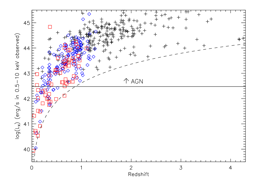
Figure 9.— The observed 0.5-10 keV X-ray luminosities for $z_{\rm conf}\geq 3$ objects with redshift. We label objects classified as “bl” (Type 1 AGN) with black crosses, “nl” with blue diamonds, and “a” with red squares. The dashed line shows the survey’s limiting luminosity from the XMM flux limit. The AGN luminosity cut of $L_{0.5-10\rm keV}=3\times 10^{42}$ is drawn as a solid line: all “nl” and “a” above this line are AGN. Objects below this line, however, are not necessarily inactive: two Type 1 AGN are less luminous, and the luminosity limit is conservative.

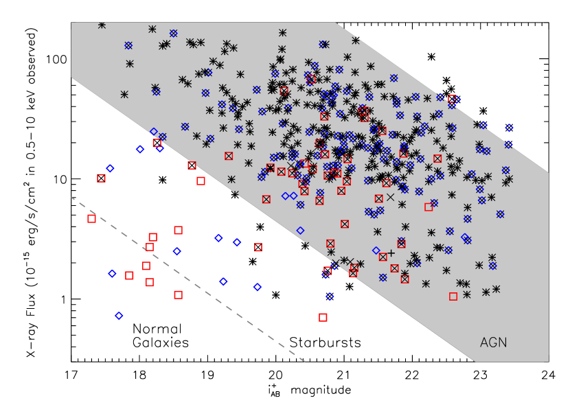
Figure 10.— The X-ray flux vs. the $i_{\rm AB}^{+}$ magnitude for the $z_{\rm conf}\geq 3$ objects. The AGN locus of $-1\leq\log{f_{X}/f_{O}}\leq 1$ (Maccacaro et al., 1988, , see also Equation 2) is shown by the gray shaded region, along with approximate boundary between quiescent and star-forming galaxies at $\log{f_{X}/f_{O}}=-2$ (Bauer et al., 2004). Black crosses are targets classified “bl” (Type 1 AGN), blue diamonds are “nl,” and red squares are “a” objects. We additionally mark all targets of $L_{0.5-10\rm keV}>3\times 10^{42}$ with black x’s. We consider targets either in the AGN locus or with $L_{X}>3\times 10^{42}$ to be AGN: this includes all of the “bl” spectra and all but 53 of the “nl” and “a” spectra.

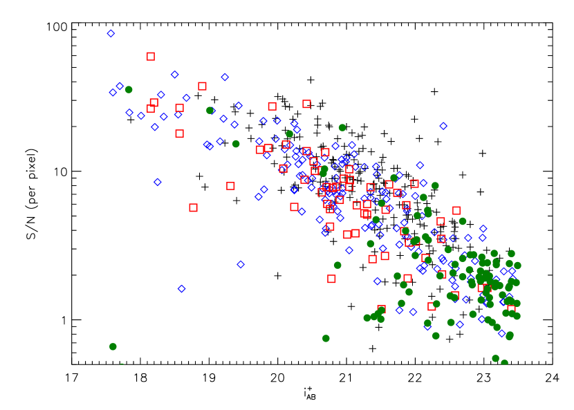
Figure 11.— The signal-to-noise (S/N) and optical $i_{\rm AB}^{+}$ magnitudes for the X-ray targets. Crosses indicate broad emission line spectra, diamonds are narrow emission line spectra, squares are absorption line spectra, and filled circles are unclassified objects. The S/N and optical magnitude are correlated, with scatter from varying conditions over three years of observing. The number of unidentified objects increases greatly at $i_{\rm AB}^{+}>22$, although we still identify emission line spectra at the faintest magnitudes.

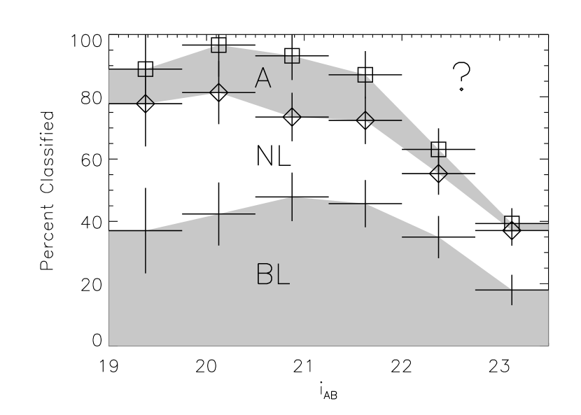
Figure 12.— Cumulative completeness by classification type versus optical $i_{\rm AB}^{+}$ magnitude. Each region (shaded or unshaded) indicates the relative fraction of broad emission line objects (“bl”), narrow emission line objects (“nl”), and absorption line (“a”) spectra. Targets with too low S/N to venture a classification are represented in the upper “?” region. Error bars on the points above each region are calculated assuming that, in each magnitude bin, both the number of each class and the total number have associated Poisson counting errors. The total completeness for each classification is $\sim$90% to $i_{\rm AB}^{+}\leq 22$, although we can correct for the incompleteness of each spectral type to $i_{\rm AB}^{+}\leq 23$.

Figure 13.— Our estimated completeness to assigning $z_{\rm conf}\geq 3$ redshifts for broad emission line spectra (Type 1 AGN). We used Monte Carlo simulations with 20 different spectra with Gaussian-distributed noise for each of 4 values of S/N and 20 redshift bins. Each point represents the number of simulated spectra assigned $z_{\rm conf}\geq 3$, with an additional 36% of the bad $z_{\rm conf}<3$ simulated spectra based on the partial MMT/Hectospec coverage (since 104/288 observed Type 1 AGN had supplemental Hectospec spectra). Each signal-to-noise is associated with an $i_{\rm AB}^{+}$ magnitude according to the median values in Figure 11. The redshift ranges of lowest completeness correspond to observed wavelength ranges with only one emission line, as detailed in §4.3. Almost all of the simulated spectra to which we are not complete are identified as “bl” objects but with degenerate spectra.

Figure 14.— The redshift distributions of broad line (“bl”) AGN, narrow emission line (“nl”) spectra, and absorption line (“a”) galaxies. The raw distributions are shown with squares, while the distributions adjusted for the incompleteness (see §4.3 & 4.4 and Figure 15) are shown with diamonds. We do not correct the “nl” and “a” types where there is no spectroscopic data at $z>1.4$.

Figure 15.— The photometric redshifts for the spectra without high-confidence redshifts. Square symbols show all 192 objects, and diamonds show the 146 $i_{\rm AB}^{+}<23$ objects. The spectral type for these objects comes from the template used for the photometric redshift, with “a” and “nl” fractions estimated as described in §4.4. We use the photometric redshifts and classifications to characterize the complete $i_{\rm AB}^{+}<23$ X-ray AGN sample.

Figure 16.— The absolute magnitude of the AGN (meeting the X-ray criteria of $-1\leq\log{f_{X}/f_{O}}\leq 1$ or $L_{0.5-10\rm keV}>3\times 10^{42}$ ) with redshift. The solid line indicates an arbitrary quasar/Seyfert boundary at $M_{i}=-23$, and the dashed lines indicate fluxes of $i_{\rm AB}^{+}=22$ and $i_{\rm AB}^{+}=23$. Symbols for object types are as in Figures 11 and 12, with crosses for “bl” or “bnl” objects (Type 1 AGN), diamonds for “nl” and “nla” objects (Type 2 AGN), and squares for “a” objects (optically obscured AGN).

Figure 17.— The ratio of obscured to unobscured AGN with redshift. We define obscured AGN as spectra with narrow emission or absorption lines (“nl,” “a,”, and “nla”) that meet the X-ray AGN criteria of §3.2, while unobscured AGN are all broad-line (“bl” and “bnl”) spectra. In the top panel the raw fractions are shown in gray, while the corrected fractions based on the incompleteness (characterized in §4.3 & 4.4) are shown by the black diamonds. The bottom panel shows the ratios for AGN fainter and brighter than the median luminosity $L_{\rm med}=1.32\times 10^{44}$ cgs, with the $L_{0.5-10~{}\rm keV}<L_{\rm med}$ ratio as squares, and the $L_{0.5-10~{}\rm keV}>L_{\rm med}$ ratio as triangles. The errors associated with each point assume that the numbers of objects observed in each redshift bin are Poissonian. Logistic regression analysis shows that the ratio of obscured to unobscured increases with redshift and decreases with luminosity, as shown by the best-fit power-laws.

References

- Abraham et al. (2004) Abraham, R. G. et al. 2004, AJ, 127, 2455
- Adelman-McCarthy et al. (2008) Adelman-McCarthy, J.K. et al. 2008, ApJS, 175, 297-313
- Akylas et al. (2006) Akylas, A., Georgantopoulos, I., Georgakakis, A., Kitsionas, S., & Hatziminaoglou, E. 2006, A&A, 459, 693
- Alexander et al. (2001) Alexander, D. M. et al. 2001, AJ, 122, 2156
- Alexander et al. (2003) Alexander, D. M. et al. 2003, ApJ, 126, 539
- Antonucci (1993) Antonucci, R. 1993, ARA&A, 31, 473
- Baldwin, Philips, & Terlevich (1981) Baldwin, J. A., Phillips, M. M., & Terlevich, R. 1981, PASP, 93
- Ballantyne, Everett, & Murray (2006) Ballantyne, D. R., Everett, J. E., & Murray, N. 2006, ApJ, 639, 740
- Ballantyne (2008) Ballantyne, D. R. 2008, ApJ, 685, 787
- Barger et al. (2003) Barger, A. J. et al. 2003, AJ, 126, 632
- Barger et al. (2005) Barger, A. J., Cowie, L. L., Mushotzky, R. F., Yang, Y., Wang, W.-H., Steffen, A. T., Capak, P. et al. 2005, AJ, 129, 578
- Bauer et al. (2004) Bauer, F. E. , Alexander, D. M., Brandt, W. N., Schneider, D. P., Treister, E., Hornschemeier, A. E., Garmire, G. P., & 2004, AJ, 128, 2048
- Bigelow et al. (1998) Bigelow, B. C., Dressler, A. M., Shectman, S. A., & Epps, H. W. 1998, in Proc. SPIE Vol. 3355, 225, Optical Astronomical Instrumentation, Sandro D’Odorico; Ed.
- Brand et al. (2006) Brand, K. et al. 2006, ApJ, 641, 140
- Brandt, Laor, & Wills (2000) Brandt, W. N., Laor, A., & Wills, B. J. 2000, ApJ, 528, 637
- Brandt & Hasinger (2005) Brandt, W. N. & Hasinger, G. 2005, ARA&A, 43, 827
- Brusa et al. (2008) Brusa, M. et al. 2008, ApJ, in preparation
- Bruzual & Charlot (2003) Bruzual, G. & Charlot, S. 2003, MNRAS, 344, 1000
- Bundy et al. (2007) Bundy, K. et al. 2007, ApJ, 681, 931
- Capak et al. (2007) Capak, P. et al. 2007, ApJS, 172, 99
- Cappelluti et al. (2007) Cappelluti, N. et al. 2007, ApJS, 172, 341
- Cappelluti et al. (2008) Cappelluti, N. et al. 2008, A&A submitted
- Civano et al. (2007) Civano, F. et al. 2007, A&A, 476, 1223
- Civano et al. (2008) Civano, F. et al. 2008, in preparation
- Cocchia et al. (2007) Cocchia, F. et al. 2007, A&A, 466, 31
- Colbert et al. (2004) Colbert, E. J. M., Heckman, T. M., Ptak, A. F., Strickland, D. K., & Weaver, K. A. 2004, ApJ, 602, 231
- Comastri et al. (2002) Comastri, A. et al. 2002, ApJ, 571, 771
- 2dF, Croom et al. (2001) Croom, S. M., Smith, R. J., Boyle, B. J., Shanks, T., Loaring, N. S., Miller, L., & Lewis, I. J. 2001, MNRAS, 322, 29
- Daddi et al. (2007) Daddi, E. et al. 2007, ApJ, 670, 173
- Davis et al. (2007) Davis, M. et al. 2007, ApJ, 660, 1
- Eckart et al. (2006) Eckart, M. E., Stern, D., Helfand, D. J., Harrison, F. A., Mao, P. H., & Yost, S. A. 2006, ApJ, 165, 19
- Eisenstein et al. (2001) Eisenstein, D. J. et al. 2001, AJ, 122, 2267
- Elvis et al. (2008) Elvis, M. et al. 2008, in preparation
- Fabbiano (1989) Fabbiano, G. 1989, ARA&A, 27, 87
- Fabricant et al. (2005) Fabricant, D. et al. 2005, PASP, 117, 1411
- Finoguenov et al. (2008) Finoguenov, A. et al. 2008, in preparation
- Fiore et al. (2003) Fiore, F. et al. 2003, A&A, 409, 79
- Fiore et al. (2008) Fiore, F. et al. 2008, ApJ submitted (astro-ph/0810.0720)
- Fox (1997) Fox, J. 1997, Applied Regression Analysis, Linear Models, and Related Methods (Thousand Oaks, CA: Sage Publications), 438
- Gallagher et al. (2006) Gallagher, S. C., Brandt, W. N., Chartas, G., Priddey, R., Garmire, G. P., & Sambruna, R. M. 2006, ApJ, 644, 709
- Gavignaud et al. (2006) Gavignaud, I. et al. 2006, A&A, 457, 79
- Gilli et al. (2001) Gilli, R., Salvati, M., & Hasinger, G. 2001, A&A, 366, 407
- Gilli et al. (2007) Gilli, R., Comastri, A., & Hasinger, G. 2007, A&A, 463, 79
- Glazebrook & Bland-Hawthorn (2001) Glazebrook, K. & Bland-Hawthorn, J. 2001, PASP, 113, 197
- Green et al. (2004) Green, P. J. et al. 2004, ApJS, 150, 43
- Hasinger et al. (2005) Hasinger, G., Miyaji, T., & Schmidt, M. 2005, A&A, 441, 417
- Hasinger et al. (2007) Hasinger, G. et al. 2007, ApJS, 172, 29
- Hasinger (2008) Hasinger, G. 2008, A&A, 490, 905
- LBQS, Hewett, Foltz, & Chaffee (1995) Hewett, P. C., Foltz, C. B., & Chaffee, F. H. 1995, AJ, 109, 1498
- Hopkins, Richards, & Hernquist (2007) Hopkins, P. F., Richards, G. T., Hernquist, L. 2007, ApJ, 654, 731
- Hornschemeier et al. (2001) Hornschemeier, A. F. et al. 2001, ApJ, 554, 742
- Kauffmann et al. (2003) Kauffmann, G. et al. 2003, MNRAS, 346,1055
- Kelly et al. (2008) Kelly, B. C., Bechtold, J., Trump, J. R., Vestergaard, M., & Siemiginowska, A. 2008, ApJS, 176, 355
- Kewley et al. (2001) Kewley, L. J., Dopita, M. A., Sutherland, R. S., Heisler, C. A., & Trevena, J. 2001, ApJ, 556, 121
- Kim et al. (2004) Kim, D.-W. et al. 2004, ApJ, 600, 59
- Kollmeier et al. (2006) Kollmeier, J. A. et al. 2006, ApJ, 648, 128
- La Franca et al. (2005) La Franca, F. etal 2005, ApJ, 635, 864
- Lawrence & Elvis (1982) Lawrence, A. & Elvis, M. 1982, ApJL, 256, 410
- Lawrence (1991) Lawrence, A. 1991, MNRAS, 252, 586
- Lehmann et al. (2001) Lehmann, I. et al. 2001, A&A, 371, 833
- Lilly et al. (2008) Lilly, S. J. et al. 2008
- Lonsdale et al. (2003) Lonsdale, C. J. et al. 2003, PASP, 115, 897
- Luo et al. (2008) Luo, B. et al. 2008, ApJS, 179, 19
- Maccacaro et al. (1988) Maccacaro, T., Gioia, I. M., Wolter, A., Zamorani, G., & Stocke, J. T. et al. 1988, ApJ, 326, 680
- Maiolino & Rieke (1995) Maiolino, R. & Rieke, G. H. 1995, ApJ, 454, 95
- Martinez-Sansigre et al. (2005) Martinez-Sansigre, A. et al. 2005, Nature, 436, 666
- Moustakas & Kennicutt (2006) Moustakas, J. & Kennicutt, R. C. 2006, ApJ, 651, 155
- Nicastro & Elvis (2000) Nicastro, F. & Elvis, M. 2000, NewAR, 44, 569
- Puccetti et al. (2008) Puccetti et al. 2008, in preparation
- Richards et al. (2006) Richards, G. T. et al. 2006, ApJS, 166, 470
- Rigby et al. (2006) Rigby, J. R., Rieke, G. H., Donley, J. L., Alonso-Herrero, A., & Pérez-González, P. G. 2006, ApJ, 645, 115
- Risaliti & Elvis (2004) Risaliti, G. & Elvis, M. 2004, in Supermassive Black Holes in the Distant Universe, ed. A. J. Barger (Dordrecht, The Netherlands: Kluwer), 187
- Salvato et al. (2008) Salvato, M. et al. 2008, ApJ in press, (astro-ph/0809.2098)
- BQS, Schmidt & Green (1983) Schmidt, M. & Green, R. F. 1983, ApJ, 269, 352
- SDSS, Schneider et al. (2007) Schneider, D. P. et al. 2007, AJ, 134, 102
- Schwope et al. (2000) Schwope, A. D. et al. 2000, AN, 321, 1
- Scoville et al. (2007) Scoville, N. et al. 2007, ApJS, 172, 38
- Silverman et al. (2005) Silverman, J. D. et al. 2005, ApJ, 618, 123
- Simpson (2005) Simpson, C. 2005, MNRAS, 360, 565
- Smolčić et al. (2008a) Smolčić, V. et al. 2008a, ApJS, 177, 14
- Smolčić et al. (2008b) Smolčić, V. et al. 2008b, ApJ in press (astro-ph/0808.0493)
- Spergel et al. (2003) Spergel, D. N., et al. 2003, ApJ, 148, 175
- Steffen et al. (2004) Steffen, A. T., Barger, A. J., Cowie, L. L., Mushotzky, R. F. & Yang, Y. 2004, ApJL, 596, 23
- Sulentic et al. (2000) Sulentic, J. W., Marziani, P., & Dultzin-Hacyan, D. 2000, ARA&A, 38, 521
- Szokoly et al. (2004) Szokoly, G. P. et al. 2004, ApJS, 155, 271
- Treister & Urry (2006) Treister, E. & Urry, C. M. 2006, ApJL, 652, 79
- Treister, Krolik & Dullemond (2008) Treister, E., Krolik, J. H. & Dullemond, C. 2008, ApJ, 679, 140
- Tremonti et al. (2004) Tremonti, C. A. et al. 2004, 613, 898
- Trump et al. (2007) Trump, J. R. et al. 2007, ApJS, 172, 383
- Trump et al. (2008) Trump, J. R. et al. 2008, in preparation
- Ueda et al. (2003) Ueda, Y., Akiyama, M., Ohta, K., & Miyaji, T. 2003, ApJ, 598, 886
- Ueda et al. (2008) Ueda et al. 2008, ApJS, 179, 124
- Urry & Padovani (1995) Urry, C. M. & Padovani, P. 1995, PASP, 107, 803
- Vanden Berk et al. (2001) Vanden Berk, D. E. et al. 2001, AJ, 122, 549
- Vignali et al. (2003) Vignali, C., Brandt, W. N., Schneider, D. P., Garmire, G. P., & Kaspi, S. 2003, AJ, 125, 2876
- Wang et al. (2004) Wang, J. X. et al. 2004, AJ, 127, 213
- HES, Wisotzki et al. (2000) Wisotzki, L., Christlieb, N., Bade, N., Beckmann, V., Köhler, T., Vanelle, C., & Reimers, D. 2000, A&A, 358, 77
- Yang et al. (2004) Yang, Y. et al. 2004, AJ, 128, 1501
- York et al. (2000) York, D. et al. 2000, AJ, 120, 1579
- Zakamska et al. (2003) Zakamska, N. L. et al. 2003, AJ, 126, 2125