The nonequilibrium Ehrenfest gas: a chaotic model with flat obstacles?

Abstract

It is known that the non-equilibrium version of the Lorentz gas (a billiard with dispersing obstacles Sin70 , electric field and Gaussian thermostat) is hyperbolic if the field is small CHE . Differently the hyperbolicity of the non-equilibrium Ehrenfest gas constitutes an open problem, since its obstacles are rhombi and the techniques so far developed rely on the dispersing nature of the obstacles CHE ; Wo1 . We have developed analytical and numerical investigations which support the idea that this model of transport of matter has both chaotic (positive Lyapunov exponent) and non-chaotic steady states with a quite peculiar sensitive dependence on the field and on the geometry, not observed before. The associated transport behaviour is correspondingly highly irregular, with features whose understanding is of both theoretical and technological interest.

Keywords: Non-dispersing billiards, Gaussian thermostat, Bifurcations.
AMS: 82C05, 70Fxx, 82C70

I Introduction

The Ehrenfest model of diffusion (named after the Austrian Dutch physicists Paul and Tatiana Ehrenfest) was proposed in the early 1900s in order to illuminate the statistical interpretation of the second law of thermodynamics and to study the applicability of the Boltzmann equation. In the Ehrenfest wind-tree model EHE , the point-like (”wind”) particles move on a plane and collide with randomly placed fixed square scatterers (”tree”).
This model has been recently reconsidered in DETT to prove that microscopic chaos is not necessary for Brownian motion. A one-dimensional version of this model has been considered in CECC to investigate the origin of diffusion in non chaotic systems. In CECC the authors identify two sufficient ingredients for diffusive behavior in one-dimensional, non-chaotic systems: a) a finite-size, algebraic instability mechanism, and b) a mechanism that suppresses periodic orbits. A nonequilibrium modification of the model, with regularly placed scatterers, has been proposed in LRB to test the applicability of the so called fluctuation relation (ECM2 ; ES ; GC1 ; GC2 ) to non chaotic systems. This modified model was chosen under the assumption that, at small and vanishing fields at least, it must be non-chaotic, since collisions with flat boundaries do not lead to exponential separation of nearby phase space trajectories.
However the question of whether such a model can have positive Lyapunov exponents, as functions of the field, is open. Indeed, the techniques so far developed, e.g. by Chernov and Wojtkowski CHE ; Wo1 , rely on the dispersing nature of the billiard obstacles.
In this paper, the dynamical properties of the nonequilibrium version of the Ehrenfest gas are considered as functions of the field and of the parameters which determine the billiard table. Numerical tests are performed to find chaotic attractors and to compute the Lyapunov exponents. The construction of a sort of bifurcation diagram of the attractor as a function of the electric field and of the geometry is attempted. The result turns out to be quite peculiar: chaotic regimes with an extremely sensitive dependence on the parameters appear possible, although not easy to establish rigorously. If this model can be taken to approximate the transport of matter in microporous membranes, our results confirm the sensitive dependence of microporous transport on all relevant parameters observed e.g. in Bia ; Je-Ro . Indeed, the current of the nonequilibrium Eherenfest gas is proportional to the sum of the Lyapunov exponents (cf. Eq.(11) below), which varies with the parameters as irregularly as the attractors do.

II The model

The billiard table consists of rhombi of side length $l$ with distances along the $x$ and $y$ directions between the centers of two nearest neighbouring rhombi given by $x_{L}$ and $y_{L}$, respectively. The centers of the rhombi are fixed on a triangular lattice in a plane and have coordinates

$$\left(\begin{array}[]{c}x_{c}\\ y_{c}\\ \end{array}\right)=m_{c}\textbf{l}_{1}+n_{c}\textbf{l}_{2},\qquad m_{c},n_{c}\in\mathbb{Z}$$

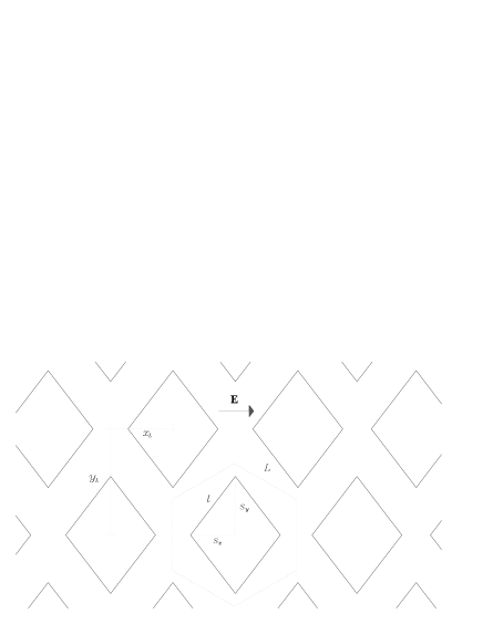
Figure 1: The modified Ehrenfest gas. In the present paper, the side of the elementary cell is set to 1.291, while the semiaxis of the rhombus are chosen to be 1.1 and 0.7573 respectively.

where $\textbf{l}_{1}=(x_{L},0)$ and $\textbf{l}_{2}=(0,y_{L})$ are the lattice vectors. If all the pairs $(m_{c},n_{c})$ are selected, the billiard is invariant under the group of spatial translations generated by $\textbf{l}_{1}$ and $\textbf{l}_{2}$. Accordingly, the whole lattice can be mapped onto a so-called Wigner-Seitz cell, with periodic boundary conditions (Figure 1). The elementary Wigner-Seitz cell of the triangular lattice is a hexagon of length side $L$ and area

$$A_{WS}=|\textbf{l}_{1}\times\textbf{l}_{2}|.$$

The centers of all other cells are identified by the pairs $(m_{c},n_{c})\in\mathbb{Z}^{E}\times\mathbb{Z}^{E}$ or $(m_{c},n_{c})\in\mathbb{Z}^{O}\times\mathbb{Z}^{O}$ where $\mathbb{Z}^{E}=\{n\in\mathbb{Z}:|n|\,\textrm{is even}\},\quad\mathbb{Z}^{O}=\{n\in\mathbb{Z}:|n|\,\textrm{is odd}\}.$ Because of the bi–jective correspondence between rhombi and pairs $(m_{c},n_{c})$, one may label a generic rhombus by $\mathcal{R}_{m_{c},n_{c}}$ and the corresponding hexagon by $\mathcal{H}_{m_{c},n_{c}}$. Further, a label can be put on the sides of the rhombi and of the hexagons, introducing an alphabet $\mathcal{A}=\{r_{1},r_{2},r_{3},r_{4}\}$, starting from the right vertical side and oriented clockwise, for the sides of the rhombi and an alphabet $\mathcal{B}=\{h_{1},h_{2},h_{3},h_{4},h_{5},h_{6}\}$ for the hexagon sides, starting from the right vertical side and oriented clockwise. In this alphabet, the sides of a generic rhombus of the lattice can be labelled by a triple $(\mathcal{R}_{m_{c},n_{c}},s)$ with $s\in\mathcal{A}$, while the hexagon side with a triple $(\mathcal{H}_{m_{c},n_{c}},s)=(m_{c},n_{c},s)$ with $s\in\mathcal{B}$. The rhombi lying in the $y$ axes have $\mathcal{R}_{0,i}=(0,i)$ with $i\in\mathbb{Z}^{O}$ and the ones lying in the $x$ axes have $\mathcal{R}_{j,0}=(j,0)$ with $j\in\mathbb{Z}^{E}$.
The geometry of the model is determined by the side $L$ of the hexagonal Wigner-Seitz cell, so that $x_{L}=\sqrt{3}/{2}$ and $y_{L}=3L/2$. Let $\mathcal{R}_{0}=(0,0)$ be the rhombus with the center in the origin of the Cartesian coordinates, $l$ its sides length, $s_{x}$ and $s_{y}$ the half length of the major and minor diagonals respectively, so that $l=\sqrt{s_{x}^{2}+s_{y}^{2}}$. To prevent the overlap of rhombi, the side length of the rhombus inside one hexagon has to verify

$$0\leq l\leq\dfrac{\sqrt{7}}{2}\,L$$

which implies $0\leq s_{x}\leq x_{L}$. The case with $l=\dfrac{\sqrt{7}}{2}\,L$ corresponds to a billiard table which was recently considered in Bia ; Je-Ro .
Take $l\in\Big{(}0,\dfrac{\sqrt{7}}{2}\,L\Big{)}$, hence $s_{x}<x_{l}$. The horizon of the billiard depends on the quantity $s_{y}$ and in particular on the difference $y_{L}-2s_{y}$. If $s_{y}\geq{y_{L}}/{2}$, the horizon is finite; if $s_{y}<{y_{L}}/{2}$, it is infinite. The infinite horizon case allows collision-free trajectories, parallel to the $x-$axis.
When the dynamics is followed within to the Wigner-Seitz cell, the position of the point particle of mass $M$ must be supplemented by the couple $(m_{c},n_{c})$, in order to determine its actual position in the infinite plane. The space between the rhombi forms the two-dimensional domain, in which the particle moves with velocity $v$ during the free flights, while collisions with the sides of the rhombi obey the law of elastic reflection.
In order to drive the model out of equilibrium, an external electric field parallel to the x-axis, $\textbf{E}=\epsilon\mathbf{\widehat{x}}$ is applied. If there were no interaction with a thermal reservoir, any moving particle would be accelerated by the external field, on average, leading to an indefinite increase of energy in the system, and there would be no stationary state. Therefore, in LRB the particle has been coupled to a Gaussian thermostat. The resulting model, with periodically distributed scatterers, has been called the non-equilibrium Ehrenfest gas. Its phase space has four coordinates $(x,y,p_{x},p_{y})$ and its equations of motion are given by

$$\left\{\begin{array}[]{ll}\dot{x}={p_{x}}/{M}~{},\qquad\dot{p_{x}}=\epsilon-\alpha(\textbf{p})p_{x}\\ \dot{y}={p_{y}}/{M}~{},\qquad\dot{p_{y}}=-\alpha(\textbf{p})p_{y}\end{array}\qquad\mbox{with }~{}~{}~{}~{}\alpha(\textbf{p})=-\epsilon p_{x}\right.$$ (1)

where $\epsilon$ is the electric field and $\alpha$ the Gaussian thermostat. The quantity $-\textrm{div}(\dot{\textbf{p}},\dot{\textbf{q}})=\alpha=\epsilon p_{x}$ is known as the phase space contraction rate. Because of the Gaussian thermostat, $p_{x}^{2}+p_{y}^{2}$ is a constant of motion, hence there are only three independent variables, and one may replace $p_{x}$ and $p_{y}$ by the angle $\theta\in(-\pi,\pi]$ that $\textbf{p}=p(\cos\theta,\sin\theta)$ forms with the $x$-axis. For sake of simplicity, we set $M=1$ and $p=1$.
Then, if $(x_{t},y_{t})$ denotes the position at time $t$ and $\theta_{t}$ the velocity angle, measured with respect to the $x$-axis, the trajectory between two collisions reads Ro3

$$\left\{\begin{array}[]{ll}x_{t}=x_{0}-\frac{1}{\epsilon}\ln\frac{\sin\theta_{t}}{\sin\theta_{t_{0}}}\\ y_{t}=y_{0}-\frac{1}{\epsilon}(\theta_{t}-\theta_{t_{0}})\\ \tan\frac{\theta_{t}}{2}=\exp(-\epsilon(t-t_{0}))\tan\frac{\theta_{t_{0}}}{2}\end{array}\right.$$ (2)

where $t_{0}$ is the time of the previous collision, while the collision map $C$ is given by

$$\left\{\begin{array}[]{ll}x^{\prime}_{t}=x_{t}\\ y^{\prime}_{t}=y_{t}\\ \theta^{\prime}_{t}=-\theta_{t}\pm 2\theta\end{array}\right.$$ (3)

where $\theta_{t}$ is the incidence angle, $(x_{t},y_{t})$ is the collision point and $\theta$ is the angle that the side of the rhombus makes with the $x-$axis. The sign $\pm$ depends on the side on which the bounce occurs. Hence $C$ is piecewise linear in $\theta_{t}$.
Considering the dynamics as a geodesic flow on a Riemann manifold, the appropriate metric for this system is Wo-Li ; DET ; MOR

$$ds^{2}=e^{-2\epsilon x}(dx^{2}+dy^{2})$$

which implies that the quantities $\pi_{y}=e^{-\epsilon x}p_{y}$ and $\phi_{t}=\theta_{t}+\epsilon y_{t}=\theta_{t_{0}}+\epsilon\theta$ are conserved. Also, the path length $\mathcal{L}(P_{0},P_{t})$ between $P_{0}=(x_{0},y_{0},\theta_{t_{0}})$ and $P_{t}=(x_{t},y_{t},\theta_{t})$ turns out to be

$$\mathcal{L}(P_{0},P_{t})=\frac{1}{\epsilon}e^{-\epsilon x_{0}}\,\sin\theta_{t_{0}}\,|\cot\theta_{t_{0}}-\cot\theta_{t}|.$$ (4)

III Periodic orbits and stability matrices

Using the symbols introduced above, a trajectory segment $\Omega_{N}$ which consists of $N$ collisions can be labelled by a finite symbolic sequence such as $(\mathcal{R}_{i_{1},j_{1}},s_{1})(\mathcal{R}_{i_{2},j_{2}},s_{2})\dots(\mathcal{R}_{i_{N},j_{N}},s_{N})$, with $(i_{c},j_{c})\in\mathbb{Z}^{E}\times\mathbb{Z}^{E}$ or $(i_{c},j_{c})\in\mathbb{Z}^{O}\times\mathbb{Z}^{O}$ and $s_{c}\in\mathcal{A}$ for $c=1,\dots,N$. Periodic trajectories will be labelled by sequences which are infinitely many copies of a fundamental finite sequence.
There are two types of periodic orbits; those that are periodic in the plane, i.e. that return to the initial point in the plane (they are closed: $\Delta x_{i}=0$, $\Delta y_{i}=0$) and those whose periodicity relies upon the periodicity of the triangular lattice, and return to the same relative position in a different cell (they are open: $\Delta x_{i}\neq 0$ or $\Delta y_{i}\neq 0$).

The velocity vectors of the closed orbits with two collisions have to be orthogonal to both sides of the rhombi where collisions occur. This implies $\theta_{0}=\frac{\pi}{2}+\theta$ and $\theta^{\prime}_{0}=\frac{\pi}{2}-\theta$, where $\theta_{0}$ is the out-going velocity angle and $\theta^{\prime}_{0}$ the in-coming angle, because the absolute value of the velocity angle decreases and preserves the sign during the free flight Ro3 . Then, the closed period-two orbits fly between rhombuses in the same line parallel to the $y$-axes, and have period $\tau$ and length $\mathcal{L}$ given by CBthesis

$$\tau=\frac{2}{\epsilon}\ln\frac{\tan\Big{(}\frac{\pi}{4}+\frac{\theta}{2}\Big{)}}{\tan\Big{(}\frac{\pi}{4}-\frac{\theta}{2}\Big{)}}~{},\qquad\mathcal{L}=\frac{2}{\epsilon}e^{-\epsilon x_{0}}\sin\theta~{}.$$

Now, fix the geometry of the model through the parameters $L>0$, $s_{x}>0$, $s_{y}>0$ and take the initial conditions

$$\Big{\{}x_{0},\,y_{0}=\pm y_{l},\,\theta_{0}=\pm\dfrac{\pi}{2}\Big{\}}.$$

It is easy to show that the periodic orbits $(\mathcal{R}_{0,0},r_{4})(\mathcal{R}_{0,2},r_{3})$ (Figure 2, left panel) and $(\mathcal{R}_{0,0},r_{3})(\mathcal{R}_{0,-2},r_{4})$, with electric field

$$\epsilon=\dfrac{-\theta+\tan\theta\,\ln\cos\theta}{\mp y_{0}+m\,x_{0}+s_{y}}~{},$$ (5)

exist if and only if CBthesis

$$\dfrac{2\theta}{3L}<\epsilon<\dfrac{2\theta}{3L-2s_{y}}.$$ (6)

For open orbits with two collisions in the finite horizon case, simple algebra shows that the following symbolic representations $(\mathcal{R}_{i,j},r_{4})(\mathcal{R}_{i-1,j+1},r_{2})(\mathcal{R}_{i+2,j},r_{4})$ and $(\mathcal{R}_{i,j},r_{1})(\mathcal{R}_{i+3,j+1},r_{3})(\mathcal{R}_{i+2,j},r_{1})$ cannot be realized. However, orbits with symbolic representation $(\mathcal{R}_{i,j},r_{4})(\mathcal{R}_{i+1,j+1},r_{3})(\mathcal{R}_{i+2,j},r_{4})$, and its symmetric counterpart $(\mathcal{R}_{i,j},r_{3})(\mathcal{R}_{i+1,j-1},r_{4})(\mathcal{R}_{i+2,j},r_{3})$ (Figure 2, right panel) do exist. Their period is given by

$$\tau=\frac{2}{\epsilon}\,\ln\frac{1}{\tan(\frac{\pi}{4}-\theta)}.$$

Figure 2: The closed periodic-two orbit $\Omega^{o}_{2}=(\mathcal{R}_{-1,-1},r_{4})(\mathcal{R}_{1,1},r_{3})$ for $\theta=\frac{\pi}{11}$, $x_{l}=\frac{5\sqrt{3}}{3}$ (left panel). The open periodic orbit $\Omega^{o}_{2}=(\mathcal{R}_{0,0},r_{4})(\mathcal{R}_{1,1},r_{3})(\mathcal{R}_{2,0},r_{4})$ for $x_{l}=2$, $s_{x}=0.8$, $s_{y}=0.5$ (right panel).

The open periodic orbits with four collisions (Figure 5, left panel) and symbolic sequence $(\mathcal{R}_{0,0},r_{4})(\mathcal{R}_{-1,1},r_{2})(\mathcal{R}_{1,1},r_{3})(\mathcal{R}_{0,0},r_{1})(\mathcal{R}_{2,0},r_{4})$, and its simmetric image $(\mathcal{R}_{0,0},r_{3})(\mathcal{R}_{-1,-1},r_{1})(\mathcal{R}_{1,-1},r_{4})(\mathcal{R}_{0,0},r_{2})(\mathcal{R}_{2,0},r_{3})$ do exist if CBthesis

$$\max\Big{\{}-s_{x},-x_{l}+\dfrac{1}{\epsilon}\ln\dfrac{\sin\theta^{\prime}_{0}}{\sin\theta_{0}}\Big{\}}<x_{0}<\min\Big{\{}-x_{l}+s_{x}+\dfrac{1}{\epsilon}\ln\dfrac{\sin\theta^{\prime}_{0}}{\sin\theta_{0}},0\Big{\}}$$ (7)

To compute the Lyapunov exponents for these orbits and any other trajectory, consider the stability matrix $J_{S}$ for a trajectory as the product of free flight stability matrices $J_{F}$ and collision stability matrices $J_{C}$

$$J_{S}=\prod_{i=1}^{n}J_{C}(i)J_{F}(i)$$

The number of degrees freedom for the billiard map is two and the variables that we will use are $(x_{0},\theta_{0})$. Thus

$$J_{C}=\begin{pmatrix}\frac{\partial\theta^{\prime}}{\partial\theta_{0}}&\frac{\partial\theta^{\prime}}{\partial x_{0}}\\ \frac{\partial x^{\prime}_{0}}{\partial\theta_{0}}&\frac{\partial x^{\prime}_{0}}{\partial x_{0}}.\end{pmatrix}=\begin{pmatrix}-1&0\\ 0&1\end{pmatrix}$$

The free flight matrix $J_{F}$ depends on the side which the trajectory leaves and the one which it reaches. There are two different types of side, the ones with positive slope, of equation $y=\tan\theta\,x+c$ and the ones with negative slope, of equation $y=-\tan\theta\,x+d$, where $c$ and $d$ are real numbers.
Let us compute the free flight matrix $J_{+,-}$ of a trajectory which goes from a side with positive slope to a side with negative slope. Let $(x_{0},y_{0},\theta_{0})$ and $(x^{\prime}_{0},y^{\prime}_{0},\theta^{\prime}_{0})$ be the initial condition on a side with positive slope and the final condition on a side with negative slope respectively. By using the equations of the trajectory and by the implicit function theorem CBthesis ; IFT we obtain the Jacobian matrix of the free flight:

$$J_{+,-}=\begin{pmatrix}\dfrac{(\tan\theta_{0}+\tan\theta)\,\tan\theta^{\prime}_{0}}{(\tan\theta^{\prime}_{0}+\tan\theta)\,\tan\theta_{0}}&\dfrac{2\epsilon\,\tan\theta\,\tan\theta^{\prime}_{0}}{\tan\theta^{\prime}_{0}+\tan\theta}\\ &\\ -\dfrac{1}{\epsilon\,\tan\theta_{{}_{0}}}\,\dfrac{\tan\theta_{0}-\tan\theta^{\prime}_{0}}{\tan\theta^{\prime}_{0}+\tan\theta}&\dfrac{\tan\theta^{\prime}_{0}-\tan\theta}{\tan\theta^{\prime}_{0}+\tan\theta}\end{pmatrix}$$ (8)

Similarly, the flights from a side with negative slope to a side with positive slope yield

$$J_{-,+}=\begin{pmatrix}-\dfrac{(\tan\theta_{0}-\tan\theta)\,\tan\theta^{\prime}_{0}}{(-\tan\theta^{\prime}_{0}+\tan\theta)\,\tan\theta_{0}}&\dfrac{2\epsilon\,\tan\theta\,\tan\theta^{\prime}_{0}}{-\tan\theta^{\prime}_{0}+\tan\theta}\\ &\\ -\dfrac{1}{\epsilon\,\tan\theta_{{}_{0}}}\,\dfrac{\tan\theta^{\prime}_{0}-\tan\theta_{0}}{\tan\theta-\tan\theta^{\prime}_{0}}&\dfrac{\tan\theta^{\prime}_{0}+\tan\theta}{\tan\theta^{\prime}_{0}-\tan\theta}\end{pmatrix}~{},$$ (9)

and those from one side to a parallel one yield

$$J_{\pm,\pm}=\begin{pmatrix}\dfrac{(\tan\theta_{0}\mp\tan\theta)\,\tan\theta^{\prime}_{0}}{(\tan\theta^{\prime}_{0}\mp\tan\theta)\,\tan\theta_{0}}&0\\ &\\ -\dfrac{1}{\epsilon\,\tan\theta_{{}_{0}}}\,\dfrac{\tan\theta_{0}-\tan\theta^{\prime}_{0}}{\tan\theta^{\prime}_{0}\mp\tan\theta}&1\end{pmatrix}~{}.$$ (10)

If $\mu_{1}$ and $\mu_{2}$ are the eigenvalues of the stability matrix $J_{S}$ for a periodic orbit of period $\tau$, the two Lyapunov exponents are $\lambda_{i}=\dfrac{1}{\tau}\log|\mu_{i}|$, $i=1,2$, and one obtains

$$j=\frac{\Delta x}{\tau}=-\frac{(\lambda_{1}+\lambda_{2})}{\epsilon}$$ (11)

where $j$ is the current and $\Delta x$ is the corresponding displacement in the direction of the field Ro3 . Both the Lyapunov exponents of the closed periodic orbits, with period two, vanish. Indeed, consider that this periodic orbit has $\Delta x=0$, hence $\lambda_{1}+\lambda_{2}=0$. Furthermore, the stability matrix of these periodic orbits, which is $J_{S}=J_{C}J_{-,+}J_{C}J_{+,-}$, is given by

$$J_{S}=\begin{pmatrix}\dfrac{4\tan^{2}\theta-(1-\tan^{2}\theta)}{(1+\tan^{2}\theta)^{2}}&\dfrac{4\epsilon\tan\theta(\tan^{2}\theta-1)}{(1+\tan^{2}\theta)^{2}}\\ &\\ \dfrac{4\epsilon\tan\theta(\tan^{2}\theta-1)}{(1+\tan^{2}\theta)^{2}}&-\dfrac{4\tan^{2}\theta-(1-\tan^{2}\theta)}{(1+\tan^{2}\theta)^{2}}\end{pmatrix}$$

whose determinant is 1, while its trace vanishes. This, implies that both Lyapunov exponents vanish.

IV Numerical estimates of Lyapunov exponents

In this paper, a system is called chaotic when it has at least one positive Lyapunov exponent. We note that the boundary of our system is not defocussing and the external field has a focussing effect, so the overall dynamics should not be chaotic in general, although it is not obviuos that this is the case for all values of the electric field $\epsilon$. In this section we examine the stationary state and the Lyapunov exponents, obtained by using the algorithm developed by Benettin, Galgani, Giorgilli and Strelcyn BGGS , for different values of $\epsilon$, ranging from small to large fields.

IV.1 Chaos for large electric fields

Numerical simulations of the model starting with random initial conditions and electric field in the range $[0.02,1]$ have been initially performed for a trajectory of length $n=10^{7}$ collisions. The parameters chosen for the geometry are $L=1.291$, $s_{x}=0.7573$ and $s_{y}=1.1$ which correspond to a case in which the angles of the rhombi are irrational w.r.t. $\pi$, then, according to a conjecture by Gutkin GU , the equilibrium version of this model, (i.e. the $\epsilon=0$ case), should be ergodic. For simulations of $10^{7}$ collisions, Figure 3 shows that the fields which appear to lead to one positive Lyapunov exponent cover a range larger than that which appears to correspond to two negative exponents. However, do $10^{7}$ collisions suffice for a generic trajectory to characterize the stationary state? For the cases with two negative exponents the answer is affirmative, since the trajectory is clearly captured by an attracting periodic orbit. But the cases with one apparently positive exponent are not equally clear. As LRB already noted, the doubt is that, starting from a generic initial condition, convergence to the steady state might be too slow to be discovered, for reasons which had not been investigated. Indeed, even in cases in which convergence is observed, the particle often appears to peregrinate in a sort of chaotic quasi steady state for very long times, before eventually settling on a periodic or quasi-periodic steady state. Ref. LRB suggested this might always be the case.

Therefore, we extended the simulations of the cases with one apparently positive Lyapunov exponent, up to $1.5\times 10^{8}$ collisions. The behaviour of the system still appears to be non trivial, in cases such as that of $\epsilon=0.374$. Furthermore, plotting the last $10^{4}$ iterates of a trajectory of length $5\times 10^{7}$ collisions, we cover a large fraction of the phase space, which appears quite close to that covered by the last $10^{4}$ iterates of a trajectory of $1.5\times 10^{8}$ collisions (Figure 4).
The conclusion that a chaotic stationary state has been reached seems reasonable in this case, as the computed positive Lyapunov exponent also indicates, having apparently converged to $0.144$ with three digits of accuracy, after only $10^{6}$ collisions.
To strengthen this results, we have looked for an unstable periodic orbit embedded in the attractor, and we have found one periodic orbit of period four, which apparently lies in the attractor and has a positive Lyapunov exponent (Figure 5, right panel). The other possibility is that the orbit is isolated, and is separated from the attractor by such a small neighborhood that is numerically impossible to resolve.
Another interesting example is given by $\epsilon=0.5$: the last $7000$ points of a trajectory of length $5\times 10^{7}$ collisions are compared with the last $10^{4}$ points of the trajectory of length $2\times 10^{8}$ (Figure 6). Also in this case the stationary state seems to have been reached, and a periodic orbit of period four with one positive Lyapunov exponent seems to be embedded in the attractor, similarly to the case of $\epsilon=0.374$. The values of $\epsilon$, of the initial conditions and the Lyapunov exponents are reported in table I and II.

Figure 3: The largest Lyapunov exponent $\lambda_{1}$ for electric fields between $0.02$ and $1$, for trajectories with $10^{7}$ collisions, and random initial condition.

Figure 4: The last $10^{4}$ iterates of the bounce map for $\epsilon=0.374$ out of a trajectory of $5\times 10^{7}$ collisions (left panel) and for a trajectory of $1.5\times 10^{8}$ collisions, starting from the last phase space point of the previous trajectory (right panel). The distribution appears to be the same, suggesting that the system is in an apparently stationary state. Here, $\eta=\cos\varphi$, with $\varphi$ the angle between the outgoing velocity and the side of the rhombus, and $r$ is the perimetral distance of the collision point from the right corner of the rhombus ($\eta$ and $r$ are called Birkhoff coordinates).

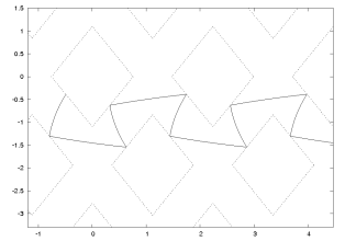
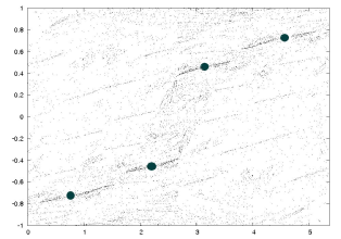
Figure 5: The open period-four orbit $(\mathcal{R}_{0,0},r_{3})(\mathcal{R}_{-1,-1},r_{1})(\mathcal{R}_{1,-1},r_{4})(\mathcal{R}_{0,0},r_{2})(\mathcal{R}_{2,0},r_{3})$ in the plane for $\epsilon=0.374$, $s_{y}=0.7573$, $s_{x}=1.1$, $L=1.291$, $\theta_{0}=-2.0619$, $x_{0}=-0.4885$ (left panel). The four points of this periodic orbit, are inflated to show their embedding in the attractor (right panel). The coordinates are as in Figure 4.

Figure 6: The last 7000 points of the bounce map for $\epsilon=0.5$ out of a trajectory of length $5\times 10^{7}$ collisions (left panel) and the last $10^{4}$ points of a trajectory of length $2\times 10^{8}$ with same $\epsilon$ (right panel). The coordinates are defined as in Figure 4.

Field	Collisions	Lyapunov exponent
0.374	$10^{6}$	0.144232
0.374	$1.5\times 10^{7}$	0.144317
0.374	$6.5\times 10^{7}$	0.144291
0.374	$2.15\times 10^{8}$	0.144320
0.5	$5\times 10^{7}$	0.166648
0.5	$2\times 10^{8}$	0.166622

Table 1: Numerically computed Lyapunov exponents for different trajectories and fields.

Field	$x_{0}$	$y_{0}$	$\theta_{0}$	$\lambda_{1}$	$\lambda_{2}$
0.374	$-0.48971578282741385$	$-0.3886737605834475$	$-2.06199461833$	$0.108316$	$-0.281452$
0.5	$0.30576674801010$	$0.6558650167554337$	$-0.31873995693500$	$0.155569$	$-0.384674$

Table 2: Initial conditions and Lyapunov exponents of periodic orbits of period four. All data have been computed analitically.

IV.2 Chaos for small electric fields

Numerical simulations of the model were performed starting with random initial conditions and considering the electric field in the interval $[0.002,0.1]$, for trajectories of length $n=10^{7}$. Looking at Figure 7 (left panel) we find more cases with one apparently positive Lyapunov exponent than with two negative exponents. Plotting the last $10^{4}$ points, in trajectories of length $1.5\times 10^{8}$, for the electric fields that produced apparently positive Lyapunov exponents, the situation is pratically the same as for large fields: some cases with one exponent that appeared to be positive after $10^{7}$ collisions eventually produce (after $1.5\times 10^{8}$ collisions) two negative exponents and a periodic or quasi-periodic steady state LRB . We have further increased the number of collisions up to $3\times 10^{8}$, but the exponent $\lambda_{1}$ remained positive in most of the cases (Figure 7, right panel) and an apparently chaotic attractor was reached.

Figure 7: The largest Lyapunov exponent, $\lambda_{1}$, for different lengths of trajectory: $10^{7}$ (left panel) and $3\times 10^{8}$ (right panel) for $\epsilon\in[0.002,0.1]$ and random initial condition.

IV.3 A small basin of attraction

The behaviour illustrated above is rather peculiar and calls for some explanation. How can it be that a steady state is so hard to reach in so many cases? Usually, convergence to an attracting periodic orbit occurs rather quickly, while doubts remain in some of the cases we considered even after $10^{8}$ iterations of the bounce map. Therefore, we have investigated in greater detail the specific example with $\epsilon=0.087$, $L=1.291$, $s_{x}=0.7573$ and $s_{y}=1.1$. One finds that the largest time dependent Lyapunov exponent, $\lambda_{1}$, rapidly settles on a positive value, as if the trajectory had reached a chaotic attractor. However, for randomly chosen initial conditions, a striking and precise monotonic $1/n$ behavior sets in for $\lambda_{1}$, after a critical, typically large, time $N_{c}$ (cf. left panel of Figure 8), as if the trajectory had eventually collapsed on an attracting periodic orbit. Indeed, the asymptotic value of $\lambda_{1}$ is $-0.004838$ with an estimated error not larger than $10^{-6}$ . The accuracy of this result is due to the fact that a sufficiently long simulation approaches an attracting periodic orbit to practically full numerical precision; the Lyapunov exponents can then be computed with analogous accuracy. This is particularly true in the present example, which turns out to have an attracting orbit made of only 19 points, whose initial condition, up to 12 digits accuracy, is given by $x_{\rm po}=0.418447478686,y_{\rm po}=0.492193019206,\theta_{\rm po}=0.718794450586$, (cf. right panel of Figure 8). For such a small number of points, numerical errors cannot appreciably affect the result. In particular, no doubts remain, in this case, about the negative sign of both exponents, hence about the attracting nature of the orbit.

The question now arises as to the shape and size of the basin of attraction $\mathcal{B}$ of the asymptotic periodic orbit, because a particle with random initial conditions wonders around almost all phase space before falling inside this set.

Our analysis of the evolution of trajectories, with initial condition close to the attracting periodic orbit, shows that $\mathcal{B}$ is quite limited in size, and particularly hard to reach because it contains a very small region around the right vertex of the rhombus. Furthermore, by varying the initial conditions around $(x_{\rm po},y_{\rm po},\theta_{\rm po})$, and computing the Lyapunov exponents, the irregular shape of $\mathcal{B}$ is evidenced by the times $N_{c}$, which vary most irregularly from $O(10)$ to $O(10^{8})$, $O(10^{8})$ being typical for random initial conditions. Nevertheless, the radius of $\mathcal{B}$, i.e. the supremum distance between any two points of $\mathcal{B}$, is not smaller than $10^{-4}$, which is quite small but well above the distances which can be accurtely measured with double precision numerical simulations.

We conclude that $\mathcal{B}$ lies at the border of a chaotic repeller TCTel , and that it is quite small and of irregular shape. Hence, only after a sufficiently long peregrination in phase space, when the transiently chaotic trajectory gets sufficiently close to $\mathcal{B}$, may numerical errors let the trajectory jump inside $\mathcal{B}$. At this stage, the sudden (exponential) convergence of the trajectory and the consequent $1/n$ behaviour of the Lyapunov exponents begin.

The same qualitative behaviour has been observed for $\epsilon=$0.002, 0.003, 0.004, 0.005, 0.006, 0.007, 0.010, 0.022, 0.040, 0.041, 0.042, 0.043, 0.050, 0.064, 0.065, 0.073, 0.087.

Figure 8: Behaviour of the finite time Lyapunov exponents $\lambda_{1,2}$ with the number of collisions $n$, for $\epsilon=0.087$ (left panel). The logarithmic scale in $n$ clearly separates the initial, intermediate and asymptotic regimes. The exponents rapidly converge to one positive and one negative value, which persist for very long, up to a number $N_{c}$ of collisions, dependent on the initial condition. After $N_{c}$, both exponents converge as $1/n$ to the value $-0.004838$. For random initial conditions, $N_{c}$ is of order $O(10^{8})$, for initial conditions close to the asymptotic periodic orbit (right panel), $N_{c}$ varies irregularly between $O(10)$ and $O(10^{7})$. The right panel reports the last $10^{4}$ points of $3\cdot 10^{8}$ collisions, which testifies that the motion has settled on a periodic orbit of 19 points only. The coordinates are defined as in Figure 4.

V Behaviour of the attractor

It is interesting to understand the behaviuor of the steady state with the field, i.e. to build a kind of bifurcation diagram, e.g. to compare with the one for the Lorentz gas, whose obstacles are defocussing Ro3 . Our analysis reveals substantial differences from the case of Ro3 , as well as from standard low dimensional dynamics.

V.1 Multi-furcation as function of the electric field

In order to visualize the behaviour of the attractor as a function of the electric field, we consider a projection of the billiard map phase space: the projection onto the $\theta$ axis, which shows a sort of “multi-furcation” scenario. When the field is varied, a series of dramatic changes in the dynamics occurs.
For the geometry determined by $L=1.291$, $s_{x}=0.7573$ and $s_{y}=1.1$, numerical simulations were performed for a random initial condition, ignoring the initial transient behaviour, for the electric fields in the range $[0.01,1]$ with a step $\Delta\epsilon=0.01$. At the end of a trajectory of $10^{7}$ collisions, the last $10^{3}$ points were plotted (Figure 9, presents only the upper half projection onto the $\theta$ axis; the other half of this diagram is trivially obtained from this, by reflection along the line $\theta=0$, as a result of the symmetry imposed on the system by the external field). In this way, many electric fields are found whose dynamics sample most of the $\theta$ space, while only a few fields show a periodic (or quasi periodic) steady state. The apparently chaotic regions and the regular regions are finely interspersed with each other, in a way which we have not found elsewhere in the literature.
We have performed simulations also in the range $[1,1.3]$ and have only plotted the last $10^{3}$ points out of $10^{7}$ collisions, as in the previous case. In this range, all attractors have been found to be periodic orbits, which are reached well before $10^{7}$ collisions. In other words, the stationary state is rapidly reached with large electric fields as expected for the correspondingly high dissipations.
How conclusive are these results? Again, when a periodic steady state is reached, the situation is clear, while doubts remain when the steady state looks chaotic. Therefore we have considered the range $[0.77,0.86]$: a rather wide range, apparently chaotic, but also characterized by high dissipation, which favours ordered dynamics. Running trajectories of $10^{8}$ collisions and plotting the last $10^{3}$ points, the apparently weakly chaotic states survived, despite the high dissipation. This study combined with the analysis of the largest Lyapunov exponent makes chaos quite plausible for these fields, although we cannot exclude that the trajectories collapse on periodic orbits after much longer times. On the other hand, there is no purpose in pushing further this analysis, since it is bound to remain uncertain. Here, it suffices to have uncovered a rather peculiar behaviour, unexpected for simple dynamical systems.
Indeed, in our model, the passage from low-period attractors to apparently chaotic steady states, is rather abrupt and seems to be discontinuous. Moreover, the periodic attractors always seem to coexist with transiently chaotic states. Differently, standard bifurcation scenarios are characterized by a gradual growth of the period of the attracting orbits, the orbits are globally attracting and lead to fast convergence of the trajectories towards them. To further investigate this behaviour, we have honed the range $[0.77,0.78]$ with step $0.001$ simulating trajectories of $10^{8}$ collisions, finding a (quasi) periodic orbit at $\epsilon=0.771$ and another one at $\epsilon=0.777$, with apparently chaotic trajectories in the middle. Thus, we have further honed the range $[0.770;0.771]$ with a step of $0.0001$, to find that a jump from (quasi) periodic orbits to apparent chaos happens for a field variation of just $10^{-5}$.
We have also performed simulations in the range $[0.771,0.772]$, namely from the (quasi) periodic orbit at $\epsilon=0.771$ to an apparently chaotic case at $\epsilon=0.772$. Plotting the last $10^{3}$ points of trajectories of $10^{8}$ collisions, apparent chaos and (quasi) periodic orbits appear again to be finely intertwined. The range $[0.18,0.38]$ was similarly studied, and some of the cases that appeared to be chaotic after $10^{7}$ collisions, turned into (quasi) periodic after $10^{8}$, but not all. Therefore, the duration of the transients results exceedingly long in all cases, which is a manifestation of either very small basins of attraction, or of the smallness of the stable islands, whose size would then vary wildly with the field. Although this is not conclusive evidence, our analysis supports the idea that there could be a discontinuous transition between chaos and regular motion, in the non-equilibrium Ehrenfest gas.

Figure 9: The upper half of the projection of the multi-furcation diagram onto the $\theta$ axis, for $\epsilon$ in the range $[0.01;1]$. The last $10^{3}$ points of trajectories with length $10^{7}$ collisions have been plotted (left panel). The multi-furcation diagram in the $(\epsilon;\theta)$ plane, for $\epsilon$ in the range $[1,1.3]$, from the last $10^{3}$ collisions out of a trajectory of $10^{7}$ collisions (right panel).

V.2 Dependence on the geometry

In this section we outline the behaviour of the attractors as functions of one of the parameters which determine the shape of the billiard: $s_{x}$. We take two electric fields (one large and one small) for which we had found apparently chaotic behaviours.
Let $\epsilon=0.374$ be the electric field, $L=1.291$ and $s_{y}=1.1$; we study the attractor reliance on $s_{x}\in[0,1]$ with step $0.01$. We considered trajectories of length $10^{7}$ collisions and looked at the last $10^{3}$ points. We found a complicated scenario, analogous to the one for the dependence on $\epsilon$, as $s_{x}$ was varied. In the chosen range, there are more cases with apparently chaotic attractors than with (quasi) periodic steady states. Increasing the number of collisions in each trajectory up to $5\times 10^{7}$, we find that apparent chaos persists, in other words it seems that the effect of the electric field prevails on the geometry effects. To analyze more carefully this fact, we have honed the interval $[0.09,0.1]$ for $s_{x}$, with step $0.0005$ and for trajectories of $10^{8}$ collisions. A sudden transition between apparent chaos and periodic orbits happens at $s_{x}=0.099$.
For $\epsilon=0.014$, $s_{x}$ was taken in $[0,1]$ with step $0.01$, for trajectories of length $10^{7}$ collisions. We found that the situation is slightly different from the small field case. The apparently chaotic steady states occupy a smaller region of the phase space than the steady states of the $\epsilon=0.374$ case. For instance, the asymptotic state of $\epsilon=0.014$ seems to fill almost completely the space $\theta$, differently from the case of $\epsilon=0.374$. Increasing the length of the trajectories up to $5\times 10^{7}$ collisions, various apparently chaotic cases reduce to (quasi) periodic orbits, while other survive. Finally, we increased the number of collisions up to $10^{8}$ for $\epsilon=0.014$ again finding that some apparently chaotic cases turned into quasi periodic cases, while other survived.
We conclude that the dependence of the attractors on the parameter $s_{x}$ is qualitatively similar to the dependence on $\epsilon$, although at times the dependence on $\epsilon$ prevails.

VI Conclusion

In this paper we have examined the non equilibrium version of the Ehrenfest gas, which is a billiard model with an electric field and a Gaussian thermostat, whose point particle moves in the plane and undergoes elastic collisions with rhomboidal obstacles. The motivation was to understand the dynamics of this nonequilibrium model, whose obstacles have flat surfaces, hence do not defocus the trajectories, while its thermostat, which makes dissipative the dynamics, does focus them . We have shown that periodic orbits with one positive Lyapunov exponent embedded in what appear to be chaotic attractors, do exist. Our numerical results have identified electric fields whose dynamics is strongly suggested to be chaotic, although conclusive results are out of reach at present, because of a very peculiar phenomena. The stationary state, even if attracting and trivial, requires very long times to be reached, because it coexists with a transiently chaotic state which covers most of the phase space. The dependence on the model parameters of the steady state behaviour also presents peculiar features which, to the best of our knowledge, have not been observed before: a very irregular, possibly discontinuous dependence of the attracting orbit, and/or of the size and shape of the stable islands, on $\epsilon$ and $s_{x}$. The peculiarity remains even if it is eventually proved that all steady states are periodic, because of their coexistence with transiently chaotic states, and because of the consequent irregular behaviour of the convergence rates. As the sum of the Lyapunov exponents is proportional to the travelled distance, cf. Eq.(11), very irregular transport properties are obtained as well, perhaps as irregular as those conjectured for other low-dimensional dynamical systems kla .

VII Acknowledgements

We would like to thank M. P. Wojtkowski for his useful comments on a preliminary version of this paper and for enlightening discussions. We are indebted to O.G Jepps and C.M. Monasterio for continuing encouragement and suggestions. LR is grateful to ESI and to the organizers of the ESI Semester on ”Hyperbolic Dynamical Systems”, May 25 - July 6, 2008, where part of this work has been developed. CB has been partly funded by the Lagrange Foundation, Torino, Italy.

References

- (1) Ya.G. Sinai, Dynamical systems with elastic reflections. Ergodic properties of dispersing billiards, Russ. Math. Surv. 25 (1970), 137–189.
- (2) N. I. Chernov, Sinai Billiards under small external forces, Ann. Henri Poincaré 2 (2001), 197-236.
- (3) M.P. Wojtkowski, W-flows on Weyl manifolds and Gaussian thermostats, J. Math. Pures Appl. 79 (2000) 953-974.
- (4) P. and T. Ehrenfest, The conceptual fondations of the statistical approach in mechanics, (trans. Moravicsik, M. J.), 10-13 Cornell University Press, Itacha NY, 1959).
- (5) C. P. Dettman, E. G. D. Cohen, H. Van Beijeren, Microscopic chaos from Brownian motion?, 401 (1999), 875.
- (6) F. Cecconi, D. del-Castillo-Negrete, M. Falcioni and A. Vulpiani, The origin of diffusion: the case of non chaotic systems, Physica D 180, 129 (2003).
- (7) S. Lepri, L. Rondoni, G. Benettin, The Gallavotti-Cohen fluctuation theorem for a nonchaotic model, J. Stat. Phys. 99 (2000), 857.
- (8) D.J. Evans, E.G.D. Cohen and G.P. Morriss, Probability of second law violations in shearing steady flows, Phys. Rev. Lett., 71, (1993) 2401.
- (9) D.J. Evans, D.J. Searles, Equilibrium microstates which generate second law violating steady states. Phys. Rev. E, 50, (1994), 1645-1648.
- (10) G. Gallavotti and E.G.D Cohen, Dynamical ensembles in nonequilibrium statistical mechanics, Phys. Rev. Lett., 74, (1995), 2694.
- (11) G. Gallavotti and E.G.D. Cohen. Dynamical ensembles in stationary states. Journal of Statistical Physics, 80 (1995), 931.
- (12) O.G. Jepps, C. Bianca and L. Rondoni, Onset of diffusive behaviour in confined transport systems, chaos 18, 013127 (2008).
- (13) O. Jepps, L. Rondoni, Thermodynamics and complexity of simple transport phenomena, J. Phys. A: Math. and Gen. 39 (2006) 1311-1338,
- (14) J. Lloyd, M. Niemeyer, L. Rondoni and G. Morriss, The non equilibrium Lorentz gas. Chaos, 5 (1995), 3.
- (15) M.P. Wojtkowski, C. Liverani Conformally symplectic dynamics and symmetry of the Lyapunov spectrum, Commun. Math. Phys., 194 (1998), 47-60.
- (16) C.P. Dettmann, G.P. Morriss, Proof of Lyapunov exponent pairing for systemat constant kinetic energy, Phys. Rev. E 53 (1996), 5541.
- (17) C.P. Dettmann, G.P. Morriss, Hamiltonian formulation of the Gaussian isokinetic thermostat, Phys. Rev. E 54 (1996), 2495.
- (18) C. Bianca, Chaotic and Polygonal Billiards as Models of Mass Transport in Microporous Media Ph.D. thesis, Politecnico di Torino (2008)
- (19) G. Benettin, L. Galgani, A. Giorgilli, J.M. Strelcyn Lyapunov characteristic exponents for smooth dynamical systems and for Hamiltonian systems; a method for computing all of them. Part 2: numerical application, Meccanica 15 (1980), 9-20.
- (20) E. Gutkin, Billiards in polygons: survey of recent results, J. Stat. Phys. 83(1/2), 7 (1996)
- (21) E. Ott and T. Tél, Chaos 3, 417 (1993); focus issue on chaotic scattering, edited by E. Ott and T. Tél.
- (22) R. Klages Microscopic chaos, fractals and transport in nonequilibrium statistical mechanics, World Scientific, Singapore (2007)
- (23) Steven G. Krantz, Harold and R. Parks, The Implicit Function Theorem: History, Theory, and Applications, Birkhauser, Boston, (2002)