Crisis and unstable dimension variability in the bailout embedding map

Abstract

The dynamics of inertial particles in $2-d$ incompressible flows can be modeled by $4-d$ bailout embedding maps. The density of the inertial particles, relative to the density of the fluid, is a crucial parameter which controls the dynamical behaviour of the particles. We study here the dynamical behaviour of aerosols, i.e. particles heavier than the flow. An attractor widening and merging crisis is seen the phase space in the aerosol case. Crisis induced intermittency is seen in the time series and the laminar length distribution of times before bursts gives rise to a power law with the exponent $\beta=-1/3$. The maximum Lyapunov exponent near the crisis fluctuates around zero indicating unstable dimension variability (UDV) in the system. The presence of unstable dimension variability is confirmed by the behaviour of the probability distributions of the finite time Lyapunov exponents.

1. Introduction

The study of the dynamics of inertial particles in fluid flows is important from the point of view of fundamental science, as well as that of engineering applications. The complex dynamics of aerosols in the atmosphere, plankton in oceans, and impurity transport in industrial applications are a few of the varied contexts in which impurity dynamics is of interest.

The fluid flow, which is the base flow, can be modeled by a two-dimensional incompressible flow and the Lagrangian dynamics of the particles, i.e. the impurities, is given by the Maxey-Riley equation [?,?,?]. This equation is further simplified to a minimal equation of motion called the bailout embedding equation where the fluid flow dynamics is embedded in a larger set of equations which includes the differences between the particle and fluid velocities. Although the Lagrangian dynamics of the underlying fluid flow is incompressible, the particle motion is compressible. A map analog of this equation, called the embedding map  [?], is constructed with base map given by an area preserving map. The dynamical behaviour of the inertial particles is determined by two parameters $\alpha$ and $\gamma$, where $\alpha$ is the ratio of densities of the particle and the fluid, and $\gamma$ is the dissipation parameter. Here, the standard map is taken as the base map, which is a prototypical area preserving system.

In this paper we confine our study to the aerosol regime of the embedding map i.e. the regime where the particle density is greater than the fluid density. A crisis is seen in the phase space, and crisis induced intermittency is seen in the time series at certain $\alpha$ and $\gamma$ values. The time between subsequent bursts follows a scaling law as a function of the dissipation parameter, with the exponent $\beta=-1/3$. In the vicinity of the crisis, in the precrisis region, the maximum Lyapunov exponent fluctuates around zero. This is the characteristic indication of the presence of unstable dimension variability (UDV) in the system. This is confirmed by the distribution of the finite time Lyapunov exponents (FTLE-s) obtained in the precrisis and the post crisis scenarios. The FTLE-s in the precrisis regime are distributed equally about zero confirming the presence of UDV in the system in this regime, whereas they shift to the positive side in the postcrisis regime.

2. The Embedding Map

The embedding equation which describes the inertial particle dynamics in a fluid flow is given by ,

$$\frac{d{\bf v}}{dt}-\alpha\frac{d{\bf u}}{dt} = \gamma({\bf v-u}).$$ (1)

The velocity of the fluid parcel is given by ${\bf u}(x,y,t)$ and the particle velocity is given by ${\bf v}$. The mass ratio parameter is given by $\alpha=3\rho_{f}/(\rho_{f}+2\rho_{p})$, where $\rho_{f}$ is the fluid density and $\rho_{p}$ is the particle density. The particles that are heavier than the fluid, i.e. the aerosols, correspond to $\alpha<1$ and the particles lighter than the fluid, the bubbles, correspond to $\alpha>1$. The dissipation parameter $\gamma=2\alpha/3St$, measures the expansion or contraction in the phase space, where $St$ is the Stokes number.

The map analog of the embedding equation is given by  [?],

$${\bf x}_{n+2}-{\bf M(x}_{n+1}) = e^{-\gamma}[\alpha{\bf x}_{n+1}-{\bf M(x}_{n})].$$ (2)

The base map defining the fluid flow is represented by an area preserving map ${\bf M}$ with the evolution given by, ${\bf x}_{n+1}={\bf M}({\bf x}_{n})$. As mentioned above, while the base fluid flow is incompressible, the advected particle motion is compressible and is therefore represented by the dissipative embedding map.

We can rewrite the above equation as,

$${\bf x}_{n+1} = {\bf M(x}_{n})+{\bf\delta}_{n}$$ (3)

$${\bf\delta}_{n+1} = e^{-\gamma}[\alpha{\bf x}_{n+1}-{\bf M(x}_{n})].$$ (4)

where a new variable ${\bf\delta}$ defines the detachment of the particle from the fluid. Here, the fluid dynamics is embedded in a larger phase space that describes the particle dynamics, and in the appropriate limit $\gamma\to\infty$ and $\alpha=1$, the detachment $\delta\to 0$ and the fluid dynamics is recovered. When $\delta$ is nonzero, the particle detaches or bails out of the fluid trajectory. Therefore, this map is called the bailout embedding map.

The standard map is taken as the base map ${\bf M(x}_{n})$, as it is a widely used as a test bed for the study of mixing and transport of impurities in fluids. The standard map is given by,

$${\bf x}_{n+1} = {\bf x}_{n}+{\bf y}_{n+1}\ ~{}~{}~{}~{}~{}~{}~{}~{}~{}~{}~{}(Mod\ 1)$$ (5)

$${\bf y}_{n+1} = {\bf y}_{n}+\frac{K}{2\pi}\sin(2\pi{\bf x}_{n})\ ~{}~{}(Mod\ 1)$$ (6)

The chaoticity of the map is controlled by the nonlinearity parameter $K$. Our study here will be confined to the $K=2.0$ case, where we can see regions of periodic islands, invariant curves and a chaotic sea. The four dimensional standard embedding map ${\bf M}^{{}^{\prime}}(x_{n},y_{n},\delta_{x}(n),\delta_{y}(n))$  [?] is obtained by substituting the standard map for ${\bf M(x_{n})}$ in the eqn.4.

(a)

(b)

Figure  1.: At the critical dissipation parameter value $\gamma_{c}=0.40452$, (a) the bifurcation diagram shows attractor widening cum merging crisis and (b) the maximum Lyapunov exponent plot shows a sudden jump. The inset shows the fluctuation of the $\lambda_{max}$ around zero in the range $\gamma=0.4052$ to $\gamma=0.4068$, where UDV is seen. Here the transient is $2000$ iterates.

3. The crisis and intermittency in the aerosol regime

The bifurcation diagram of the embedding map in the aerosol region at $\alpha=0.8$ is plotted in Fig. 1(a). This shows a sudden change in the size of the attractor as the dissipation parameter is varied. Such a sudden change in the size of the attractor is a signature of a crisis in the system. From Fig. 1 (a) we see that as the dissipation parameter $\gamma$ is decreased, orbits of finite period widen suddenly into a large chaotic attractor at $\gamma=\gamma_{c}=0.4045$.

(a)

(b)

Figure  2.: The phase space plots of (a) the precrisis attractor ($\gamma=0.41$), (b) the postcrisis attractor ($\gamma=0.40$).

When the dissipation parameter is reduced from $\gamma=0.41$ through $\gamma=0.40$, two period-10 orbits in the phase space merge and widen into a larger chaotic attractor (see Fig. 2). Therefore, the attractor merges and widens at the crisis. The value of $\gamma$ at which the crisis occurs, viz. $\gamma=\gamma_{c}$, can be identified from the bifurcation diagram. The maximum Lyapunov exponent, plotted in Fig. 1(b), can also be used as a quantifier for finding the exact value of $\gamma_{c}$. At the crisis, i.e. at the critical parameter value $\gamma_{c}$, the maximum Lyapunov exponent jumps suddenly. The Lyapunov exponent is averaged over 100 initial conditions evolved for 1000 time steps after the initial transient [?]. At the crisis, at the critical parameter value $\gamma_{c}=0.40452$ (see Ref.  [?] for a plot to this accuracy in $\gamma$), $\lambda_{max}$ jumps suddenly as seen in Fig. 1(b)).

In the neighbourhood of the crisis we see crisis induced intermittency in the time series. In Fig. 3 (a) the upper plot shows the time series in the precrisis situation. Here, the trajectory hops between the two period-10 orbits and settles into one of them after the transient time. The lower plot in the same figure shows the time series in the post crisis situation. Here, the trajectory hops between the two precrisis period-10 orbits and the larger widened postcrisis attractor spending arbitrarily long period of time in each of them. To quantify the intermittency, a burst is said to have occurred when a trajectory staying in the precrisis orbits reaches out to the postcrisis attractor. The time between the bursts is defined as the characteristic time $\tau$. In the vicinity of the crisis ($\gamma_{c}$), the average characteristic time $\tau$ is found to follow power law behaviour,

$$\tau\sim(\gamma_{c}-\gamma)^{\beta},$$ (7)

where the exponent is found to be $\beta=-1/3\pm 0.0527$. Fig 3(b) shows the log-log plot of $\tau$ vs $(\gamma_{c}-\gamma)$.

(a)

(b)

Figure  3.: (a) The time series of a typical trajectory in the precrisis ($\gamma=0.41$) and the postcrisis ($\gamma=0.40$). (b) The log-log plot of the characteristic time $\tau$ versus $\gamma_{c}-\gamma$ with exponent $\beta=-1/3$.

4. Presence of UDV

Near the critical dissipation parameter value $\gamma_{c}$, the maximum Lyapunov exponent plot shows that $\lambda_{max}$ fluctuates near zero before it jumps suddenly to a positive value. The fluctuation of the maximum Lyapunov exponent between positive and negative values signals the presence of unstable dimension variability in the system  [?]. This phenomenon occurs in systems which have different numbers of expanding (unstable) directions. A typical trajectory evolving with time passes through regions of the phase space having different number of expanding directions. For example, as the trajectory evolves, one or more local Lyapunov exponents change signs when going from the regions having one unstable directions to the regions with more than one unstable direction. The long time average of the Lyapunov exponents corresponding to the changing eigendirections of a typical trajectory will therefore average out to have values near zero. The finite time Lyapunov exponents (FTLE-s) can also be obtained for the above, and the distribution of the FTLE-s will have an equal share of both positive and negative regions corresponding to the expanding and contracting directions respectively, when the UDV has maximum intensity in the system  [?,?].

The phenomenon of UDV has been discussed in a more general context where the validity of the computer generated numerically trajectories, also called psuedotrajectories, is called into question  [?]. More precisely, when a system shows UDV, it belongs to a class of nonhyperbolic dynamical systems where the pseudotrajectories may not shadow the true trajectories of the system for long times. In contrast, the pseudotrajectories of the hyperbolic systems will shadow the true trajectories for long times. Nonhyperbolicity in low dimensional systems appears as tangencies between the stable and unstable manifolds. In higher dimensional systems, nonhyperbolicity manifests itself as unstable dimension variability.

In order to confirm the presence of UDV in our system, we further obtain the finite time Lyapunov exponents in the precrisis and postcrisis regions. The time-n finite time Lyapunov exponent in the eigendirection $x$ is defined as,

$$\lambda_{x}(x_{0},y_{0},\delta_{x}(0),\delta_{y}(0))=\frac{1}{n}\displaystyle\sum_{i=1}^{n}ln\left|\frac{\partial{\bf M}^{{}^{\prime}}(x_{n},y_{n},\delta_{x}(n),\delta_{y}(n))}{\partial x_{i}}\right|,$$ (8)

where ${\bf M}^{{}^{\prime}}$ is the embedding map defined above. Here, $n=50$. In Fig. 4, $\gamma=0.4065$ (red colour) case corresponds to the precrisis situation, and the distribution has regions spread equally in positive and negative regions. Thus the distribution of FTLE-s confirms the presence of unstable dimension variability in the precrisis region. This is also consistent with the observation that the largest Lyapunov exponent fluctuates about zero in Fig. 1 (b) in the parameter regime $\gamma=0.4052$ to $\gamma=0.4068$. In contrast, the $\gamma=0.4042$ (blue colour) case in Fig. 4 which shows the FTLE distribution in the postcrisis situation (i.e. below $\gamma=0.40452$, has shifted to the positive region. As expected, the corresponding long time average Lyapunov exponent at $\gamma=0.4042$ takes a positive value (see Fig. 1(b)) as well.

As mentioned earlier, the presence of UDV in the embedding map for certain parameter ranges of dissipation, seen here for the aerosol case, can imply the breakdown of shadowing. This can have important implications for the behaviour of inertial particles. We plan to explore these in further work.

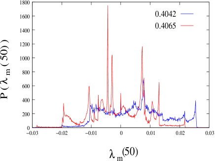
Figure  4.: (Color Online)The probability distribution of the finite time Lyapunov exponents for $t=50$ for the pre-crisis ($\gamma=0.4065$, red colour) region and the postcrisis ($\gamma=0.4042$, blue colour) parameter values. The FTLE-s are equally distributed about zero in the precrisis case indicating the presence of UDV in the region.

5. Conclusion

The embedded standard map is used to model the inertial particle dynamics in a $2-d$ incompressible flow. We concentrate on the dynamical behaviour in the aerosol region. A crisis is seen in in the bifurcation diagram and the largest Lyapunov exponent plot identifies the precise value of $\gamma$ at which the crisis occurs. The statistics of characteristic times between the bursts corresponding to the crisis induced intermittency, behaves as a power law with the exponent $\beta=-1/3$.

The fluctuation of the largest Lyapunov exponent $\lambda_{max}$ around zero, in the neighbourhood of the crisis in the precrisis region, indicates the possibility of the existence of unstable dimension variability in the system. Further, the finite time Lyapunov exponent distribution in the precrisis and the postcrisis scenarios, confirms the presence of UDV in the precrisis region. Thus the shadowing times for the embedded map are expected to be short near the crisis. The implications of this for the dynamics of inertial particles deserve to be explored further. The consequences for aerosols, as in the present study, can be of interest in realistic application contexts. We hope to study these consequences, as well as the role of unstable periodic orbits in the UDV in future work.

REFERENCES

- [1] A.E. Motter, Y.C. Lai, and C. Grebogi, Phys. Rev. E 68, 056307(2003).
- [2] R. Reigada, F. Sagues,J.M. Sancho, Phys. Rev. E 64, 026307(2001).
- [3] A. Babiano, J.H.E. Cartwright, O. Piro, and A. Provenzale, Phys. Rev. Lett 84, 2004.
- [4] N.N. Thyagu and N. Gupte, Phys. Rev. E 76, 046218 (2007).
- [5] Similar results are seen for single initial conditions, including the single initial condition used for plotting the bifurcation diagram.
- [6] R.L. Viana,S.E. de .S. Pinto and C. Grebogi, Phys. Rev. E 66, 046213 (2002).
- [7] R.F. Pereira, S.E. de S.Pinto, R.L. Viana, S.R. Lopes and C. Grebogi, Chaos 17,023131 (2007).
- [8] Y.C. Lai, D. Lerner, K. Williams and C. Grebogi, Phys. Rev. E 60, 5445 (1999).
- [9] Y. Do and Y.C. Lai , Phys. Rev. E 69, 016213 (2004).