Random Dispersion Approximation for the Hubbard model

Abstract

We use the Random Dispersion Approximation (RDA) to study the Mott-Hubbard transition in the Hubbard model at half band filling. The RDA becomes exact for the Hubbard model in infinite dimensions. We implement the RDA on finite chains and employ the Lanczos exact diagonalization method in real space to calculate the ground-state energy, the average double occupancy, the charge gap, the momentum distribution, and the quasi-particle weight. We find a satisfactory agreement with perturbative results in the weak- and strong-coupling limits. A straightforward extrapolation of the RDA data for $L\leq 14$ lattice results in a continuous Mott-Hubbard transition at $U_{\rm c}\approx W$. We discuss the significance of a possible signature of a coexistence region between insulating and metallic ground states in the RDA that would correspond to the scenario of a discontinuous Mott-Hubbard transition as found in numerical investigations of the Dynamical Mean-Field Theory for the Hubbard model.

1 Introduction

The Hubbard model is the minimal lattice model of spin-1/2 electrons that can describe the transition from a metal to a correlated-electron insulator. Long before the formal introduction of the model, Mott Mottbook used a single-band picture to illustrate his idea that, at half band filling and above some critical strength of the mutual Coulomb interaction of the electrons, the ground state must be an insulator with a finite gap for single-electron excitations.

This Mott gap is readily understood in the atomic limit where every lattice site is singly occupied. An additional electron must create a double occupancy, which increases the energy of the ground state by a finite amount $U$, the Mott gap in the atomic limit. For itinerant electrons with bandwidth $W$ and in the strong-coupling limit, $U\gg W$, adding a hole gives rise to the lower Hubbard band of width $W_{\rm hole}\approx W$ in the single-particle density of states. Adding an electron leads to the upper Hubbard band of width $W_{\rm double}\approx W$, so that the Mott gap is of the order of $\Delta=U-W>0$. As $U/W$ becomes smaller, one expects a Mott transition at around $U_{\rm c}\approx W$. Note that this is a genuine quantum phase transition Gebhardbook ; Sachdevbook in the sense that no symmetry breaking needs to occur at $U_{\rm c}$ to change the transport properties from insulating to metallic.

These qualitative arguments do not, however, determine the precise value of the critical interaction strength, the size of the gap, or the Landau quasi-particle weight as a function of the interaction strength. Even the nature of transition is not clear: are the quasi-particle weight and the gap continuous functions of $U/W$ or do they display jump discontinuities at the Mott-Hubbard transition? Since the transition is fundamentally non-perturbative, only exact solutions can answer such questions definitely.

Exact solutions of interacting-electron problems are scarce. The Hubbard model in one dimension Fabianbook displays a Kosterlitz-Thouless-type transition because the Fermi-gas ground state is unstable against an infinitesimal Coulomb interaction, $U_{\rm c}=0^{+}$. This nesting instability is avoided in the chiral or $1/r$-Hubbard model GebhardRuckenstein , and a continuous transition is observed: the discontinuity of the momentum distribution goes to zero when the gap opens linearly above $U_{\rm c}=W$. Thus far, the Hubbard model could not be solved exactly in any dimension $d>1$.

More insight into the Mott-Hubbard transition can be gained in the limit of high dimensions or large lattice coordination number MV ; MHa . In this limit, the Hubbard model can be mapped onto a single-impurity problem in a bath of fermionic particles whose properties must be determined self-consistently (Dynamical Mean-Field Theory, DMFT) Jarrell ; RMP . The single-particle density of states for the corresponding single-impurity problem cannot be obtained analytically.

An alternative is to treat the Hubbard model with a random dispersion relation. The Random Dispersion Approximation (RDA) describes the paramagnetic phase of the Hubbard model in infinite dimensions Gebhardbook ; RDA . The RDA to the Hubbard model cannot be carried out analytically either, i.e., numerical calculations on finite-size systems are necessary to obtain definite results.

Unfortunately, the DMFT and the RDA approaches to the Hubbard model in infinite dimensions give conflicting scenarios for the Mott-Hubbard transition. All numerical studies of the DMFT equations favor a discontinuous transition with a jump discontinuity in the gap, whereas the RDA results favor a continuous transition.

In this work, we present numerical results for the Random Dispersion Approximation to the Hubbard model. In Section 2 we introduce the Hubbard model, formulate the RDA approach, and give a simple example of finite-size effects within the RDA. In Section 3, we give the RDA results for the ground-state energy, the single-particle gap, the quasi-particle weight, and other physical quantities in the infinite-dimensional Hubbard model. In Section 4, we critically discuss the two scenarios for the Mott-Hubbard transition and try to reconcile the conflicting results. A short conclusion, Section 5, closes our presentation.

2 Random Dispersion Approximation for the Hubbard model

We start our presentation with the definition of the Hubbard Hamiltonian. Next, we formulate the Random Dispersion Approximation (RDA) for the Hubbard model which becomes exact in the limit of infinite lattice coordination number. Finally, we illustrate the RDA by calculating the ground-state energy to second order in weak-coupling perturbation theory.

2.1 Hubbard Hamiltonian

We investigate spin-1/2 electrons on a lattice. Their motion is described by

$$\hat{T}=\sum_{\vec{i},\vec{j};\sigma}t_{\vec{i},\vec{j}}\hat{c}_{\vec{i},\sigma}^{\dagger}\hat{c}_{\vec{j},\sigma}^{\vphantom{\dagger}}\;,$$ (1)

where $\hat{c}^{\dagger}_{\vec{i},\sigma}$, $\hat{c}_{\vec{i},\sigma}^{\vphantom{\dagger}}$ are creation and annihilation operators for electrons with spin $\sigma=\uparrow,\downarrow$ on site $\vec{i}$. Here the $t_{\vec{i},\vec{j}}$ are the electron transfer amplitudes between sites $\vec{i}$ and $\vec{j}$, and $t_{\vec{i},\vec{i}}=0$.

For lattices with translational symmetry, we have $t_{\vec{i},\vec{j}}=t(\vec{i}-\vec{j})$, and the operator for the kinetic energy is diagonal in momentum space,

$$\hat{T} = \sum_{\vec{k};\sigma}\epsilon(\vec{k})\hat{c}^{\dagger}_{\vec{k},\sigma}\hat{c}_{\vec{k},\sigma}^{\vphantom{\dagger}}\;,$$

$$\epsilon(\vec{k}) = \frac{1}{L}\sum_{\vec{m},\vec{j}}t(\vec{m}-\vec{j})e^{-{\rm i}(\vec{m}-\vec{j})\vec{k}}\;,$$ (2)

where $\epsilon(\vec{k})$ is the dispersion relation. The electrons are assumed to interact only locally, and the Hubbard interaction reads

$$\hat{D}=\sum_{\vec{i}}\hat{n}_{\vec{i},\uparrow}\hat{n}_{\vec{i},\downarrow}\;,$$ (3)

where $\hat{n}_{\vec{i},\sigma}=\hat{c}^{\dagger}_{\vec{i},\sigma}\hat{c}_{\vec{i},\sigma}^{\vphantom{\dagger}}$ is the local density operator at site $\vec{i}$ for spin $\sigma$. This leads to the Hubbard model HubbardI ,

$$\hat{H}=\hat{T}+U\hat{D}\;.$$ (4)

Since we are ultimately interested in the Mott-Hubbard transition, we consider a half-filled band exclusively, i.e., a number of electrons $N$ that equals the number of lattice sites $L$ (even). Furthermore, we consider only the paramagnetic phase with $N_{\uparrow}=N_{\downarrow}=L/2$ electrons.

2.2 Formulation of the approximation

2.2.1 Hubbard model with a random dispersion relation

The density of states for non-interacting electrons is given by

$$\rho(\epsilon)=\frac{1}{L}\sum_{\vec{k}}\delta(\epsilon-\epsilon(\vec{k}))\;.$$ (5)

In the limit of high lattice dimensions and for translationally invariant systems, the Hubbard model is characterized by $\rho(\epsilon)$ alone, i.e., higher-order correlation functions in momentum space factorize, e.g., PvDetal

$$\rho_{\vec{q}_{1},\vec{q}_{2}}(\epsilon_{1},\epsilon_{2}) \equiv \frac{1}{L}\sum_{\vec{k}}\delta\bigl{(}\epsilon_{1}-\epsilon(\vec{k}+\vec{q}_{1})\bigr{)}\delta\bigl{(}\epsilon_{2}-\epsilon(\vec{k}+\vec{q}_{2})\bigr{)}$$

$$= \rho(\epsilon_{1})[\delta_{\vec{q}_{1},\vec{q}_{2}}\delta(\epsilon_{1}-\epsilon_{2})+(1-\delta_{\vec{q}_{1},\vec{q}_{2}})\rho(\epsilon_{2})]\,.$$

This is the characteristic property of the dispersion relation in infinite dimensions Gebhardbook ; RDA .

In the Random Dispersion Approximation, the dispersion relation $\epsilon(\vec{k})$ of the Hubbard model in (2) is replaced by a random dispersion relation $\epsilon^{\rm RDA}(\vec{k})$, where each $\vec{k}$ point of the Brillouin zone is randomly assigned a kinetic energy from the probability distribution $\rho(\epsilon)$, the bare density of states in (5). As has been shown earlier Gebhardbook ; RDA , the RDA for the Hubbard model is equivalent to the exact solution of the Hubbard model in infinite lattice dimensions MV ; MHa ; RMP when long-range order is absent.

When we choose a semi-ellipse as our bare density of states, the RDA for the Hubbard model becomes exact on a Bethe lattice with infinite coordination number Economou ,

$$\rho_{0}(\epsilon)=\frac{4}{\pi W}\sqrt{1-\left(\frac{2\epsilon}{W}\right)^{2}\,}\quad,\quad(|\epsilon|\leq W/2)\;,$$ (7)

where $W\equiv 4t$ is the bare bandwidth. In the following, we shall use $t\equiv 1$ as our energy unit.

2.2.2 Implementation on finite systems

In order to put the RDA into practice, we must calculate physical quantities for various realizations ${\cal Q}$ of the dispersion relation and system sizes $L$, i.e., we must calculate expectation values

$$X_{\cal Q}(L)={}_{\cal Q}\langle\Psi_{0}(L)|\hat{X}|\Psi_{0}(L)\rangle_{\cal Q}$$ (8)

for observables $\hat{X}$ in the ground state $|\Psi_{0}(L)\rangle_{\cal Q}$ of $\hat{H}_{\cal Q}(L)$. Physically meaningful quantities are obtained by averaging over a large number $R_{L}$ of realizations and extrapolating to the thermodynamic limit,

$$X=\lim_{L\to\infty}\frac{1}{R_{L}}\sum_{\cal Q}X_{\cal Q}(L)\;.$$ (9)

Typically, we choose $R_{L}=1000$ for $6\leq L\leq 14$. For distributions with a Gaussian form, we can determine the average values with accuracy ${\cal O}(1/L)$. The accessible system size is the limiting factor in the RDA.

We choose anti-periodic boundary conditions for even $L$ lattice sites in momentum space

$$k=\frac{\pi}{L}\left(-L-1+2m\right)\quad,\quad m=1,2,\ldots,L\;,$$ (10)

and determine the dispersion relation $\epsilon(k)$ as the solution of the implicit equation

$$k=\frac{4\epsilon(k)}{W}\sqrt{1-\left(\frac{2\epsilon(k)}{W}\right)^{2}\,}+2\arcsin\left(\frac{2\epsilon(k)}{W}\right)\;.$$ (11)

This choice guarantees that we recover $\rho_{0}(\epsilon)$ from $\epsilon(k)$ in the thermodynamic limit. Next, we choose a permutation ${\cal Q}_{\sigma}$ for each spin direction $\sigma$ that permutes the sequence $\{1,\ldots,L\}$ into $\{{\cal Q}_{\sigma}[1],\ldots,{\cal Q}_{\sigma}[L]\}$. This defines a realization of the RDA dispersion, ${\cal Q}=[{\cal Q}_{\uparrow},{\cal Q}_{\downarrow}]$. The numerical task is the Lanczos diagonalization of the Hamiltonian

$$\hat{H}_{{\cal Q}}(L)=\sum_{\sigma}\sum_{\ell=1}^{L}\epsilon(k_{{\cal Q}_{\sigma}[\ell]})\hat{c}_{k_{\ell},\sigma}^{\dagger}\hat{c}_{k_{\ell},\sigma}^{\vphantom{\dagger}}+U\hat{D}\;.$$ (12)

In this way, we obtain, e.g., the momentum distribution for a realization

$$n_{\cal Q}(\epsilon;L)=\frac{1}{2}\sum_{\sigma}\left.{}_{\cal Q}\langle\Psi_{0}(L)|\hat{n}_{k_{\ell},\sigma}|\Psi_{0}(L)\rangle_{\cal Q}\right|_{\epsilon(k_{\ell})=\epsilon}\;,$$ (13)

which depends on momentum $\vec{k}$ only via the dispersion relation $\epsilon(\vec{k})$ MV ; MHa (and depends on the realization ${\cal Q}$).

2.3 Second-order ground-state energy in the RDA

As an example, we calculate the ground-state energy $E=\langle\hat{H}\rangle$ to second order in the interaction strength numerically. Within the RDA we have (${\cal Q}=\left[{\cal Q}_{\uparrow}{\cal Q}_{\downarrow}\right]$)

$$E_{{\cal Q}_{\uparrow}{\cal Q}_{\downarrow}}(U;L)=E^{(0)}(L)+\frac{UL}{4}+U^{2}E^{(2)}_{{\cal Q}_{\uparrow}{\cal Q}_{\downarrow}}(L)+\ldots\;,$$ (14)

where $E^{(0)}(L)$ is the ground-state energy of the Fermi sea, which is independent of the configuration ${\cal Q}$. $E^{(2)}_{{\cal Q}_{\uparrow}{\cal Q}_{\downarrow}}(L)$ is the leading correction, which is obtained from Rayleigh-Schrödinger perturbation theory as

$$\frac{E^{(2)}_{{\cal Q}_{\uparrow}{\cal Q}_{\downarrow}}(L)}{L} = -\left(\frac{1}{L}\right)^{3}\sum_{|k|<\pi}\Theta(-\epsilon_{{\cal Q}_{\uparrow}}(k))\sum_{|p|<\pi}\Theta(-\epsilon_{{\cal Q}_{\downarrow}}(p))$$

$$\sum_{0<q<2\pi}\frac{\Theta(\epsilon_{{\cal Q}_{\uparrow}}(k+q))\Theta(\epsilon_{{\cal Q}_{\downarrow}}(p-q))}{\epsilon_{{\cal Q}_{\uparrow}}(k+q)-\epsilon_{{\cal Q}_{\uparrow}}(k)+\epsilon_{{\cal Q}_{\downarrow}}(p-q)-\epsilon_{{\cal Q}_{\downarrow}}(p)}\;,$$

where $\Theta(x)$ is the Heaviside step function. Here $p-q$ and $k+q$ must lie in the first Brillouin zone, i.e., $p-q\equiv p-q\ {\rm mod}\ 2\pi$, $k+q\equiv p+q\ {\rm mod}\ 2\pi$, with

$$k = \frac{\pi}{L}\left(-L+1+2\ell\right)\quad;\quad\ell=0,\ \ldots,\ L-1\;,$$

$$p = \frac{\pi}{L}\left(-L+1+2m\right)\quad;\quad m=0,\ \ldots,\ L-1\;,$$

$$q = \frac{2\pi n}{L}\quad;\quad n=1,\ \ldots,\ L-1\;.$$ (16)

In order to illustrate the importance of finite-size effects in the RDA, we plot histograms of the RDA data for $E^{(2)}_{{\cal Q}_{\uparrow}{\cal Q}_{\downarrow}}(L)$ for $N_{L}=10000$ configurations and $L=12$, $20$, $128$, and $256$ in Fig. 1.

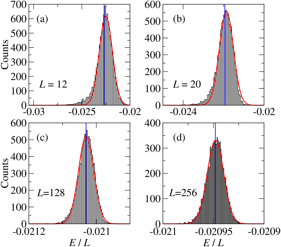
Figure 1: Histograms of the second-order correction $E^{(2)}_{{\cal Q}_{\uparrow}{\cal Q}_{\downarrow}}(L)$ to the ground-state energy in weak coupling for (a) $L=12$, (b) $L=20$, (c) $L=128$, and (d) $L=256$ sites. The lines give the mean values of the RDA histograms, and the curves are fits to the Gaussian function $f(E/L)=a(L)\exp[-(E/L-b(L))^{2}/(2c(L)^{2})]$.

A closer analysis of Eq. (LABEL:eqn:E2) shows that the histograms for $E^{(2)}_{{\cal Q}_{\uparrow}{\cal Q}_{\downarrow}}(L)$ become Gaussian for large system sizes and that their width shrinks proportionally to $1/L$. For $L<100$, the histograms are not perfectly Gaussian yet, introducing a small systematic error in the mean value for a given system size. Nevertheless, the mean value can be determined with an accuracy that is a factor of $1/L$ better than the width of the distribution, $c(L)$. The finite-size extrapolation of the second-order correction $E^{(2)}(L)$ is shown in Fig. 2.

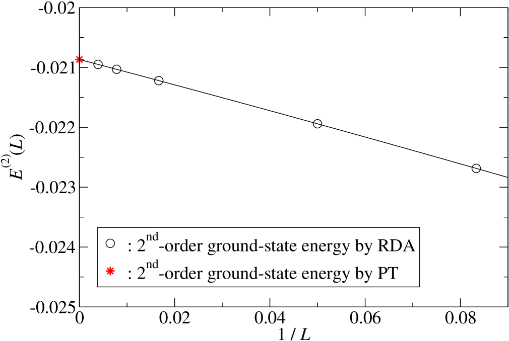
Figure 2: Finite-size extrapolation of the second-order correction $E^{(2)}(L)$ to the ground-state energy in weak coupling. The line is a second-order polynomial in $1/L$. The star marks the analytic result in the thermodynamic limit, see Eq. (18).

As seen from the figure, the RDA perfectly reproduces the result from Rayleigh-Schrödinger perturbation theory for the Hubbard model in Eq. (18), see below. From the RDA with $L\leq 256$, we find $E^{(2),L\leq 256}=-0.0208661(9)$, compared to the analytic result $E^{(2)}=-0.02086614838$. Even if we take only the results for $L=12$ and $L=20$ into account, a fairly accurate estimate can be obtained, $E^{(2),L\leq 20}=-0.0208(2)$.

However, outside the perturbative limit, even $L=20$ is beyond our numerical capabilities. The RDA calculations which we present in the rest of this work are based on the exact diagonalization (ED) method which is limited to $L\leq 14$ lattice sites because of the memory capacity. Calculations for $L=16$ sites using our ED code requires about 33 GB memory. Therefore, numerical calculations for $R_{L}=1000$ configurations are prohibitively expensive.

In principle, larger systems can be treated using the Density-Matrix Renormalization Group (DMRG). However, the nonlocal nature of the hopping makes the problem difficult in real space, and the nonlocal nature of the interaction in momentum space makes the problem difficult in reciprocal space Nishimoto-kspace . Therefore, the maximum system size that can be treated reliably using the DMRG is, at present, only marginally larger than the $L=14$ treated here.

3 Physical quantities

In this section, we present RDA data for the ground-state energy, the average double occupancy, the charge gap, the momentum distribution, and the quasi-particle weight. We compare our results with those from perturbation theory in weak and strong coupling and from numerical approaches to the Hubbard model in infinite dimensions (Quantum Monte Carlo, the Dynamical DMRG, and the Numerical Renormalization Group).

3.1 Energy and double occupancy

The ground-state energy per site $E(U)/L$ and the average double occupancy $d(U)$ are related by

$$d(U)=\frac{1}{L}\langle\hat{D}\rangle=\frac{1}{L}\frac{\partial E(U)}{\partial U}\;.$$ (17)

In weak coupling, the ground-state energy was calculated to fourth-order using the Brueckner–Goldstone perturbation theory Ruhl ,

$$\frac{E(U)}{L} = -\frac{8}{3\pi}+\frac{U}{4}-0.02086614838\,U^{2}$$ (18)

$$+0.0000072475\,U^{4}+{\cal O}\left(U^{6}\right)\;,$$

$$d(U) = \frac{1}{4}-0.04173229676\,U$$ (19)

$$+0.00002899\,U^{3}+{\cal O}\left(U^{5}\right)\;.$$

In strong coupling, a diagrammatic approach based on the Kato–Takahashi perturbation theory provides the results to 11th order EvaFlorian ; NilsEva ,

$$\frac{E(U)}{L} = -\frac{1}{2U}-\frac{1}{2U^{3}}-\frac{19}{8U^{5}}-\frac{593}{32U^{7}}$$ (20)

$$-\frac{23877}{128U^{9}}-\frac{4496245}{2048U^{11}}-{\cal O}(U^{-13})\;,$$

$$d(U) = \frac{1}{2U^{2}}+\frac{3}{2U^{4}}+\frac{95}{8U^{6}}+\frac{4151}{32U^{8}}+\frac{214893}{128U^{10}}$$ (21)

$$+\frac{49458695}{2048U^{12}}+{\cal O}(U^{-14})\;.$$

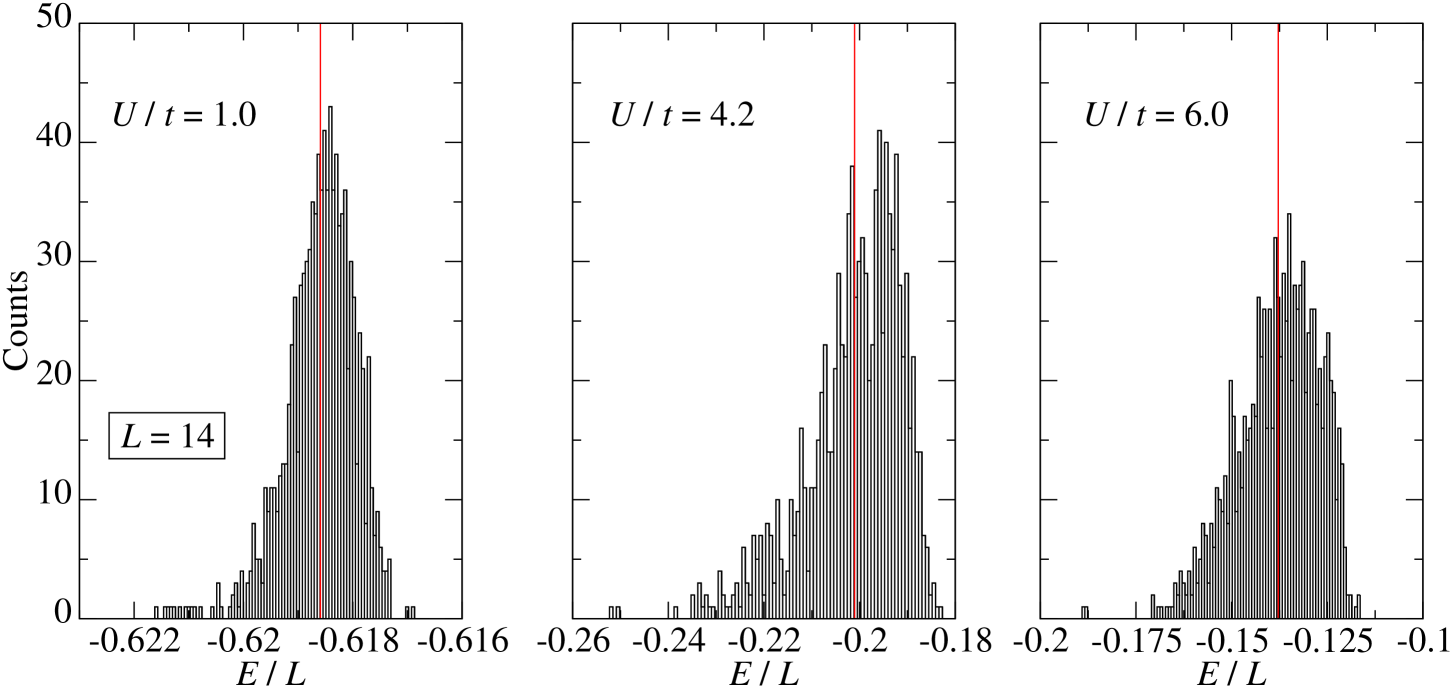
Figure 3: Histograms of the ground-state energy for $U/t=1$ (left), $U/t=4.2$ (middle), and $U/t=6$ (right) for $L=14$ (bandwidth $W/t=4$). The lines indicate the mean values.

In Fig. 3, we show three histograms of the ground-state energy distribution for $U/t=1$, $U/t=4.2$, and $U/t=6$ (bandwidth $W/t=4$) for $L=14$, calculated using ED with the RDA. The lines indicate the mean values. In the weak-coupling regime, the histograms are rather symmetric and the relative width of the distribution is quite small, so that the finite-size error is also small in this parameter regime. In strong coupling, on the other hand, the histograms are fairly asymmetric and their relative width is much broader than in the weak-coupling region. Therefore, the finite-size effects are much larger and the extrapolated data are less accurate than in the weak-coupling regime. The inset of Fig. 4 shows the finite-size-scaling analysis of the ground-state energy for various interaction strengths. The finite-size dependence of the average values is weak, so that reasonable estimates for the ground-state energy can be obtained from the extrapolation of small system sizes.

Figure 4: Extrapolated data for the ground-state energy as a function of the interaction strength in the RDA (circles), the DDMRG for a metallic solution (open triangles) Nishim , the DDMRG for an insulating solution (filled triangles) Nishim3 , QMC (stars) NilsEva ; NilsQMC , weak-coupling perturbation theory [Eq. (18)] (solid line) Ruhl , and strong-coupling perturbation theory [Eq. (20)] (dotted line) NilsEva . Inset: ground-state energy as a function of inverse system size ($L\leq 14$) in the RDA for various interaction strengths.

In Fig. 4, we also compare the extrapolated RDA results as a function of the interaction strength $U/t$ with those from Quantum Monte-Carlo (QMC) NilsEva ; NilsQMC , the Dynamical Density-Matrix Renormalization Group method (DDMRG) Nishim ; Nishim3 , weak-coupling perturbation theory, see Eq. (18) Ruhl , and strong-coupling perturbation theory, see Eq. (20) NilsEva . As expected from the histograms and from the extrapolation of the ground-state energy, the RDA results agree very well with those from all other methods in the weak-coupling regime. However, for $U\geq W$ the agreement is worse, as the ground-state energy extrapolated from the RDA is consistently lower than the ground-state energy obtained from the DDMRG, QMC, and the strong-coupling expansion.

In Fig. 5, we show the histograms for the double occupancy for $L=14$ sites and $U/t=1$, $U/t=4.2$, and $U/t=6$ (with bandwidth $W/t=4$). As for the ground-state energy, the histograms are fairly narrow for small interaction strengths and are rather broad for large coupling. Correspondingly, the extrapolated data are more reliable for small than for large interaction. Interestingly, a double-peak structure appears for $U\approx W$. This could be a signature of two coexisting solutions for intermediate interaction strengths RMP . We shall further discuss the significance of this structure in Section 4.

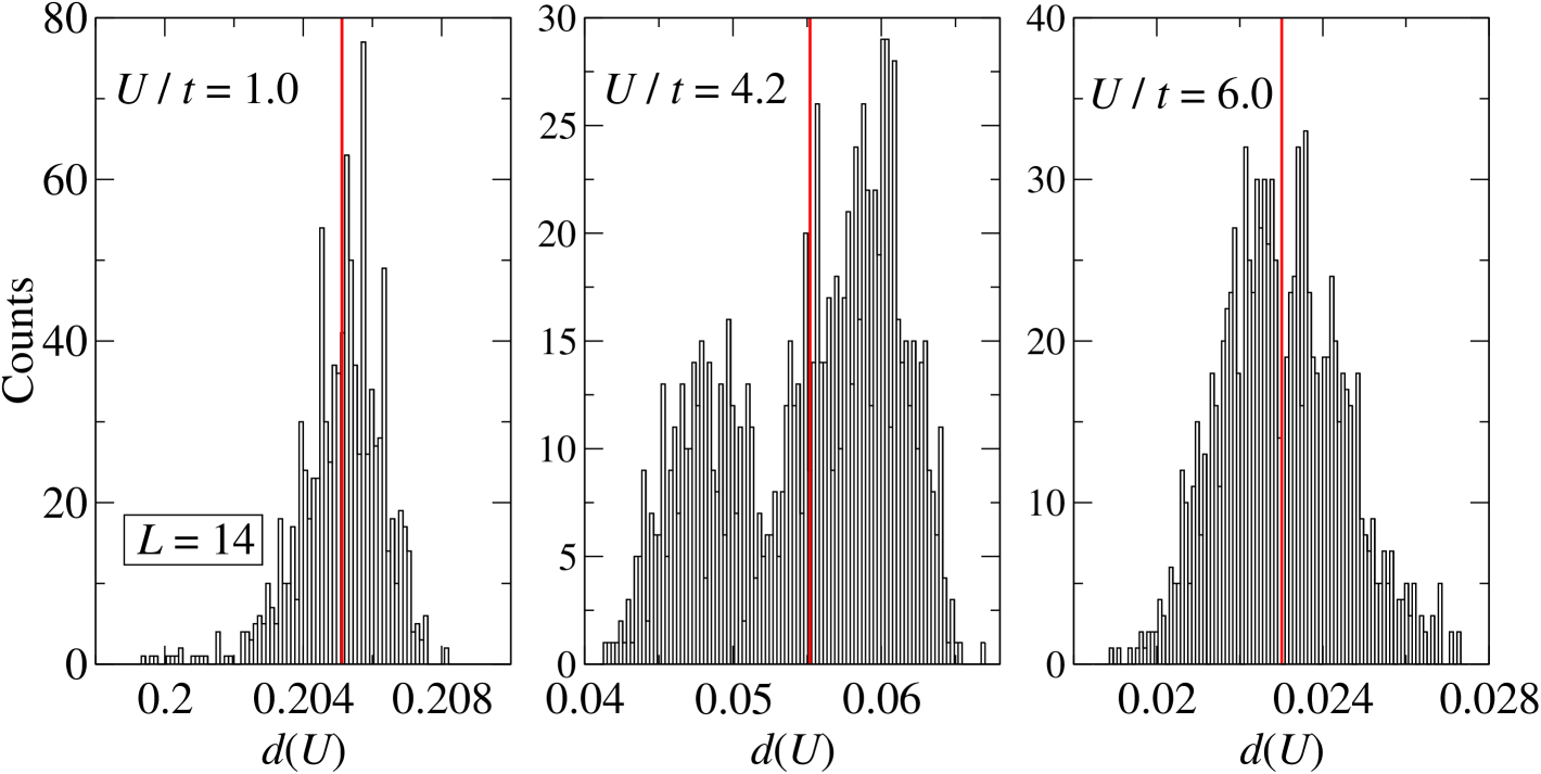
Figure 5: Histograms of the double occupancy in the RDA for interaction strengths $U/t=1$ (left), $U/t=4.2$ (middle), and $U/t=6$ (right) for $L=14$ (bandwidth $W/t=4$). The lines indicate the mean values.

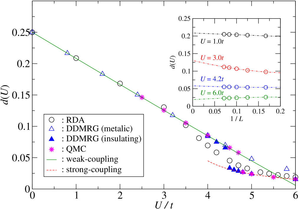
Figure 6: Extrapolated data for the double occupancy as a function of the interaction strength in the RDA (circles), the DDMRG for a metallic solution (open triangles) Nishim , the DDMRG for an insulating solution (filled triangles) Nishim3 , QMC (stars) NilsEva ; NilsQMC , weak-coupling perturbation theory [Eq. (19)] (solid line) Ruhl , and strong-coupling theory [Eq. (21)] (dotted line) NilsEva . Inset: double occupancy as a function of the inverse system size for $L\leq 14$ in the RDA for various values of the interaction strengths.

We now extrapolate the mean value of the double occupancy as prescribed in Eq. (9). We show the resulting data for the double occupancy in Fig. 6, where we compare our results with those from QMC NilsEva ; NilsQMC , the DDMRG Nishim ; Nishim3 , weak-coupling perturbation theory, see Eq. (19) Ruhl , and strong-coupling perturbation theory, see Eq. (21) NilsEva . Again, the RDA reproduces the weak-coupling expression very well, and also provides a reasonable description of the strong-coupling limit. In the transition region, $3.5\leq U\leq 5$, the RDA result for the double occupancy smoothly interpolates between the DDMRG and the QMC results for the metallic phase and the insulating phase. For a further discussion, see Section 4.

3.2 Charge gap

We calculate the single-particle gap,

$$\Delta_{\cal Q}(U;L)=E_{\cal Q}(U;L+1)+E_{\cal Q}(U;L-1)-2E_{\cal Q}(U;L)$$ (22)

for each configuration ${\cal Q}$, where $E_{\cal Q}(U;N)$ is the ground-state energy for a system with $N$ particles. From the strong-coupling theory EvaFlorian , the charge gap in the thermodynamic limit is obtained as

$$\Delta(U)=U-4-\frac{1}{U}-\frac{3}{2U^{2}}+{\cal O}\left(\frac{1}{U^{3}}\right)\;.$$ (23)

Again, the histograms for the charge gap are fairly broad. We mention in passing that the ground-state momenta for different particle numbers are not necessarily the same.

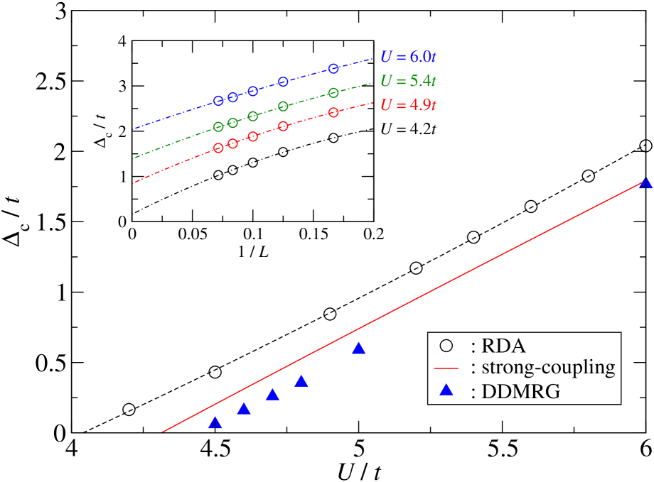
Figure 7: Extrapolated data for the single-particle gap as a function of the interaction strength $U$ in the RDA (circles), the DDMRG for an insulating solution (triangles) Nishim , and the second-order strong-coupling expansion [Eq. (23)] (solid line) EvaFlorian . Inset: single-particle gap as a function of the inverse system size ($L\leq 14$) in the RDA for various values of the interaction strengths.

In Fig. 7, we compare the RDA results with the predictions from DDMRG Nishim and the strong-coupling expansion. Evidently, the RDA extrapolation from data for small systems ($L\leq 14$) overestimates the size of the gap and underestimates the stability of the metallic solution. Therefore, the RDA predicts a insulator-to-metal transition at $U\approx W$ RDA .

3.3 Momentum distribution and quasi-particle weight

In the limit of infinite dimensions MV ; MHa and within the RDA, the momentum distribution depends on $\vec{k}$ through the bare dispersion relation $\epsilon(\vec{k})$ only, see Eq. (13).

In Fig. 8, we show the results for the momentum distribution for weak to intermediate couplings. For $U\leq W/2=2$, we find very good agreement between the results from the RDA and those from weak-coupling perturbation theory to fourth order in the interaction strength. It is known from Feynman-Dyson perturbation theory SandraFlorian that the fourth-order expression becomes unreliable for $U>0.6W=2.4$. Therefore, we do not plot the perturbative result for $U=W$.

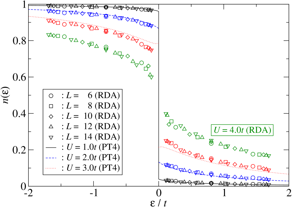
Figure 8: RDA data for the momentum distribution for various system sizes and interaction strengths $U/t=1,2,3,4$ (symbols) in comparison with the results from weak-coupling perturbation theory Ruhl (lines).

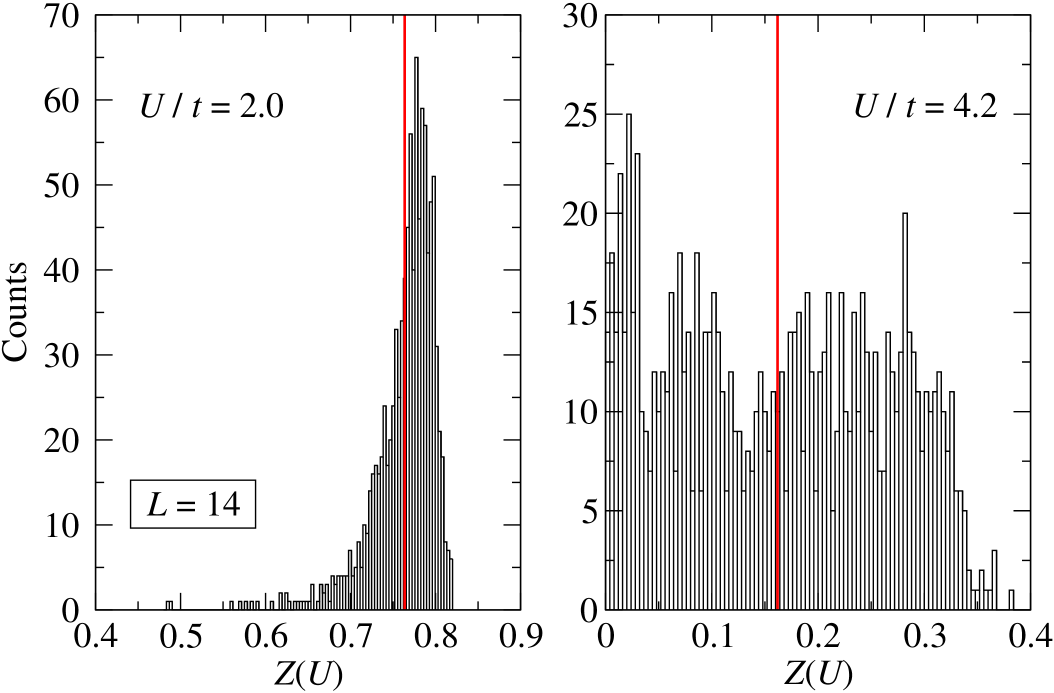
Figure 9: Histograms for the quasi-particle weight for $U/t=2$ (left) and $U/t=4.2$ (right) for $L=14$ sites. The long vertical lines indicate the mean values of the RDA histograms.

Fig. 8 shows that the finite-size effects are strongest close to the Fermi energy, $E_{\rm F}=0$. Consequently, a reliable calculation of the size of the jump discontinuity at $E_{\rm F}$ is difficult. Since the self-energy is independent of momentum MV ; MHa ; RMP , the quasi-particle weight is obtained from

$$Z_{\cal Q} = n_{\cal Q}(\epsilon=0^{-})-n_{\cal Q}(\epsilon=0^{+})$$ (24)

$$= 2n_{\cal Q}(\epsilon=0^{-})-1\;,$$

where the second line follows from particle-hole symmetry. For finite system sizes, we approximate the quasi-particle weight by the difference of the momentum distributions at $k=\pm\pi/L$ which are closest to $\epsilon=E_{\rm F}=0$,

$$Z_{\cal Q}(U;L)=2n_{\cal Q}\left(\epsilon(-\pi/L)\right)-1\;,$$ (25)

and then extrapolate to the thermodynamic limit. The Brueckner-Goldstone Ruhl and Feynman-Dyson SandraFlorian perturbation theories give the following result to fourth order in the interaction strength,

$$Z(U)=1-0.0817484\,U^{2}+0.00380158\,U^{4}+{\cal O}\left(U^{6}\right)\;.$$ (26)

This expression can be used for $U\leq 0.6W=2.4$ SandraFlorian .

In Fig. 9 we show the histograms for the quasi-particle weight for $U/t=2$ and $U/t=4.2$ for $L=14$ sites. For small interaction strengths, the histograms show a fairly narrow peak, and the mean value is well defined. For interaction strengths close to the metal-insulator transition, the distribution is broad because, for finite systems, even an ‘insulating’ configuration has a finite jump in the momentum distribution, $Z(L;U\gg W)={\cal O}(W/(LU))$. Therefore, we expect $Z_{\cal Q}(L;U/t=4.2)={\cal O}(1/L)$ which gives $Z_{\cal Q}(L=14;U/t=4)\approx 0.07$ for our system size. Therefore, at intermediate to large coupling strengths, the finite-size effects for the quasi-particle weight are quite large.

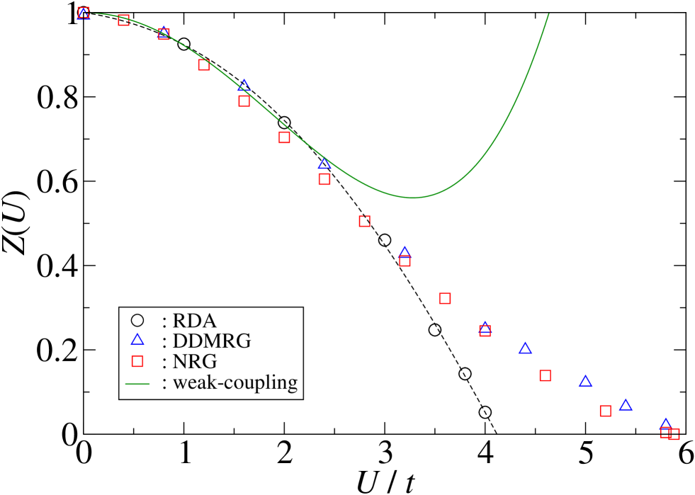
Figure 10: Extrapolated data for the quasi-particle weight as a function of the interaction strength in the RDA (circles), the DDMRG for a metallic solution (triangles) Nishim , the NRG (squares) RBulla , and fourth-order weak-coupling perturbation theory [Eq. (26)] Ruhl ; SandraFlorian (solid line). The dotted line is a guide to the eye only.

In Fig. 10 we compare the extrapolated RDA results with the predictions from DDMRG Nishim , NRG RBulla and the weak-coupling expansion Ruhl ; SandraFlorian . Evidently, the RDA extrapolation for $Z(U)$ from the data for small systems ($L\leq 14$) agrees very well with all other methods for $U\leq 3$. For $U>3$, the RDA quasi-particle weight goes down quickly and vanishes at $U_{\rm c}\approx W$, where the gap opens RDA . All other methods used for the solution of the Dynamical Mean-Field Theory for the Hubbard model find metallic solutions which exist up to $U_{{\rm c},2}\approx 1.5W=6$.

We shall discuss these contrasting findings in the next section.

4 Discussion

We first lay out the two conflicting scenarios for the Mott-Hubbard transition in the Hubbard model with infinite coordination number. The RDA results suggest a continuous transition, whereas numerical treatments of the self-consistency equations from the Dynamical Mean-Field Theory support a discontinuous transition. We discuss objections to this scenario as well as possible remedies. Finally, we re-analyze the RDA results of Section 3 for signatures of coexistence of metallic and insulating ground states.

4.1 Scenarios for the Mott transition

Within the RDA or in the limit of large coordination number, the metallic phase is marked by a finite quasi-particle weight $Z(U)$, while a finite gap for single-particle excitations $\Delta(U)$ characterizes the Mott-Hubbard insulator. Within the limits of the accuracy of the extrapolation, the RDA predicts the Mott transition to be continuous: as a function of the interaction strength $U$, the quasi-particle weight goes to zero at $U_{\rm c}\approx W$, where the gap opens. All thermodynamic quantities, such as the ground-state energy and the average double occupancy, are continuous functions of the interaction strength $U$.

The scenario of a continuous transition is in conflict with the prediction of a discontinuous transition, as has been obtained from numerical solutions of the self-consistency equations in the Dynamical Mean-Field Theory (DMFT) RMP . A metallic solution is found for $0\leq U\leq U_{{\rm c},2}\approx 5.9\ldots 6.2$, whereas an insulating solution exists for $U_{{\rm c},1}\approx 4.5\ldots 4.8\leq U$; the precise values for $U_{{\rm c},1}$ and $U_{{\rm c},2}$ are still under discussion EvaFlorian ; NilsEva ; RBulla ; Nishim2 ; Uhrig . Since the metallic solution is found to be lower in energy than the insulating solution, the metal-to-insulator transition occurs at $U_{\rm c}=U_{{\rm c},2}$ so that the quasi-particle weight goes to zero continuously but the gap jumps to the pre-formed value associated with the insulating solution.

A finite coexistence region at temperature $T=0$ implies a line of first-order phase transitions in the $(U,T)$ phase diagram below a critical temperature $T_{\rm c}$. It is tempting to apply the latter to explain the phase diagram of V₂O₃ RMP ; physicstoday , which also displays a line of first-order phase transitions between a ‘metallic’ and an ‘insulating’ phase. Note, however, that the vanadium compound shows very large volume changes across the transition so that lattice effects probably dominate the behavior at the transition Krish . Moreover, the critical temperature $T_{\rm c}$ derived from the electronic mechanism alone appears to be too low to account for the experimentally observed critical temperature.

4.2 Problems of the scenario of a discontinuous transition

The scenario of a discontinuous transition has been criticized on mathematical as well as on physical grounds.

4.2.1 Kehrein argument

For $U\to U_{{\rm c},2}^{-}$, the single-particle spectral function of the metallic solution consists of a quasi-particle resonance of width $ZW\ll W$ which is energetically isolated from the lower and upper Hubbard bands, which are split by the pre-formed gap $\Delta_{\rm pre}$. As shown by Kehrein Kehrein , a strict separation of energy scales implies that the self-energy must display a singularity on an intermediate energy scale $ZW\ll\epsilon_{\rm c}=\sqrt{Z}W\ll\Delta_{\rm pre}$. Such a singular behavior of the self-energy is very problematic because the DMFT mapping of the Hubbard model onto an effective single-impurity model is based on the Dyson equation and on the skeleton expansion around the weak-coupling limit. The corresponding resummations of the perturbation series become questionable if the resulting self-energy displays singularities as a function of frequency.

A way out of this dilemma is the concept of a quantum phase transition ‘as a function of frequency’. As shown by Metzner MetznerZPHYS , the DMFT mapping can also be achieved perturbatively starting from the atomic limit. Therefore, one can argue that the weak-coupling perturbation theory converges for all frequencies in the region $0\leq U<U_{{\rm c},1}$ and that the strong-coupling perturbation theory converges for all frequencies in the region $U>U_{{\rm c},2}$. In the coexistence region, $U_{{\rm c},1}<U<U_{{\rm c},2}$, the weak-coupling perturbation theory converges for a finite frequency interval $|\omega|<\epsilon_{\rm c}$, while the strong-coupling perturbation theory converges outside this interval. Therefore, a quantum phase transition ‘as a function of frequency’, signaled by a divergence in the self-energy at $\epsilon_{\rm c}$, is contained in the metallic solution. It becomes a true transition when $Z(U_{{\rm c},2})=\epsilon_{\rm c}(U_{{\rm c},2})=0$ at $U=U_{{\rm c},2}$. Note, however, that this is a justification a posteriori, and it is not clear a priori that numerical methods for the solution of the DMFT self-consistency equation can treat such divergences properly.

Recently, Karski et al. Uhrig proposed that bound states exist in the coexistence regime. In their DDMRG data, they detected signatures of resonances at the edges of the lower and upper Hubbard bands. However, no such resonances are discernible in recent QMC data of Blümer NilsQMC ; see, however, Ref. Jarrell . While the possibility of bound states is not discussed in Kehrein’s analysis, the existence of any kind of singularities in the density of states makes the resummation of the perturbation series disputable.

4.2.2 Logan-Nozières argument

A physical argument which questions the scenario of a discontinuous transition was presented by Logan and Nozières Logan . In the metallic phase close to $U_{{\rm c},2}$, a small number of itinerant electrons, $N_{\rm itin}=ZN$, must screen a large number $N_{\rm loc}=(1-Z)N$ of localized spins. For a regular Kondo screening process with Kondo energy $T_{\rm K}\approx ZW$, the screening energy is gained once per screening electron, i.e., it is of the order $E_{\rm gain}=N_{\rm itin}T_{\rm K}\approx Z^{2}WN$. The itinerant electrons must be excited over the performed gap $\Delta_{\rm pre}$. Therefore, the loss of energy is given by $E_{\rm loss}=N_{\rm itin}\Delta_{\rm pre}=ZN\Delta_{\rm pre}$. Balancing the two energies thus gives $\Delta_{\rm pre}\approx ZW$, i.e., the pre-formed gap and the quasi-particle weight both vanish at a (single) critical $U_{\rm c}$.

This argument does not take into account the possibility that the ‘metallic’ pre-formed gap can be larger than the corresponding gap in the insulating solution. Such a behavior has recently been observed in Ref. Uhrig . Therefore, there is an additional energy gain $E_{\rm low}=ZN\Delta_{\rm pre}$ in the metallic system because the quasi-particle resonance pushes the filled lower Hubbard band downwards in energy by approximately $Z\Delta_{\rm pre}$. This level repulsion, rather than the Kondo screening, may account for the existence of the quasi-particle resonance in the pre-formed gap. Again, this is merely an a posteriori interpretation of the results obtained from numerical solutions of the self-consistency equations in the Dynamical Mean-Field Theory.

4.3 Coexistence of metallic and insulating ground states in the RDA?

Kehrein’s analysis Kehrein points to two basic problems of the DMFT: (i) How many self-consistent solutions exist for $U>0$? (ii) Which of the self-consistent solutions corresponds to the Hubbard model in infinite dimensions?

It is conceivable that multiple ‘metallic’ and ‘insulating’ solutions of the DMFT equations exist. Some of them may easily be detected numerically, others may be elusive. Some solutions ought to be discarded because their analytical properties violate the conditions on which the mapping was based in the first place. Therefore, solutions of the DMFT equations that advocate a continuous Mott-Hubbard transition may be more difficult to find numerically Nishim2 , but they could be relevant.

It is the main advantage of the Random Dispersion Approximation to the Hubbard model that it is not based on a set of self-consistency equations. Therefore, it provides an independent approach to the Hubbard model with infinite coordination number. Unfortunately, the system sizes which we can treat are fairly small, and it is difficult to come to definite conclusions about the existence of a continuous or a discontinuous Mott transition.

As mentioned at the end of Section 3, the RDA predicts a continuous transition at $U_{\rm c}\approx W$ RDA . One may ask if and how the RDA on finite lattices could describe a coexistence region. As a bare ground-state method, in the infinite-system limit it should give a metallic solution for $U<U_{{\rm c},2}$ and an insulating solution with a finite, sizable gap for $U>U_{{\rm c},2}$. The average double occupancy would follow the weak-coupling curve up to $U/t=5$, e.g., its value at $U/t=4.2$ would be $d(U/t=4.2)=0.077$. When we look at the RDA histogram for the double occupancy for $L=14$ sites, Fig. 5, and at the corresponding finite-size extrapolation, inset of Fig. 6, we should disregard the data for $d_{\cal Q}<0.053$ (configurations to the left of the minimum in the histogram $d_{\cal Q}(U)$) in order to obtain the value $d(U/t=4.2)=0.077$ from an extrapolation of the finite-size data. The disregarded data would be the finite-size artifact of the insulating solution with its smaller values of the average double occupancy.

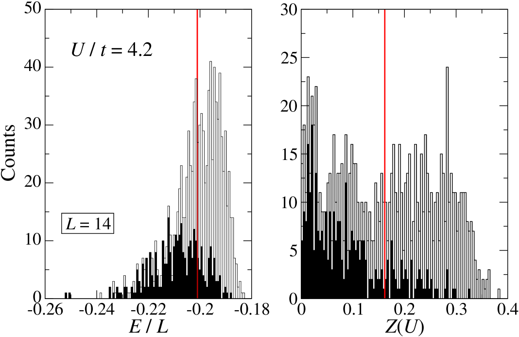
Figure 11: Histograms of the ground-state energy (left) and the quasi-particle weight (right) for $U/t=4.2$ and $L=14$ sites. Filled bars: configurations with double occupancy $d_{\cal Q}<0.053$ in Fig. 5; unfilled bars: configurations with double occupancy $d_{\cal Q}>0.053$ in Fig. 5.

In order to test this hypothesis, we present the histograms for the quasi-particle weight and the ground-state energy for $U/t=4.2$ and $L=14$ in Fig. 11. In the figure, we distinguish between ‘metallic’ configurations with $d_{\cal Q}(U/t=4.2)>0.053$ and ‘insulating’ configurations with $d_{\cal Q}(U/t=4.2)<0.053$. As can be seen, indeed, configurations with a small value of $d_{\cal Q}(U/t=4.2)$ have a strong tendency to have a small value of $Z_{\cal Q}(U/t=4.2)$, i.e., they are rather ‘insulating’ than ‘metallic’. Correspondingly, the quasi-particle weight will go up if we disregard the ‘insulating solutions’ in the average of $Z(U;L)$ and its finite-size extrapolation.

The ‘insulating’ configurations have a lower ground-state energy than the ‘metallic’ configurations. Disregarding the ‘insulating’ configurations would increase the RDA prediction for the ground-state energy and possibly improve the agreement with the QMC data. Note, however, that the insulating solution of the DMFT equations has a higher ground-state energy than the metallic solution in the coexistence regime. Therefore, the interpretation that the disregarded configurations correspond to the insulating solution in the coexistence regime is problematic.

In order to investigate further the meaning of ‘metallic’ and ‘insulating’ configurations, bigger systems with more configurations must be analyzed. Systems with $L\leq 12$ do not show the clear double-peak structure for the double occupancy as seen for $L=14$ in Fig. 5. Therefore, we cannot provide a separate finite-size extrapolation of the data for ‘metallic’ and ‘insulating’ configurations. A ‘filter’ which distinguishes between ‘metallic’ and ‘insulating’ configurations would introduce some uncontrolled bias which would act against the construction principle on which the Random Dispersion Approximation is based.

5 Conclusions

In this work, we have used the Random Dispersion Approximation (RDA) to investigate the Hubbard model at half band filling on a Bethe lattice with infinite coordination number. We have employed the numerical exact diagonalization method in real space to calculate the ground-state energy, the average double occupancy, the momentum distribution, and the quasi-particle weight for 1000 realizations of the dispersion relation on systems with $6\leq L\leq 14$ lattice sites for various interaction strengths. We reproduce earlier RDA results with a higher resolution because we have used twenty times more configurations than in previous investigations RDA ; EvaFlorian ; SandraFlorian .

In principle, the RDA describes the Hubbard model in infinite dimensions adequately, but its usefulness is limited by the small system sizes which can be treated using the Lanczos technique. The quantitative agreement with results for physical quantities in the weak-coupling and strong-coupling limits of the Hubbard model in infinite dimensions is satisfactory, but finite-size effects clearly reduce the significance of its prediction of a continuous Mott-Hubbard metal-to-insulator transition at $U_{\rm c}\approx W$ ($W$: bandwidth).

Numerical treatments of the Dynamical Mean-Field Theory for the Hubbard model in infinite dimensions indicate that the Mott-Hubbard transition is discontinuous with a finite coexistence region $U_{{\rm c},1}<U<U_{{\rm c},2}$ for a metallic and an insulating solution. In the present study, we find that the histograms, e.g., for the double occupancy, are actually bimodal in some energy interval $W<U<1.5W$, which could be interpreted as the signature of a coexistence region of ‘insulating’ and ‘metallic’ random configurations. In the thermodynamic limit, one of the two peaks should shrink to zero and reveal the unique metallic or insulating ground state. In order to corroborate this hypothesis, much larger system sizes must be analyzed.

The RDA to the Hubbard model is free of the problems that are generated by the mapping of the Hubbard model in infinite dimensions to a single-impurity problem whose properties must be determined self-consistently. If the RDA calculations could be done on larger system sizes, the concept of a discontinuous Mott-Hubbard transition could be verified independently.

References

- (1) N.F. Mott, Metal–Insulator Transitions, 2nd edition (Taylor and Francis, London, 1990).
- (2) F. Gebhard, The Mott Metal–Insulator Transition (Springer, Berlin, 1997).
- (3) S. Sachdev, Quantum Phase Transitions (Cambridge University Press, 1999).
- (4) F.H.L. Essler, H. Frahm, F. Göhmann, A. Klümper, and V.E. Korepin, The One-Dimensional Hubbard Model (Cambridge University Press, 2005).
- (5) F. Gebhard and A.E. Ruckenstein, Phys. Rev. Lett. 68, (1992), 244.
- (6) W. Metzner and D. Vollhardt, Phys. Rev. Lett. 62, (1989) 324.
- (7) E. Müller-Hartmann, Z. Phys. B 74, (1989) 507.
- (8) M. Jarrell, Phys. Rev. Lett. 69, (1992) 168.
- (9) A. Georges, G. Kotliar, W. Krauth, and M.J. Rozenberg, Rev. Mod. Phys. 68, (1996) 13.
- (10) R.M. Noack and F. Gebhard, Phys. Rev. Lett. 82, (1999) 1915.
- (11) J. Hubbard, Proc. Roy. Soc. London Ser. A 276, (1963) 238; ibid. 277, (1963) 237.
- (12) P.G.J. van Dongen, F. Gebhard, and D. Vollhardt, Z. Phys. B 76, (1989) 199.
- (13) E. Economou, Green’s Functions in Quantum Physics, 2nd edition (Springer, Berlin, 1983).
- (14) S. Nishimoto, E. Jeckelmann, F. Gebhard, and R.M. Noack, Phys. Rev. B 65, 165114 (2002).
- (15) D. Ruhl and F. Gebhard, J. Stat. Mech. Exp. Theor. (2006) P03015.
- (16) M.P. Eastwood, F. Gebhard, E. Kalinowski, S. Nishimoto, and R.M. Noack, Eur. Phys. J. B 35, (2003) 155.
- (17) N. Blümer and E. Kalinowski, Phys. Rev. B 71, (2005) 195102; Physica B 359-361, (2005) 648.
- (18) S. Nishimoto, F. Gebhard, and E. Jeckelmann, J. Phys. Cond. Matt. 16, (2004) 7063.
- (19) S. Nishimoto, private communication (2007).
- (20) N. Blümer, private communication (2008).
- (21) F. Gebhard, E. Jeckelmann, S. Mahlert, S. Nishimoto, and R.M. Noack, Eur. Phys. J. B 36, (2003) 491.
- (22) R. Bulla, Phys. Rev. Lett. 83, 136 (1999); R. Bulla, private communication (2002).
- (23) S. Nishimoto, F. Gebhard, and E. Jeckelmann, Physica B 378, (2006) 283.
- (24) M. Karski, C. Raas, and G.S. Uhrig, Phys. Rev. B 72, (2005) 113110; ibid. 77, (2008) 075116.
- (25) G. Kotliar and D. Vollhardt, Physics Today 57, No. 3 (2004) 53.
- (26) P. Majumdar and H.R. Krishnamurti, Phys. Rev. Lett. 73, (1994) 1525; Phys. Rev. B. 52, (1995) 5479.
- (27) S. Kehrein, Phys. Rev. Lett. 81, (1998) 3912; A. Georges and G. Kotliar, ibid. 84, (2000) 3500; S. Kehrein, ibid. 84, (2000) 3501.
- (28) W. Metzner, Phys. Rev. B 43, (1991) 8549.
- (29) D.E. Logan and P. Nozières, Phil. Trans. Roy. Soc. A356, (1998) 249; P. Nozières, Eur. Phys. J. B 6, (1998) 447.