Recent developments in superstatistics

Abstract

We provide an overview on superstatistical techniques applied to complex systems with time scale separation. Three examples of recent applications are dealt with in somewhat more detail: the statistics of small-scale velocity differences in Lagrangian turbulence experiments, train delay statistics on the British rail network, and survival statistics of cancer patients once diagnosed with cancer. These examples correspond to three different universality classes: Lognormal superstatistics, $\chi^{2}$-superstatistics and inverse $\chi^{2}$ superstatistics.

I Introduction

Many complex systems in various areas of science exhibit a spatio-temporal dynamics that is inhomogeneous and can be effectively described by a superposition of several statistics on different scales, in short a ’superstatistics’ beck-cohen ; unicla ; touchette ; supergen ; souza ; chavanis ; vignat ; Plastino-x ; jizba ; wilk ; prl01 . The superstatistics notion was introduced in beck-cohen , in the mean time many applications for a variety of complex systems have been pointed out daniels ; maya ; reynolds ; RMT ; abul-magd3 ; porpo ; rapisarda ; kantz ; cosmic ; eco ; straetennew ; eco2 . Essential for this approach is the existence of sufficient time scale separation between two relevant dynamics within the complex system. There is an intensive parameter $\beta$ that fluctuates on a much larger time scale than the typical relaxation time of the local dynamics. In a thermodynamic setting, $\beta$ can be interpreted as a local inverse temperature of the system, but much broader interpretations are possible.

The stationary distributions of superstatistical systems, obtained by averaging over all $\beta$, typically exhibit non-Gaussian behavior with fat tails, which can be a power law, or a stretched exponential, or other functional forms as well touchette . In general, the superstatistical parameter $\beta$ need not to be an inverse temperature but can be an effective parameter in a stochastic differential equation, a volatility in finance, or just a local variance parameter extracted from some experimental time series. Many applications have been recently reported, for example in hydrodynamic turbulence prl ; beck03 ; reynolds ; unicla , for defect turbulence daniels , for cosmic rays cosmic and other scattering processes in high energy physics wilknew ; superscatter , solar flares maya , share price fluctuations bouchard ; ausloos ; eco ; straetennew , random matrix theory RMT ; abul-magd2 ; abul-magd3 , random networks abe-thurner , multiplicative-noise stochastic processes queiros , wind velocity fluctuations rapisarda ; kantz , hydro-climatic fluctuations porpo , the statistics of train departure delays briggs and models of the metastatic cascade in cancerous systems chen . On the theoretical side, there have been recent efforts to formulate maximum entropy principles for superstatistical systems souza ; abc ; crooks ; naudts ; straeten .

In this paper we provide an overview over some recent developments in the area of superstatistics. Three examples of recent applications are discussed in somewhat more detail: the statistics of Lagrangian turbulence, the statistics of train departure delays, and the survival statistics of cancer patients. In all cases the superstatistical model predictions are in very good agreement with real data. We also comment on recent theoretical approaches to develop generalized maximum entropy principles for superstatistical systems.

II Motivation for superstatistics

In generalized versions of statistical mechanics one starts from more general entropic measures than the Boltzmann-Gibbs Shannon entropy. A well-known example is the $q$-entropy tsallis ; mendes

$$S_{q}=\frac{1}{q-1}(\sum_{i}p_{i}^{q}-1)$$

but other forms are possible as well (see, e.g., gentropy for a recent review). The $p_{i}$ are the probabilities of the microstates $i$, and $q$ is a real number, the entropic index. The ordinary Shannon entropy is contained as the special case $q=1$:

$$\lim_{q\to 1}S_{q}=S_{1}=-\sum_{i}p_{i}\log p_{i}$$

Extremizing $S_{q}$ subject to suitable constraints yields more general canonical ensembles, where the probability to observe a microstate with energy $E_{i}$ is given by

$$p_{i}\sim e_{q}^{-\beta E_{i}}:=\frac{1}{(1+(q-1)\beta E_{i})^{\frac{1}{q-1}}}$$

One obtains a kind of power-law Boltzmann factor, of the so-called $q$-exponential form. The important question is what could be a physical (non-equilibrium mechanism) to obtain such distributions.

The reason could indeed be a driven nonequilibrium situation with local fluctuations of the environment. This is the situation where the superstatistics concept enters. Our starting point is the following well-known formula

$$\int_{0}^{\infty}d\beta f(\beta)e^{-\beta E}=\frac{1}{(1+(q-1)\beta_{0}E)^{1/(q-1)}}$$

where

$$f(\beta)=\frac{1}{\Gamma\left(\frac{1}{q-1}\right)}\left\{\frac{1}{(q-1)\beta_{0}}\right\}^{\frac{1}{q-1}}\beta^{\frac{1}{q-1}-1}\exp\left\{-\frac{\beta}{(q-1)\beta_{0}}\right\}$$

is the $\chi^{2}$ (or $\Gamma$) probability distribution.

We see that averaged ordinary Boltzmann factors with $\chi^{2}$ distributed $\beta$ yield a generalized Boltzmann factor of $q$-exponential form. The physical interpretation is that Tsallis’ type of statistical mechanics is relevant for nonequilibrium systems with temperature fluctuations. This approach was made popular by two PRLs in 2000/2001 wilk ; prl01 , which used the $\chi^{2}$-distribution for $f(\beta)$. General $f(\beta)$ were then discussed in beck-cohen .

In prl01 it was suggested to construct a dynamical realization of $q$-statistics in terms of e.g. a linear Langevin equation

$$\dot{v}=-\gamma v+\sigma L(t)$$

with fluctuating parameters $\gamma,\sigma$. Here $L(t)$ denotes Gaussian white noise. The parameters $\gamma,\sigma$ are supposed to fluctuate on a much larger time scale than the ’velocity’ $v$. One can think of a Brownian particle that moves through spatial ’cells’ with different local $\beta:=\gamma/(2\sigma^{2})$ in each cell (a nonequilibrium situation). Assume the probability distribution of $\beta$ in the various cells is a $\chi^{2}$-distribution of degree $n$:

$$f(\beta)\sim\beta^{n/2-1}e^{-\frac{n\beta}{2\beta_{0}}}$$

Then the conditional probability given some fixed $\beta$ in a given cell is Gaussian, $p(v|\beta))\sim e^{-\frac{1}{2}\beta v^{2}}$, the joint probability is $p(v,\beta)=f(\beta)p(v|\beta)$ and the marginal probability is $p(v)=\int_{0}^{\infty}f(\beta)p(v|\beta)d\beta$. Integration yields

$$p(v)\sim\frac{1}{(1+\frac{1}{2}\tilde{\beta}(q-1)v^{2})^{1/(q-1)}},$$

i.e. we obtain power-law Boltzmann factors with $q=1+\frac{2}{n+1}$, $\tilde{\beta}=2\beta_{0}/(3-q)$, and $E=\frac{1}{2}v^{2}$. Here $\beta_{0}=\int f(\beta)\beta d\beta$ is the average of $\beta$.

The idea of superstatistics is to generalize this example to much broader systems. For example, $\beta$ need not be an inverse temperature but can in principle be any intensive parameter. Most importantly, one can generalize to general probability densities $f(\beta)$ and general Hamiltonians. In all cases one obtains a superposition of two different statistics: that of $\beta$ and that of ordinary statistical mechanics. Superstatistics hence describes complex nonequilibrium systems with spatio-temporal fluctuations of an intensive parameter on a large scale. The effective Boltzmann factors $B(E)$ for such systems are given by

$$B(E)=\int_{0}^{\infty}f(\beta)e^{-\beta E}d\beta.$$

Some recent theoretical developments of the superstatistics concept include the following:

• Can prove a superstatistical generalization of fluctuation theorems supergen

• Can develop a variational principle for the large-energy asymptotics of general superstatistics touchette (depending on $f(\beta)$, one can get not only power laws for large $E$ but e.g. also stretched exponentials)

• Can formally define generalized entropies for general superstatistics souza ; abc ; straeten

• Can study microcanonical superstatistics (related to a mixture of $q$-values) vignat

• Can prove a superstatistical version of a Central Limit Theorem leading to $q$-statistics Plastino-x

• Can relate it to fractional reaction equations hau

• Can consider superstatistical random matrix theory RMT ; abul-magd2 ; abul-magd3

• Can apply superstatistical techniques to networks abe-thurner

• Can define superstatistical path integrals jizba

• Can do superstatistical time series analysis unicla ; kantz ; straetennew

…and some more practical applications:

• Can apply superstatistical methods to analyze the statistics of 3d hydrodynamic turbulence beck03 ; reynolds ; unicla ; prl

• Can apply it to atmospheric turbulence (wind velocity fluctuations rapisarda ; kantz )

• Can apply superstatistical methods to finance and economics ausloos ; eco2 ; heston ; bouchard

• Can apply it to blinking quantum dots grigolini

• Can apply it to cosmic ray statistics cosmic

• Can apply it to various scattering processes in particle physics wilknew ; superscatter

• Can apply it to hydroclimatic fluctuations porpo

• Can apply it to train delay statistics briggs

• Can consider medical applications chen

III Observed universality classes

While in principle any $f(\beta)$ is possible in the superstatistics approach, in practice one usually observes only a few relevant distributions. These are the $\chi^{2}$, inverse $\chi^{2}$ and lognormal distribution. In other words, in typical complex systems with time scale separation one usually observes 3 physically relevant universality classes unicla

• (a) $\chi^{2}$-superstatistics ($=$ Tsallis statistics)

• (b) inverse $\chi^{2}$-superstatistics

• (c) lognormal superstatistics

What could be a plausible reason for this? Consider, e.g., case (a). Assume there are many microscopic random variables $\xi_{j}$, $j=1,\ldots,J$, contributing to $\beta$ in an additive way. For large $J$, the sum $\frac{1}{\sqrt{J}}\sum_{j=1}^{J}\xi_{j}$ will approach a Gaussian random variable $X_{1}$ due to the (ordinary) Central Limit Theorem. There can be $n$ Gaussian random variables $X_{1},\ldots,X_{n}$ of the same variance due to various relevant degrees of freedom in the system. $\beta$ should be positive, hence the simplest way to get such a positive $\beta$ is to square the Gaussian random variables and sum them up. As a result, $\beta=\sum_{i=1}^{n}X_{i}^{2}$ is $\chi^{2}$-distributed with degree $n$,

$$f(\beta)=\frac{1}{\Gamma(\frac{n}{2})}\left(\frac{n}{2\beta_{0}}\right)^{n/2}\beta^{n/2-1}e^{-\frac{n\beta}{2\beta_{0}}},$$ (1)

where $\beta_{0}$ is the average of $\beta$.

(b) The same considerations can be applied if the ’temperature’ $\beta^{-1}$ rather than $\beta$ itself is the sum of several squared Gaussian random variables arising out of many microscopic degrees of freedom $\xi_{j}$. The resulting $f(\beta)$ is the inverse $\chi^{2}$-distribution:

$$f(\beta)=\frac{\beta_{0}}{\Gamma(\frac{n}{2})}\left(\frac{n\beta_{0}}{2}\right)^{n/2}\beta^{-n/2-2}e^{-\frac{n\beta_{0}}{2\beta}}.$$ (2)

It generates superstatistical distributions $p(E)\sim\int f(\beta)e^{-\beta E}$ that decay as $e^{-\tilde{\beta}\sqrt{E}}$ for large $E$.

(c) $\beta$ may be generated by multiplicative random processes. Consider a local cascade random variable $X_{1}=\prod_{j=1}^{J}\xi_{j}$, where $J$ is the number of cascade steps and the $\xi_{j}$ are positive microscopic random variables. By the (ordinary) Central Limit Theorem, for large $J$ the random variable $\frac{1}{\sqrt{J}}\log X_{1}=\frac{1}{\sqrt{J}}\sum_{j=1}^{J}\log\xi_{j}$ becomes Gaussian for large $J$. Hence $X_{1}$ is log-normally distributed. In general there may be $n$ such product contributions to $\beta$, i.e., $\beta=\prod_{i=1}^{n}X_{i}$. Then $\log\beta=\sum_{i=1}^{n}\log X_{i}$ is a sum of Gaussian random variables, hence it is Gaussian as well. Thus $\beta$ is log-normally distributed, i.e.,

$$f(\beta)=\frac{1}{\sqrt{2\pi}s\beta}\exp\left\{\frac{-(\ln\frac{\beta}{\mu})^{2}}{2s^{2}}\right\},$$ (3)

where $\mu$ and $s$ are suitable parameters.

IV Application to traffic delays

We will now discuss examples of the three different superstatistical universality classes. Our first example is the departure delay statistics on the British rail network. Clearly, at the various stations there are sometimes train departure delays of length $t$. The 0th-order model for the waiting time would be a Poisson process which predicts that the waiting time distribution until the train finally departs is $P(t|\beta)=\beta e^{-\beta t}$, where $\beta$ is some parameter. But this does not agree with the actually observed data briggs . A much better fit is given by a $q$-exponential, see Fig. 1.

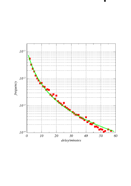
Figure 1: Observed departure delay statistics on the British railway network (data from briggs ). The solid line is a q-exponential fit as given by eq. (5).

What may cause this power law that fits the data? The idea is that there are fluctuations in the parameter $\beta$ as well. These fluctuations describe large-scale temporal or spatial variations of the British rail network environment. Examples of causes of these $\beta$-fluctuations:

• begin of the holiday season with lots of passengers

• problem with the track

• bad weather conditions

• extreme events such as derailments, industrial action, terror alerts, etc.

As a result, the long-term distribution of train delays is then a mixture of exponential distributions where the parameter $\beta$ fluctuates:

$$p(t)=\int_{0}^{\infty}f(\beta)p(t|\beta)d\beta=\int_{0}^{\infty}f(\beta)\beta e^{-\beta t}.$$ (4)

For a $\chi^{2}$-distributed $\beta$ with $n$ degrees of freedom one obtains

$$p(t)\sim{\left(1+b(q-1)t\right)^{\frac{1}{1-q}}}$$ (5)

where $q=1+{2}/(n+2)$ and $b={2}\beta_{0}/({2-q})$. The model discussed in briggs generates $q$-exponential distributions of train delays by a simple mechanism, namely a $\chi^{2}$-distributed parameter $\beta$ of the local Poisson process. This is an example for $\chi^{2}$ superstatistics.

V Application to turbulence

Our next example is an application in turbulence. Consider a single tracer particle advected by a fully developed turbulent flow. For a while it will see regions of strong turbulent activity, then move on to calmer regions, just to continue in yet another region of strong activity, and so on. This is a superstatistical dynamics, and in fact superstatistical models of turbulence have been very successful in recent years reynolds ; prl . The typical shape of a trajectory of such a tracer particle is plotted in Fig. 2.

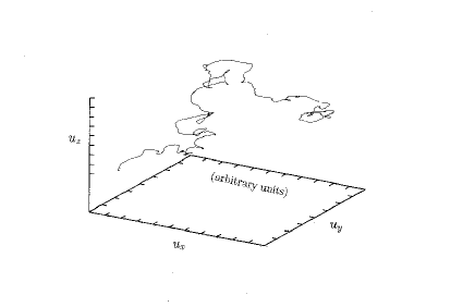
Figure 2: Typical example of a trajectory of a test particle in a turbulent flow.

This is ’Lagrangian turbulence’ in contrast to ’Eulerian turbulence’, meaning that one is following a single particle in the flow. In particular, one is interested in velocity differences $\vec{u}(t):=\vec{v}(t+\tau)-\vec{v}(t)$ of the particle on a small time scale $\tau$. For $\tau\to 0$ this velocity difference becomes the local acceleration $\vec{a}(t)=\vec{u}(t)/\tau$. A superstatistical Lagrangian model for 3-dim velocity differences of the tracer particle has been developed in prl . One simply looks at a superstatistical Langevin equation of the form

$$\dot{\vec{u}}=-\gamma\vec{u}+B\vec{n}\times\vec{u}+\sigma\vec{L}(t).$$ (6)

Here $\gamma$ and $B$ are constants. Note that the term proportional to $B$ introduces some rotational movement of the particle, mimicking the vortices in the flow. The noise strength $\sigma$ and the unit vector $\vec{n}$ evolve stochastically on a large time scale $T_{\sigma}$ and $T_{\vec{n}}$, respectively, thus obtaining a superstatistical dynamics. $T_{\sigma}$ is of the same order of magnitude as the integral time scale $T_{L}$, whereas $\gamma^{-1}$ is of the same order of magnitude as the Kolmogorov time scale $\tau_{\eta}$. One can show that the Reynolds number $R_{\lambda}$ is basically given by the time scale ratio $T_{\sigma}\gamma\sim T_{L}/\tau_{\eta}\sim R_{\lambda}>>1$. The time scale $T_{\vec{n}}>>\tau_{\eta}$ describes the average life time of a region of given vorticity surrounding the test particle.

In this superstatistical turbulence model one defines the parameter $\beta$ to be $\beta:=2\gamma/\sigma^{2}$, but it does not have the meaning of a physical inverse temperature in the flow. Rather, one has $\beta^{-1}\sim\nu^{1/2}\langle\epsilon\rangle^{-1/2}\epsilon$, where $\nu$ is the kinematic viscosity and $\langle\epsilon\rangle$ is the average energy dissipation, which is known to fluctuate in turbulent flows. In fact, Kolmogorov’s theory of 1961 suggests a lognormal distribution for $\epsilon$, which automatically leads us to lognormal superstatistics: It is reasonable to assume that the probability density of the stochastic process $\beta(t)$ is approximately a lognormal distribution

$$f(\beta)=\frac{1}{\beta s\sqrt{2\pi}}\exp\left\{\frac{-(\log\frac{\beta}{m})^{2}}{2s^{2}}\right\}.$$ (7)

For very small $\tau$ the 1d acceleration component of the particle is given by $a_{x}=u_{x}/\tau$ and one gets out of the model the 1-point distribution

$$p(a_{x})=\frac{\tau}{2\pi s}\int_{0}^{\infty}d\beta\;\beta^{-1/2}\exp\left\{\frac{-(\log\frac{\beta}{m})^{2}}{2s^{2}}\right\}e^{-\frac{1}{2}\beta\tau^{2}a_{x}^{2}}.$$ (8)

This prediction agrees very well with experimentally measured data of the acceleration statistics, which exhibits very pronounced (non-Gaussian) tails, see Fig. 3 for an example.

Figure 3: Measured probability density of small-scale velocity differences in Lagrangian turbulence (data from pinton ). The solid line is a fit of the form (8) (see prl for more details).

It is interesting to see that our 3-dimensional superstatistical model predicts the existence of correlations between the acceleration components. For example, the acceleration $a_{x}$ in $x$ direction is not statistically independent of the acceleration $a_{y}$ in $y$-direction. We may study the ratio $R:=p(a_{x},a_{y})/(p(a_{x})p(a_{y}))$ of the joint probability $p(a_{x},a_{y})$ to the 1-point probabilities $p(a_{x})$ and $p(a_{y})$. For independent acceleration components this ratio would always be given by $R=1$. However, our 3-dimensional superstatistical model yields prediction

$$R=\frac{\int_{0}^{\infty}\beta f(\beta)e^{-\frac{1}{2}\beta\tau^{2}(a_{x}^{2}+a_{y}^{2})}d\beta}{\int_{0}^{\infty}\beta^{1/2}f(\beta)e^{-\frac{1}{2}\beta\tau^{2}a_{x}^{2}}d\beta\int_{0}^{\infty}\beta^{1/2}f(\beta)e^{-\frac{1}{2}\beta\tau^{2}a_{y}^{2}}d\beta}$$ (9)

This is a very general formula, valid for any superstatistics, for example also Tsallis statistics, obtained when $f(\beta)$ is the $\chi^{2}$-distribution. The trivial result $R=1$ is obtained only for $f(\beta)=\delta(\beta-\beta_{0})$, i.e. no fluctuations in the parameter $\beta$ at all. Fig. 4 shows $R:=p(a_{x},a_{y})/(p(a_{x})p(a_{y}))$ as predicted by lognormal superstatistics:

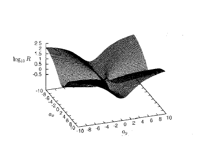
Figure 4: Predicted shape of correlations as given by eq. (9), $f(\beta)$ being the lognormal distribution.

The shape of this is very similar to experimental measurements boden-reynolds ; prl .

VI Application in medicine

Our final example of application of superstatistics is for a completely different area: medicine. We will look at cell migration processes describing the metastatic cascade of cancerous cells in the body chen . There are various pathways in which cancerous cells can migrate: Via the blood system, the lymphatic system, and so on. The diffusion constants for these various pathways are different. In this way superstatistics enters, describing different diffusion speeds for different pathways (see Fig. 5).

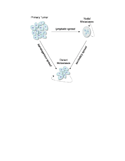
Figure 5: Various pathways for the spread of cancer cells

But there is another important issue here: When looking at a large ensemble of patients then the spread of cancerous cells can be very different from patient to patient. For some patients the cancer spreads in a very aggressive way, whereas for others it is much slower and less aggressive. So superstatistics also arises from the fact that all patients are different.

A superstatistical model of metastasis and cancer survival has been developed in chen . Details are described in that paper. Here we just mention the final result that comes out of the model: One obtains the following prediction for the probability density function of survival time $t$ of a patient that is diagnosed with cancer at $t=0$:

$$p\left(t\right)=\int_{0}^{\infty}\!{\frac{{t}^{n-1}{\lambda}^{n}{e^{-\lambda\,t}}}{\Gamma\left(n\right)}\frac{\lambda_{0}{\left(n\lambda_{0}/2\right)}^{n/2}}{\Gamma\left(n/2\right)}\lambda^{-n/2-2}e^{\frac{-n\lambda_{0}}{2\lambda}}}{d\lambda},$$ (10)

or

$$p\left(t\right) = \frac{(n\lambda_{0})^{3n/4}}{\Gamma(n)\Gamma(n/2)}\left(\frac{t}{2}\right)^{3n/4-1}\left[\frac{\sqrt{2n\lambda_{0}t}}{n}K_{n/2+1}\left(\sqrt{2n\lambda_{0}t}\right)\right.$$ (11)

$$- \left.K_{n/2}\left(\sqrt{2n\lambda_{0}t}\right)\right],$$

where $K_{\nu}(z)$ is the modified Bessel function. Note that this is inverse $\chi^{2}$ superstatistics. The role of the parameter $\beta$ is now played by the parameter $\lambda$, which in a sense describes how aggressively the cancer propagates.

The above formula based on inverse $\chi^{2}$ superstatistics is in good agreement with real data of the survival statistics of breast cancer patients in the US. The superstatistical formula fits the observed distribution very well, both in a linear and logarithmic plot (see Fig.6).

One remark is at order. When looking at the relevant time scales one should keep in mind that the data shown are survival distributions conditioned on the fact that death occurs due to cancer. Many patients, in particular if they are diagnosed at an early stage, will live a long happy life and die from something else than cancer. These cases are not included in the data.

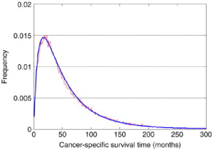
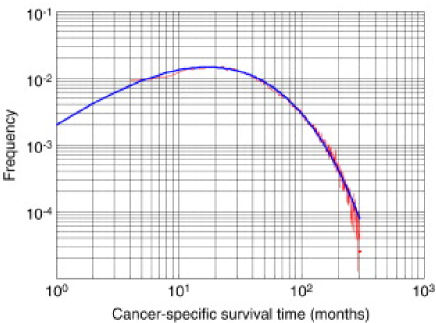
Figure 6: Survival time statistics of breast cancer patients once diagnosed with cancer $(t=0)$, both in a linear and double logarithmic plot. Only patients that die from cancer are included in the statistics. The solid line is the superstatistical model prediction chen .

VII Maximum entropy principles, superstatistical path integrals, and more

We finish this article by briefly mentioning some other recent interesting theoretical developments.

One major theoretical concern is that a priori the superstatistical distribution $f(\beta)$ can be anything. But perhaps one should single out the really relevant distributions $f(\beta)$ by a least biased guess, given some constraints on the complex system under consideration. This program has been developed in some recent papers abc ; straeten . There are some ambiguities which constraints should be implemented, and how. A very general formalism is presented in straeten , which contains previous work abc ; crooks ; naudts as special cases. The three important universality classes discussed above, namely $\chi^{2}$ superstatistics, inverse $\chi^{2}$ superstatistics and lognormal superstatistics are contained as special cases in the formalism of straeten . In principle, once a suitable generalized maximum entropy principle has been formulated for superstatistical systems, one can proceed to a generalized thermodynamic description, get a generalized equation of state, and so on. There is still a lot of scope of future research to develop the most suitable formalism. But the general tendency seems to be to apply maximum entropy principles and least biased guesses to nonequilibrium situations as well. In fact, Jaynes jaynes always thought this is possible.

Another interesting development is what one could call a superstatistical path integral. These are just ordinary path integrals but with an additional integration over a parameter $\beta$ that make the Wiener process become something more complicated, due to large-scale fluctuations of its diffusion constant. Jizba et al. investigate under which conditions one obtains a Markov process again jizba . It seems some distributions $f(\beta)$ are distinguished as making the superstatistical process simpler than others, preserving Markovian-like properties. These types of superstatistical path integral processes have applications in finance, and possibly also in quantum field theory and elementary particle physics.

In high energy physics, many of the power laws observed for differential cross sections and energy spectra in high energy scattering processes can also be explained using superstatistical models wilknew ; superscatter . The key point here is to extend the Hagedorn theory hage to a superstatistical one which properly takes into account temperature fluctuations beck00 ; superscatter . Superstatistical techniques have also been recently used to describe the space-time foam in string theory kings .

VIII Summary

Superstatistics (a ’statistics of a statistics’) provides a physical reason why more general types of Boltzmann factors ( e.g. $q$-exponentials or other functional forms) are relevant for nonequilibrium systems with suitable fluctuations of an intensive parameter. Let us summarize:

• There is evidence for three major physically relevant universality classes: $\chi^{2}$-superstatistics $=$ Tsallis statistics, inverse $\chi^{2}$-superstatistics, and lognormal superstatistics. These arise as universal limit statistics for many different systems.

• Superstatistical techniques can be successfully applied to a variety of complex systems with time scale separation.

• The train delays on the British railway network are an example of $\chi^{2}$ superstatistics = Tsallis statistics briggs .

• A superstatistical model of Lagrangian turbulence prl is in excellent agreement with the experimental data for probability densities, correlations between components, decay of correlations, Lagrangian scaling exponents, etc. This is an example of lognormal superstatistics prl .

• Cancer survival statistics is described by inverse $\chi^{2}$ superstatistics chen .

• The long-term aim is to find a good thermodynamic description for general superstatistical systems. A generalized maximum entropy principle may help to achieve this goal.

References

- (1) C. Beck and E.G.D. Cohen, Physica A 322, 267 (2003)
- (2) C. Beck, E.G.D. Cohen, and H.L. Swinney, Phys. Rev. E 72, 056133 (2005)
- (3) C. Beck and E.G.D. Cohen, Physica A 344, 393 (2004)
- (4) H. Touchette and C. Beck, Phys. Rev. E 71, 016131 (2005)
- (5) C. Tsallis and A.M.C. Souza, Phys. Rev. E 67, 026106 (2003)
- (6) P. Jizba, H. Kleinert, Phys. Rev. E 78, 031122 (2008)
- (7) C. Vignat, A. Plastino and A.R. Plastino, cond-mat/0505580
- (8) C. Vignat, A. Plastino, arXiv 0706.0151
- (9) P.-H. Chavanis, Physica A 359, 177 (2006)
- (10) G. Wilk and Z. Wlodarczyk, Phys. Rev. Lett. 84, 2770 (2000)
- (11) C. Beck, Phys. Rev. Lett. 87, 180601 (2001)
- (12) K. E. Daniels, C. Beck, and E. Bodenschatz, Physica D 193, 208 (2004)
- (13) C. Beck, Physica A 331, 173 (2004)
- (14) M. Baiesi, M. Paczuski and A.L. Stella, Phys. Rev. Lett. 96, 051103 (2006)
- (15) Y. Ohtaki and H.H. Hasegawa, cond-mat/0312568
- (16) A.Y. Abul-Magd, Physica A 361, 41 (2006)
- (17) S. Rizzo and A. Rapisarda, AIP Conf. Proc. 742, 176 (2004) (cond-mat/0406684)
- (18) T. Laubrich, F. Ghasemi, J. Peinke, H. Kantz, arXiv:0811.3337
- (19) A. Porporato, G. Vico, and P.A. Fay, Geophys. Res. Lett. 33, L15402 (2006)
- (20) A. Reynolds, Phys. Rev. Lett. 91, 084503 (2003)
- (21) H. Aoyama et al., arXiv:0805.2792
- (22) E. Van der Straeten, C. Beck, arXiv:0901.2271
- (23) A.Y. Abul-Magd, G. Akemann, P. Vivo, arXiv 0811.1992
- (24) C. Beck, Europhys. Lett. 64, 151 (2003)
- (25) C. Beck, Phys. Rev. Lett. 98, 064502 (2007)
- (26) G. Wilk, Z. Wlodarczyk, arXiv:0810.2939
- (27) C. Beck, arXiv:0902.2459
- (28) M. Ausloos and K. Ivanova, Phys. Rev. E 68, 046122 (2003)
- (29) J.-P. Bouchard and M. Potters, Theory of Financial Risk and Derivative Pricing, Cambridge University Press, Cambridge (2003)
- (30) A.Y. Abul-Magd, B. Dietz, T. Friedrich, A. Richer, Phys. Rev. E 77, 046202 (2008)
- (31) S. Abe and S. Thurner, Phys. Rev. E 72, 036102 (2005)
- (32) Sílvio M. Duarte Queirós, Braz. J. Phys. 38, 203 (2008)
- (33) K. Briggs, C. Beck, Physica A 378, 498 (2007)
- (34) L. Leon Chen, C. Beck, Physica A 387, 3162 (2008)
- (35) S. Abe, C. Beck and G. D. Cohen, Phys. Rev. E 76, 031102 (2007)
- (36) G. E. Crooks, Phys. Rev. E 75, 041119 (2007)
- (37) J. Naudts, AIP Conference Proceedings 965, 84 (2007)
- (38) E. Van der Straeten, C. Beck, Phys. Rev. E 78, 051101 (2008)
- (39) C. Tsallis, J. Stat. Phys. 52, 479 (1988)
- (40) C. Tsallis, R.S. Mendes, A.R. Plastino, Physica A 261, 534 (1998)
- (41) C. Beck, arXiv:0902:1235, to appear in Contemporary Physics (2009)
- (42) A.M. Mathai and H.J. Haubold, Physica A 375, 110 (2007)
- (43) S.L. Heston, Rev. Fin. Studies 6, 327 (1993)
- (44) S. Bianco, P. Grigolini, P. Paradisi, cond-mat/0509608
- (45) N. Mordant, P. Metz, O. Michel, and J.-F. Pinton, Phys. Rev. Lett 87, 214501 (2001)
- (46) A.M. Reynolds, N. Mordant, A.M. Crawford, and E. Bodenschatz, New Journal of Physics 7, 58 (2005)
- (47) R. D. Rosenkrantz, E.T. Jaynes: papers on probability, statistics and statistical physics, Kluwer (1989)
- (48) R. Hagedorn, Suppl. Nuovo Cim. 3, 147 (1965)
- (49) C. Beck, Physica A 286, 164 (2000)
- (50) N.E. Mavromatos and S. Sarkar, arXiv:0812.3952