Electromagnetic waves in uniaxial crystals: General formalism with an application to Bessel beams

Abstract

We present a mathematical formalism describing the propagation of a completely general electromagnetic wave in a birefringent medium. Analytic formulas for the refraction and reflection from a plane interface are obtained. As a particular example, a Bessel beam impinging at an arbitrary angle is analyzed in detail. Some numerical results showing the formation and destruction of optical vortices are presented.

I Introduction

The phenomena of birefringence was already well known at the time when Huygens studied the “strange properties of the Island crystal” huygens with a view to proving the wave nature of light. Newton also discussed these same properties at length in his Opticks newton , but to prove precisely the contrary. In any case, a full mathematical description of the phenomena turned out to be quite cumbersome and it is only in the last few decades that analytic expressions were obtained for the simplest case of a plane electromagnetic wave in an uniaxial crystal lekner . Generalizations to more realistic waves, such as Hermite-Gauss, Laguerre-Gauss or Bessel beams, have been so far restricted to paraxial (or almost paraxial) approximations fleck ; martinez ; cia-cin-palma , and to propagations parallel cia-cin-palma2 or perpendicular cia-palma to the crystal axis.

The aim of the present work is to obtain the most general expressions describing reflected and refracted (ordinary and extraordinary) waves in terms of the properties of a beam impinging at the plane interface of a uniaxial crystal. Analytic formulas are presented in as compact a form as possible. As an example of application, the propagation of a Bessel beam durnin ; eberly is studied; these are electromagnetic modes that propagate in vacuum with an invariant intensity pattern and exhibit polarization and phase optical vortices nye yielding an electromagnetic orbital angular momentum (see, e. g., Ref. rozas ). However, as we will show in the following, the intensity pattern inside a birefringent crystal does not remain constant along the main axis of propagation (unless it coincides with the crystal symmetry axis); moreover optical vortices can be created or destroyed. Flossmann et al. flossmann ; flossmann2 considered the case of a Laguerre-Gauss beam propagating inside a birefringent crystal and analyzed the evolution of the polarization vortices in terms of Stokes parameters. Here, we apply such a study to Bessel beams using our analytical expressions, and complement it with a study of the corresponding topological features of phase diagrams.

Modern experiments of parametric down-conversion use crystals that are birefringent besides being nonlinear. These properties are particularly important for generating entangled photons with different dynamical properties determined by their source beam. Thus, for example, when a Laguerre-Gauss or a Bessel beam is taken as a pump, the down-converted light is expected to consist of entangled photons with orbital angular momentum PDC . However, the anisotropy of the birefringent crystals used for that purpose prevent a direct identification of the expected characteristics of the ordinary and extraordinary beams and, consequently, of the properties of the idler and signal photons. Although these are effects of quantum nonlinear optics, their precise characterization must be preceded by a detailed description of the classical linear effects as we present in the following.

The organization of this article is as follows. In Section 2, a formalism describing electromagnetic waves of any form inside and outside a birefringent crystal is presented; the boundary conditions at a plane interface are applied in order to obtain explicit expressions for the reflected and refracted waves. The resulting equations are used in the Section 3 to describe a Bessel beam incident at an arbitrary angle on the crystal interface (though the formalism is completely general, the optical axis is taken perpendicular to the interface for simplicity); we show that the reflected and refracted beams are given in terms of a single circuit integral. Lastly, we discuss numerical results for some specific parameters of the incident beam, following in particular the evolution of optical vortices, both for polarization and for phase.

II Propagation in a birefringent medium.

Consider an anisotropic medium described by a dielectric tensor $\epsilon_{ij}$ or, alternatively, a dyad $\widehat{\epsilon}$ such that the electric displacement is ${\bf D}=\widehat{\epsilon}\cdot{\bf E}$ and ${\bf B}=\mu{\bf H}$. For a birefringent medium,

$$\widehat{\epsilon}=\epsilon{\bf 1}+\Delta\epsilon~{}{\bf s}~{}{\bf s},$$

where ${\bf s}$ is the axis of symmetry of the medium, $\Delta\epsilon=\epsilon_{\parallel}-\epsilon$, and $\epsilon$ and $\epsilon_{\parallel}$ are the permeabilities perpendicular and parallel to the symmetry axis respectively.

The Maxwell equations in the absence of free charges and currents are

$$\nabla\cdot{\bf B}=0~{}~{},\quad\quad\nabla\times{\bf E}+\frac{\partial{\bf B}}{\partial t}=0~{},$$ (1)

$$\nabla\cdot{\bf D}=0~{}~{},\quad\quad\nabla\times{\bf H}-\frac{\partial{\bf D}}{\partial t}=0~{}.$$ (2)

It is straightforward to see by direct substitution that their general solution for a birefringent medium is

$${\bf E}^{O}={\bf s}\times\nabla\dot{\Psi}^{O}~{},\quad~{}~{}~{}~{}{\bf E}^{E}=-\frac{1}{\epsilon}\nabla({\bf s}\cdot\nabla\Psi^{E})+\mu\ddot{\Psi}^{E}~{}{\bf s}$$ (3)

and

$${\bf H}^{O}=\frac{1}{\mu}\nabla({\bf s}\cdot\nabla\Psi^{O})-\epsilon\ddot{\Psi}^{O}~{}{\bf s}~{},\quad~{}~{}~{}~{}{\bf H}^{E}={\bf s}\times\nabla\dot{\Psi}^{E}~{}~{},$$ (4)

where ${\Psi}^{O}$ and ${\Psi}^{E}$ are Hertz potentials nisbet satisfying the two equations:

$$-\epsilon\mu\ddot{\Psi}^{O}+\nabla^{2}\Psi^{O}=0$$ (5)

and

$$-\epsilon_{\parallel}\epsilon\mu\ddot{\Psi}^{E}+\nabla\cdot\widehat{\epsilon}\cdot\nabla\Psi^{E}=0.$$ (6)

As it is well known, there are two fundamental modes: the ordinary wave with ${\bf s}\cdot{\bf E}^{O}=0$ and the extraordinary wave with ${\bf s}\cdot{\bf B}^{E}=0$. Clearly, ${\Psi}^{O}$ and ${\Psi}^{E}$ are associated to the ordinary and extraordinary waves respectively.

II.1 Boundary conditions

In the following, we restrict our analysis to harmonic fields of the form $\Psi(t,{\bf x})=e^{-i\omega t}\psi({\bf x})$. Let the vacuum be defined as the region $z<0$ and consider a wave that impinges from $z<0$ and propagates inside the medium, in the region $z>0$, with wave vectors ${\bf k}^{O}=(k_{x},k_{y},k_{z}^{O})$ and ${\bf k}^{E}=(k_{x},k_{y},k_{z}^{E})$, for the ordinary and extraordinary components respectively.

The general solution of Eqs. (5) and (6) for $z>0$ is

$$\psi^{(O,E)}(x,y,z)=\frac{1}{2\pi}\int~{}dk_{x}dk_{y}~{}e^{ik_{x}x+ik_{y}y+ik_{z}^{(O,E)}z}~{}\widetilde{\psi}^{(O,E)}(k_{x},k_{y})~{},$$ (7)

where $k_{z}^{(O,E)}$ in the integral must be taken as a function of $k_{x}$ and $k_{y}$, namely $k_{z}^{O}=(\epsilon\mu\omega^{2}-k_{x}^{2}-k_{y}^{2})^{1/2}$, and $k_{z}^{E}$ as the solution for $k_{z}$ of equation (12). Hereafter, the factor $e^{-i\omega t}$ is not included for simplicity. The two-dimensional Fourier transforms in the above formula are defined as

$$\widetilde{\psi}^{(O,E)}(k_{x},k_{y})=\frac{1}{2\pi}\int dx^{\prime}~{}dy^{\prime}~{}e^{-ik_{x}x^{\prime}-ik_{y}y^{\prime}}~{}\psi^{(O,E)}(x^{\prime},y^{\prime},0^{+}).$$ (8)

The (three-dimensional) Fourier transforms $\widetilde{{\bf E}}$ and $\widetilde{{\bf H}}$ of the electric and magnetic fields follow from Eqs. (3) and (4). Thus

$$\widetilde{{\bf E}}^{O}=\omega~{}{\bf s}\times{\bf k}^{O}~{}\widetilde{\psi}^{O}({\bf k}^{O}),\quad\widetilde{{\bf E}}^{E}=\Big{[}\frac{1}{\epsilon}({\bf s}\cdot{\bf k}^{E}){\bf k}^{E}~{}-\mu\omega^{2}~{}{\bf s}\Big{]}~{}\widetilde{\psi}^{E}({\bf k}^{E})~{},$$ (9)

and

$$\widetilde{{\bf H}}^{O}=\Big{[}-\frac{1}{\mu}({\bf s}\cdot{\bf k}^{O}){\bf k}^{O}~{}+\epsilon\omega^{2}~{}{\bf s}\Big{]}~{}\widetilde{\psi}^{O}({\bf k}^{O}),\quad\widetilde{{\bf H}}^{E}=\omega~{}{\bf s}\times{\bf k}^{E}~{}\widetilde{\psi}^{E}({\bf k}^{E})~{},$$ (10)

in obvious notation, with the conditions

$$\epsilon\mu\omega^{2}-({\bf k}^{O})^{2}=0,$$ (11)

$$\epsilon~{}\epsilon_{\parallel}\mu~{}\omega^{2}-{\bf k}^{E}\cdot\widehat{\epsilon}\cdot{\bf k}^{E}=0~{}.$$ (12)

II.2 Reflection and refraction

In order to study the reflection and refraction of the wave, we write the electric vector ${\bf E}$ in vacuum (that is, for $z<0$) in the form

$${\bf E}(x,y,z)=\frac{1}{2\pi}\int dk_{x}dk_{y}~{}e^{ik_{x}x+ik_{y}y}$$

$$\Big{[}e^{ik_{z}z}~{}\widetilde{{\bf E}}^{I}(k_{x},k_{y})+e^{-ik_{z}z}~{}\widetilde{{\bf E}}^{R}(k_{x},k_{y})\Big{]}~{},$$ (13)

where now

$$k_{z}=(\omega^{2}-k_{x}^{2}-k_{y}^{2})^{1/2}$$ (14)

and $\widetilde{{\bf E}}^{(I,R)}(k_{x},k_{y})$ are the two-dimensional Fourier transforms of the electric field components of the incident and reflected waves, ${\bf E}^{(I,R)}(x,y,0^{-})$ at the interface; similar equations apply to the magnetic field component.

The boundary conditions imply the continuity of $E_{x}$, $E_{y}$, $H_{x}$ and $H_{y}$ at the interface $z=0$ (the continuity conditions on $D_{z}$ and $B_{z}$ are not independent since, from the Maxwell equations, $i\omega D_{z}=\partial_{y}H_{x}-\partial_{x}H_{y}$ and $i\omega B_{z}=\partial_{x}E_{y}-\partial_{y}E_{x}$). It is convenient to express each Fourier transformed component of ${\bf B}$ and $E_{z}$ in the vacuum region in terms of only $E_{x}$ and $E_{y}$ using the Maxwell equations. For the incident field:

$$\widetilde{E}^{I}_{z} =-~{}\frac{1}{k_{z}}\Big{(}k_{x}\widetilde{E}^{I}_{x}+k_{y}\widetilde{E}^{I}_{y}\Big{)}$$ (15)

$$\widetilde{B}^{I}_{x} =-~{}\frac{1}{k_{z}\omega}\Big{[}k_{x}k_{y}\widetilde{E}^{I}_{x}+(k_{y}^{2}+k_{z}^{2})\widetilde{E}^{I}_{y}\Big{]}$$ (16)

$$\widetilde{B}^{I}_{y} =\frac{1}{k_{z}\omega}\Big{[}(k_{x}^{2}+k_{z}^{2})\widetilde{E}^{I}_{x}+k_{x}k_{y}\widetilde{E}^{I}_{y}\Big{]}$$ (17)

$$\widetilde{B}^{I}_{z} =~{}\frac{1}{\omega}\Big{(}-k_{y}\widetilde{E}^{I}_{x}+k_{x}\widetilde{E}^{I}_{y}\Big{)}.$$ (18)

These equations can be rewritten in diad notation as

$${\bf e}_{z}\times\widetilde{{\bf B}}^{I}=-k_{z}\omega~{}(\omega^{2}\widehat{1}-{\bf k}_{\bot}{\bf k}_{\bot})^{-1}~{}\widetilde{{\bf E}}^{I}_{\bot}$$ (19)

(here and in the following, ${\bf V}_{\bot}=(V_{x},V_{y})$ for any vector ${\bf V}$).

For the reflected field, it is only necessary to change the sign of $k_{z}$. Accordingly

$${\bf e}_{z}\times(\widetilde{{\bf B}}^{I}+\widetilde{{\bf B}}^{R})=-k_{z}\omega~{}(\omega^{2}\widehat{1}-{\bf k}_{\bot}{\bf k}_{\bot})^{-1}~{}(\widetilde{{\bf E}}^{I}_{\bot}-\widetilde{{\bf E}}^{R}_{\bot})~{},$$ (20)

and the boundary conditions take the form

$$\widetilde{{\bf E}}^{I}_{\bot}+\widetilde{{\bf E}}^{R}_{\bot}=\widetilde{{\bf E}}^{O}_{\bot}+\widetilde{{\bf E}}^{E}_{\bot}~{},$$ (21)

and

$$\widetilde{{\bf E}}^{I}_{\bot}-\widetilde{{\bf E}}^{R}_{\bot}=-~{}\frac{1}{k_{z}\omega}~{}(\omega^{2}\widehat{1}-{\bf k}_{\bot}{\bf k}_{\bot})~{}[{\bf e}_{z}\times(\widetilde{{\bf H}}^{O}+\widetilde{{\bf H}}^{E})]~{},$$ (22)

where $\widetilde{{\bf E}}^{O}$, $\widetilde{{\bf E}}^{E}$, $\widetilde{{\bf H}}^{O}$ and $\widetilde{{\bf H}}^{O}$ are to be taken from (9) and (10). The above equations form a set of four equations for the four unknown functions $\widetilde{E}^{R}_{x}$, $\widetilde{E}^{R}_{y}$, $\widetilde{\psi}^{O}$ and $\widetilde{\psi}^{E}$ in terms of $\widetilde{E}^{I}_{x}$ and $\widetilde{E}^{I}_{y}$. Explicitly we have

$$\widetilde{{\bf E}}^{I}_{\bot}+\widetilde{{\bf E}}^{R}_{\bot} = {\bf P}~{}\widetilde{\psi}^{O}+{\bf Q}~{}\widetilde{\psi}^{E}$$ (23)

$$\widetilde{{\bf E}}^{I}_{\bot}-\widetilde{{\bf E}}^{R}_{\bot} = {\bf R}~{}\widetilde{\psi}^{O}+{\bf S}~{}\widetilde{\psi}^{E}~{},$$

where

$${\bf P}=\omega({\bf s}\times{\bf k}^{O})_{\bot}~{},\quad{\bf Q}=\epsilon^{-1}~{}({\bf s}\cdot{\bf k}^{E})~{}{\bf k}_{\bot}~{}-\mu\omega^{2}~{}{\bf s}_{\bot}$$ (24)

and

$${\bf R}=\frac{\omega}{k_{z}}[\mu^{-1}~{}({\bf s}\cdot{\bf k}^{O})~{}{\bf e}_{z}\times{\bf k}_{\bot}~{}-\epsilon~{}\omega^{2}~{}{\bf e}_{z}\times{\bf s}+\epsilon~{}{\bf e}_{z}\cdot({\bf s}\times{\bf k}_{\bot})~{}{\bf k}_{\bot}],$$

$${\bf S}=\frac{\omega^{2}}{k_{z}}(s_{z}{\bf k}_{\bot}-k_{z}^{E}{\bf s}_{\bot})+\frac{1}{k_{z}}[~{}({\bf s}\cdot{\bf k}_{\bot})k_{z}^{E}-s_{z}{\bf k}_{\bot}^{2}]~{}{\bf k}_{\bot}~{}.$$ (25)

Therefore

$$\widetilde{\psi}^{O}=2~{}\frac{[{\bf e}_{z}\times({\bf Q}+{\bf S})]\cdot\widetilde{{\bf E}}^{I}}{({\bf Q}+{\bf S})\cdot[({\bf P}+{\bf R})\times{\bf e}_{z}]}$$ (26)

$$\widetilde{\psi}^{E}=-2~{}\frac{[{\bf e}_{z}\times({\bf P}+{\bf R})]\cdot\widetilde{{\bf E}}^{I}}{({\bf Q}+{\bf S})\cdot[({\bf P}+{\bf R})\times{\bf e}_{z}]}~{},$$ (27)

for the transmitted fields, and the full refracted electromagnetic field is given for all its components by Eqs. (9) and (10).

Also

$$\widetilde{{\bf E}}^{R}_{\bot}=\frac{1}{2}({\bf P}-{\bf R})\widetilde{\psi}^{O}+\frac{1}{2}({\bf Q}-{\bf S})\widetilde{\psi}^{E}~{},$$ (28)

$$\widetilde{{\bf E}}^{R}_{z}=~{}\frac{1}{k_{z}}\Big{(}k_{x}\widetilde{E}^{R}_{x}+k_{y}\widetilde{E}^{R}_{y}\Big{)},$$ (29)

for the reflected fields.

The electromagnetic potentials $\psi^{(O,E)}(x,y,z)$ can be obtained by Fourier transforms from Eq.(7), from where the transmitted electric fields ${\bf E}^{(O,E)}$ are obtained with Eqs. (3) and (4). Similarly, the reflected wave follows from the Fourier transform of Eq. (28).

II.3 Crystal axis perpendicular to interface

The above equations can be solved for a general orientation of the crystal axis, although the resulting expressions are somewhat cumbersome. They do simplify considerably in the particular case of the crystal axis perpendicular to the interface. Accordingly, if ${\bf s}={\bf e}_{z}$, then

$$\epsilon_{\parallel}\mu\omega^{2}=k_{x}^{2}+k_{y}^{2}+\frac{\epsilon_{\parallel}}{\epsilon}(k_{z}^{E})^{2}$$ (30)

and therefore

$${\bf Q}\pm{\bf S} = k_{z}\Big{(}\frac{k_{z}^{E}}{\epsilon k_{z}}\pm 1\Big{)}~{}{\bf k}_{\bot}$$ (31)

$${\bf P}\pm{\bf R} = \omega\Big{(}1\pm\frac{k_{z}^{O}}{\mu k_{z}}\Big{)}~{}{\bf e}_{z}\times{\bf k}_{\bot},$$

from where it follows that

$$\Big{[}({\bf Q}+{\bf S})\times~{}({\bf P}+{\bf R})\Big{]}_{z}=k_{z}k_{\bot}^{2}\omega\Big{(}\frac{k_{z}^{E}}{\epsilon k_{z}}+1\Big{)}~{}\Big{(}1+\frac{k_{z}^{O}}{\mu k_{z}}\Big{)}~{}.$$ (32)

Thus

$$\psi^{O}(x,y,z)=\frac{1}{\pi}\int~{}dk_{x}dk_{y}~{}e^{ik_{x}x+ik_{y}y+ik_{z}^{O}z}\frac{\mu k_{z}~{}}{k_{\bot}^{2}(\mu k_{z}+k_{z}^{O})}\widetilde{B}^{I}_{z}~{},$$ (33)

$$\psi^{E}(x,y,z)=-\frac{1}{\pi}\int~{}dk_{x}dk_{y}~{}e^{ik_{x}x+ik_{y}y+ik_{z}^{E}z}\frac{\epsilon k_{z}~{}}{k_{\bot}^{2}(\epsilon k_{z}+k_{z}^{E})}\widetilde{E}^{I}_{z}~{},$$ (34)

and the electric field components of the ordinary and extraordinary waves can be obtained from Eqs. (3) and (4). Notice that we have used the Maxwell equations in order to substitute $({\bf e}_{z}\times{\bf k}_{\bot})\cdot\widetilde{{\bf E}}^{I}=\omega\widetilde{B}^{I}_{z}$ and ${\bf k}_{\bot}\cdot\widetilde{{\bf E}}^{I}=-k_{z}\widetilde{E}^{I}_{z}$ in the above equations.

As for the reflected wave,

$${\bf E}^{R}=\frac{1}{2\pi}\int\int dk_{x}dk_{y}~{}e^{ik_{x}x+ik_{y}y-ik_{z}z}~{}\widetilde{{\bf E}}^{R}~{},$$ (35)

where $\widetilde{{\bf E}}^{R}$ is given by Eqs. (28) and (29).

III Bessel beams

As an example, let us consider a Bessel beam that impinges at a given angle onto the surface of the crystal. For simplicity, we consider only the case of the crystal axis perpendicular to the interface. If $\omega$ is the frequency and $\zeta$ is the axicon angle, then the incident beam can be written in the general form:

$${\bf E}=\frac{1}{2\pi\omega}\int d^{3}{\bf k}~{}e^{i{\bf k}\cdot{\bf r}}\Big{[}\frac{1}{2}({\cal E}{\rm cosec}\zeta+i{\cal B}\cot\zeta)\Big{(}\frac{{\bf k}\cdot{\bf e}_{p}}{i|{\bf k}\cdot{\bf e}_{p}|}\Big{)}^{m-1}{\bf e}_{p}$$

$$+\frac{1}{2}({\cal E}{\rm cosec}\zeta-i{\cal B}\cot\zeta)\Big{(}\frac{{\bf k}\cdot{\bf e}_{p}}{i|{\bf k}\cdot{\bf e}_{p}|}\Big{)}^{m+1}{\bf e}_{p}^{*}$$

$$+{\cal B}\Big{(}\frac{{\bf k}\cdot{\bf e}_{p}}{i|{\bf k}\cdot{\bf e}_{p}|}\Big{)}^{m}{\bf e}_{q}~{}\Big{]}~{}\delta({\bf k}\cdot{\bf e}_{q}-\omega\cos\zeta)~{}\delta(|{\bf k}|-\omega)~{},$$ (36)

where ${\bf e}_{q}$ is the direction of propagation of the beam and ${\bf e}_{p}$ is the standard (non normalized) left hand polarization vector perpendicular to ${\bf e}_{q}$. The magnetic field ${\bf B}$ is given by the same expression as above with only the interchange ${\cal B}\rightarrow{\cal E}$ and ${\cal E}\rightarrow-{\cal B}$.

Taking ${\bf e}_{q}={\bf e}_{z}$ and ${\bf e}_{p}={\bf e}_{x}+i{\bf e}_{y}$, we obtain:

$${\bf E}=\frac{1}{2k_{\bot}}e^{-i\omega t+ik_{z}z} \Big{[} (\omega{\cal E}+ik_{z}{\cal B})J_{m-1}(k_{\bot}\rho)e^{i(m-1)\phi}(\hat{{\bf e}}_{x}+i\hat{{\bf e}}_{y})$$ (37)

$$+ (\omega{\cal E}-ik_{z}{\cal B})J_{m+1}(k_{\bot}\rho)e^{i(m+1)\phi}(\hat{{\bf e}}_{x}-i\hat{{\bf e}}_{y})~{}~{}\Big{]}$$

$$+ e^{-i\omega t+ik_{z}z}{\cal B}J_{m}(k_{\bot}\rho)e^{im\phi}\hat{{\bf e}}_{z}~{},$$

where $k_{z}=\omega\cos\zeta$ and $k_{\bot}=\omega\sin\zeta$, in complete accordance with the standard expressions for Bessel beams durnin (see, e. g., Eq. (2.6) of our previous paper hj ).

In order to consider a beam impinging at an arbitrary angle $\alpha$, we set

$${\bf e}_{q}=\sin\alpha~{}{\bf e}_{y}+\cos\alpha~{}{\bf e}_{z}$$

and

$${\bf e}_{p}={\bf e}_{x}+i(\cos\alpha~{}{\bf e}_{y}-\sin\alpha~{}{\bf e}_{z}),$$

without further loss of generality.

Due to the first Dirac delta function in Eq. (36), the $k_{z}$ integration can be performed directly setting

$$k_{z}=(\omega\cos\zeta-k_{y}\sin\alpha)/\cos\alpha$$ (38)

in the integrand. Thus the two-dimensional Fourier transform of the electric field at the interface takes the form

$$\widetilde{E}_{z}(k_{x},k_{y})=\frac{1}{\omega}\Big{[}-\frac{i}{2}\tan\alpha~{}({\cal E}{\rm cosec}\zeta+i{\cal B}\cot\zeta)\Big{(}\frac{{\bf k}\cdot{\bf e}_{p}}{i|{\bf k}\cdot{\bf e}_{p}|}\Big{)}^{m-1}$$

$$+\frac{i}{2}\tan\alpha~{}({\cal E}{\rm cosec}\zeta-i{\cal B}\cot\zeta)\Big{(}\frac{{\bf k}\cdot{\bf e}_{p}}{i|{\bf k}\cdot{\bf e}_{p}|}\Big{)}^{m+1}+{\cal B}\Big{(}\frac{{\bf k}\cdot{\bf e}_{p}}{i|{\bf k}\cdot{\bf e}_{p}|}\Big{)}^{m}~{}\Big{]}~{}\delta(|{\bf k}|-\omega)~{},$$ (39)

where now

$${\bf k}\cdot{\bf e}_{p}=k_{x}+i(k_{y}\sec\alpha-\omega\tan\alpha\cos\zeta).$$

The magnetic field component $\widetilde{B}_{z}(k_{x},k_{y})$ is obtained from the above expression by simply changing ${\cal B}\rightarrow{\cal E}$ and ${\cal E}\rightarrow-{\cal B}$.

The next step is to substitute the above expressions in Eqs. (33) and (34). In order to perform the corresponding integral, the following change of variables to ellipsoidal coordinates $(U,V)$ is appropriate:

$$k_{x} = \omega~{}\sin\alpha~{}\sin\zeta~{}\cosh U\cos V$$ (40)

$$k_{y} = \omega~{}\sin\alpha~{}[\cos\zeta+\sin\zeta~{}\sinh U~{}\sin V].$$

It then follows after some straightforward algebra that

$${\bf k}\cdot{\bf e}_{p}=\omega\sin\zeta\Big{[}\Big{(}\frac{\cosh U}{\cosh U_{0}}\Big{)}\cos V+i\Big{(}\frac{\sinh U}{\sinh U_{0}}\Big{)}\sin V\Big{]},$$ (41)

and

$$\delta(|{\bf k}|-\omega)~{}dk_{x}~{}dk_{y}=\omega~{}\cos\alpha~{}\delta(U-U_{0})~{}dU~{}dV~{},$$ (42)

where $\tanh U_{0}\equiv\cos\alpha$.

Summing up,

$$k_{x}(V) = \omega\sin\zeta\cos V$$ (43)

$$k_{y}(V) = \omega~{}(\cos\alpha~{}\sin\zeta~{}\sin V+\sin\alpha~{}\cos\zeta)$$

$$k_{z}(V) = \omega(-\sin\alpha\sin\zeta\sin V+\cos\alpha\cos\zeta),$$

$k^{2}_{\bot}(V)=k_{x}^{2}(V)+k_{y}^{2}(V)$ and

$$k_{z}^{O}(V)=\sqrt{\epsilon\mu\omega^{2}-k_{\bot}^{2}(V)},$$

$$k_{z}^{E}(V)=\sqrt{\epsilon\mu\omega^{2}-\frac{\epsilon}{\epsilon_{\parallel}}k_{\bot}^{2}(V)}~{}.$$

The final result for the ordinary and extraordinary waves can be expressed as a circuit integral:

$${\bf E}^{O}({\bf r})=\frac{1}{\pi}i^{-m}\int_{0}^{2\pi}dV~{}e^{i[{\bf r}\cdot{\bf k}^{O}(V)+mV]}\frac{\mu\omega k_{z}(V)~{}}{k_{\bot}^{2}(V)[\mu k_{z}(V)+k_{z}^{O}(V)]}$$

$$\times\Big{[}~{}\frac{\sin\alpha}{\sin\zeta}~{}(-{\cal B}~{}\cos V+{\cal E}\cos\zeta\sin V)+{\cal E}\cos\alpha\Big{]}~{}({\bf e}_{z}\times{\bf k}),$$ (44)

and

$${\bf E}^{E}({\bf r})=\frac{1}{\pi}i^{-m}\int_{0}^{2\pi}dV~{}e^{i[{\bf r}\cdot{\bf k}^{E}(V)+mV]}\frac{k_{z}(V)}{k_{\bot}^{2}(V)[\epsilon k_{z}(V)+k_{z}^{E}(V)]}$$

$$\times\Big{[}~{}\frac{\sin\alpha}{\sin\zeta}~{}({\cal E}~{}\cos V+{\cal B}\cos\zeta\sin V)+{\cal B}\cos\alpha\Big{]}~{}[k_{z}^{E}(V){\bf k}^{E}(V)-\epsilon\mu\omega^{2}{\bf e}_{z}].$$ (45)

For the reflected wave:

$${\bf E}^{R}_{\bot}({\bf r})=\frac{1}{2\pi}i^{-m}\int_{0}^{2\pi}dV~{}e^{i[xk_{x}(V)+yk_{y}(V)-zk_{z}(V)+mV]}\frac{1}{k_{\bot}^{2}(V)}\Big{\{}\omega~{}\frac{\mu k_{z}(V)-k_{z}^{O}(V)}{\mu k_{z}(V)+k_{z}^{O}(V)}$$

$$\times\Big{[}~{}\frac{\sin\alpha}{\sin\zeta}~{}(-{\cal B}~{}\cos V+{\cal E}\cos\zeta\sin V)+{\cal E}\cos\alpha\Big{]}({\bf e}_{z}\times{\bf k})$$

$$+k_{z}(V)~{}\frac{k_{z}^{E}(V)-\epsilon k_{z}(V)}{k_{z}^{E}(V)+\epsilon k_{z}(V)}\Big{[}~{}\frac{\sin\alpha}{\sin\zeta}~{}({\cal E}~{}\cos V+{\cal B}\cos\zeta\sin V)+{\cal B}\cos\alpha\Big{]}{\bf k}_{\bot}\Big{\}}$$ (46)

and

$$E^{R}_{z}({\bf r})=\frac{1}{2\pi}i^{-m}\int_{0}^{2\pi}dV~{}e^{i[xk_{x}(V)+yk_{y}(V)-zk_{z}(V)+mV]}$$

$$~{}\frac{k_{z}^{E}(V)-\epsilon k_{z}(V)}{k_{z}^{E}(V)+\epsilon k_{z}(V)}\Big{[}~{}\frac{\sin\alpha}{\sin\zeta}~{}({\cal E}~{}\cos V+{\cal B}\cos\zeta\sin V)+{\cal B}\cos\alpha\Big{]}.$$ (47)

Notice that the reflected beam is invariant under propagation along the main propagation axis. This axis makes an angle $-\alpha$ with the normal of the interface surface.

For a beam impinging perpendicularly to the interface, $\alpha=0$, the above integrals can be analytically solved in terms of Bessel functions with a proper scaling of the parameter $\zeta$. The result is

$${\bf E}^{O}= {\cal E} \frac{\mu\omega\cos\zeta}{(\mu k_{z}+k_{z}^{O})\sin\zeta}e^{-i\omega t+ik_{z}^{O}z}\Big{[}J_{m-1}(k_{\bot}\rho)e^{i(m-1)\phi}(\hat{{\bf e}}_{x}+i\hat{{\bf e}}_{y})$$ (48)

$$+ J_{m+1}(k_{\bot}\rho)e^{i(m+1)\phi}(\hat{{\bf e}}_{x}-i\hat{{\bf e}}_{y})~{}~{}\Big{]}~{},$$

$${\bf E}^{E}= {\cal B} \frac{k_{z}^{E}~{}\cos\zeta}{(\epsilon k_{z}+k_{z}^{E})\sin\zeta}e^{-i\omega t+ik_{z}^{E}z}\Big{[}J_{m-1}(k_{\bot}\rho)e^{i(m-1)\phi}(\hat{{\bf e}}_{x}+i\hat{{\bf e}}_{y})$$ (49)

$$+ J_{m+1}(k_{\bot}\rho)e^{i(m+1)\phi}(\hat{{\bf e}}_{x}-i\hat{{\bf e}}_{y})~{}~{}\Big{]}$$

$$- \frac{2\omega\epsilon\sin\zeta}{\epsilon_{\|}}e^{-i\omega t+ik_{z}^{E}z}J_{m}(k_{\bot}\rho)e^{im\phi}\hat{{\bf e}}_{z}~{},$$

where $k_{z}=\omega\cos\zeta$, $k_{z}^{O}=\omega\sqrt{\epsilon\mu-\sin^{2}\zeta}$ and $k_{z}^{E}=\omega\sqrt{\epsilon\mu-(\epsilon/\epsilon_{\parallel})\sin^{2}\zeta}$. These expressions show explicitly the polarizing effect of birefringence.

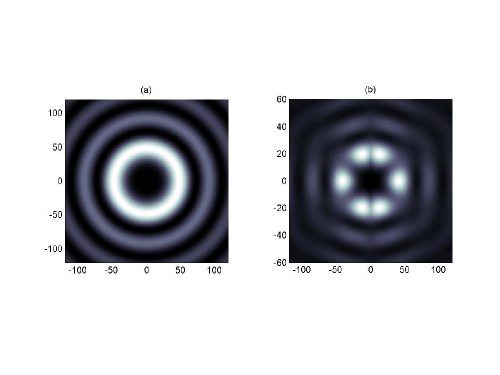
Figure 1: Intensity pattern of an incident Bessel beam of order $m=2$ impinging a calcite crystal at an angle $\alpha=\pi/3$ as seen in a plane (a) perpendicular to the main axis of propagation and (b) parallel to the interface (notice the change of scale). The beam is circularly polarized, ${\cal E}=i{\cal B}$, and $\zeta=\pi/36$. The width of the observation window is measured in units of $\lambda=c/\omega$

.

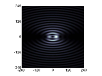
Figure 2: Intensity pattern of the reflected beam resulting from an incident Bessel beam of order $m=2$ with the same configuration as described in Fig. 1. The plane of observation is tilted to be perpendicular to the main direction of propagation. This beam has an intensity pattern invariant under propagation along that axis. The width of the observation window is measured in units of $\lambda=c/\omega$.

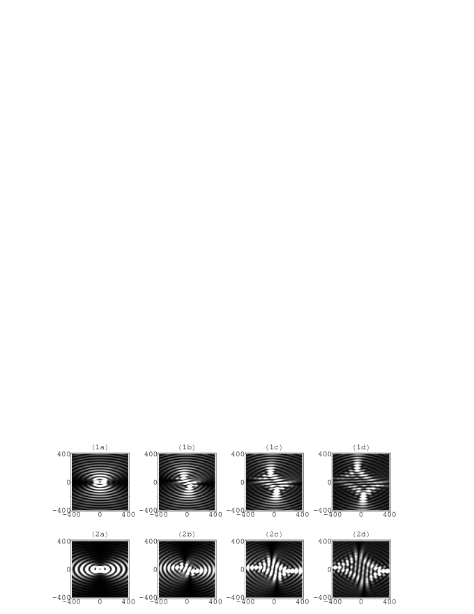
Figure 3: Intensity pattern of the ordinary (1st row) and extraordinary (2nd row) beams resulting from an incident Bessel beam of order $m=2$ with the same configuration as described in Fig. 1. The beam intensity pattern shows a richer topological structure as it propagates. The width of the observation window is given in units of $\lambda=c/\omega$. In Figures (a), the observation plane is the interface itself; in the other figures, it is tilted to be perpendicular to the main propagation axis and is located at: (b)$z=3500$ $\lambda$; (c)$z=7000$ $\lambda$; (d) $z=10500$ $\lambda$.

Figure (1) illustrates the intensity pattern of a Bessel wave in a plane perpendicular to the mean direction of propagation and in a plane parallel to the interface. The corresponding intensity patterns of the reflected, ordinary and extraordinary beams for a calcite crystal ($\epsilon$ = 2.748964, $\epsilon_{\parallel}$ = 2.208196) are illustrated in Figs.(2-3). In these examples, the second order ($m=2$) incident Bessel beam is taken at almost the paraxial limit $\zeta=\pi/36$, the incidence angle is $\alpha=\pi/3$ and the incident wave is a linear superposition of a transverse electric and a transverse magnetic beam with equal amplitudes and a $\pi/2$ phase difference: ${\cal E}=i{\cal B}$. The intensity pattern of the reflected beam (Fig. 2), at the usual angle $\alpha_{R}=-\alpha$, is similar to that of the incident one. As mentioned above, it is invariant under propagation and exhibits an elliptic-like symmetry. The ordinary and extraordinary waves are illustrated in Figs.  (3); for both refracted waves, it is possible to identify an axis of symmetry, though the beams are not propagation invariant. A textbook result is that for a plane wave, the refraction angles of the ordinary and extraordinary waves, $\alpha^{PW}_{O}$ and $\alpha^{PW}_{E}$ respectively, are given in our case by

$$\sin\alpha^{PW}_{O}=\frac{\sin\alpha}{\sqrt{\epsilon\mu}}$$ (50)

$$\sin\alpha^{PW}_{E}=\frac{\sin\alpha}{\sqrt{\epsilon\mu+(\Delta\epsilon/\epsilon_{\parallel})\sin^{2}\alpha}}~{}.$$ (51)

However, for a Bessel beam, the incident wave is a superposition of plane waves propagating in a cone with an aperture given by the axicon angle $\zeta$; it is only in the limit $\zeta\rightarrow 0$ that the above equations define the correct angle for the axis of symmetry $\alpha_{O}$ and $\alpha_{E}$. In general, no analytical expression for an average value of $\alpha_{O}$ and $\alpha_{E}$ could be found.

The intensity patterns (1a) and (2a) in Fig. (3) are given at the interface surface, and all the other patterns are evaluated on planes perpendicular to the main propagation axis of each wave. The latter were obtained performing the corresponding rotations for the observation points and electric fields. The intensity patterns of the ordinary and extraordinary beams have a structure similar to that of the reflected wave near the interface, but this structure gets gradually more complex as they propagate.

Since in this example the ordinary, extraordinary and reflected electric fields are approximately contained in a plane perpendicular to their main direction of propagation, the topological structure of their polarization can be studied using Stokes parameters nye ; these are defined as

$$S_{0} = |E_{x}|^{2}+|E_{y}|^{2}$$

$$S_{1} = |E_{x}|^{2}-|E_{y}|^{2}$$

$$S_{2} = E^{*}_{x}E_{y}+E_{x}E^{*}_{y}$$

$$S_{3} = -i(E^{*}_{x}E_{y}-E_{x}E^{*}_{y})~{},$$

and are given in terms of light intensities for different orientations of an analyzer. The condition $S_{3}({\bf x})=0$ corresponds to local linear polarization at the point ${\bf x}$, and $S_{1}({\bf x})=S_{2}({\bf x})=0$ to circular polarization. A polarization singularity corresponds to $S_{1}({\bf x})=S_{2}({\bf x})=S_{3}({\bf x})=0$. Since $S_{0}=S_{1}^{2}+S_{2}^{2}+S_{3}^{2}$, this condition gives a zero intensity point where polarization is not well defined.

Performing such an analysis on the incident, reflected and refracted beams, we found extended regions where the reflected and refracted beams are approximately linearly polarized if the incident beam is circularly polarized in the sense that ${\cal E}\simeq\pm i{\cal B}$; this is illustrated in Figs. (4-6). As expected, the polarization of the ordinary beam is orthogonal to that of the extraordinary beam. The behavior of the polarization singularities is quite interesting: for the incident beam, an optical vortex is located at its center so that ${\bf E({\bf 0})\times\hat{e}_{q}}={\bf 0}$. But neither the refracted nor the reflected beams are null at that point: this means that a polarization vortex may not survive the reflection and refraction process. However, $S_{0}=0$ at other locations both at the interface and along the produced beams and, in fact, the number of these singularities increases as the refracted beams evolve. This phenomenon is similar to that described in Ref. flossmann ; flossmann2 for a Laguerre-Gaussian beam.

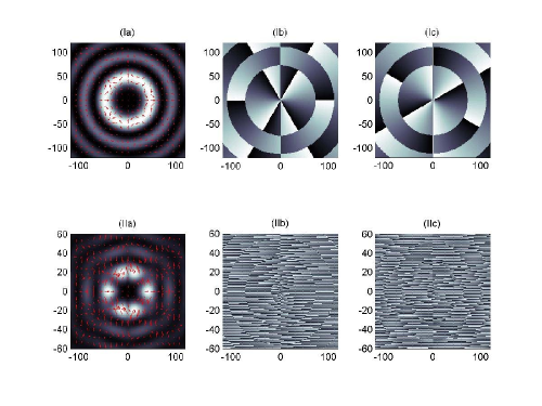
Figure 4: (Color on line) Intensity, polarization and phase patterns for a Bessel beam of order $m=2$ with ${\cal B}=i{\cal E}$ and $\zeta=\pi/36$. The patterns are produced in a plane perpendicular to the main axis of propagation (upper row) and at an angle $\alpha=\pi/3$ with that axis (lower row). The second and third columns show the density plot of the phase for the electric field along two perpendicular vectors on the corresponding plane. The brighter (darker) regions correspond to phases close to $\pi$ ($-\pi$). The unit of length is $\lambda=c/\omega$.

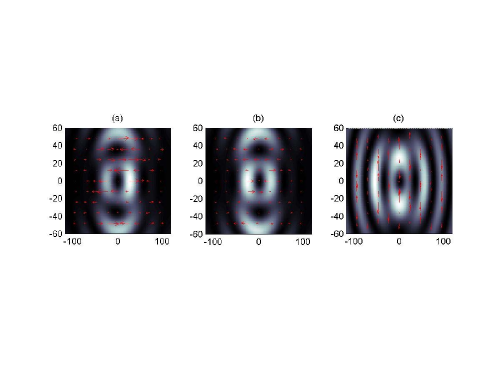
Figure 5: (Color on line) Intensity and polarization patterns for the reflected, ordinary and extraordinary beams at the interface resulting from an incident Bessel beam of order $m=2$ with the same configuration as described in Fig. 1. Notice the different scales. The observation window dimensions are given in units of $\lambda=c/\omega$.

Given the analytic expressions, the phase patterns can be easily analyzed for each component of the electric field. Such an analysis is essential for the understanding of the mechanical properties of the beams. For a Bessel beam of order $m$, Eq. (37) implies that the components $E_{i}$ are superpositions of fields with phase $m^{\prime}\phi+k_{z}z$, where $m^{\prime}=m,m\pm 1$. The linear momentum density along the $z$ direction is proportional to $k_{z}$ and the term proportional to $\phi$ determines the orbital angular momentum density along that axis, which is given by the formula

$${\cal L}_{z}=\frac{1}{4\pi}\sum_{i=x,y,z}E_{i}[\frac{\partial}{\partial\phi}]A_{i}.$$ (53)

Accordingly, phase vortices with a topological charge $m$ contribute to the orbital angular momentum with a factor proportional both to $m$ and to the moduli of the corresponding electric field components. For reference, the phase patterns of a $m=2$ Bessel beam for two perpendicular components of the electric field in two distinct planes are shown in Fig. (4): one perpendicular to the main axis of propagation (first row) and another at an angle $\alpha=\pi/3$ with the former (second row). In the first row, the standard $m^{\prime}=1,2,3$ optical charge vortices are observed, but in the second row the phase patterns exhibit an extremely complex topological structure (dislocations, vortices and bifurcations) on both short and long length scales of order $1/k_{z}$ and $1/k_{\bot}$ respectively. It is also worth noticing that the electric field perpendicular to the tilted plane is not negligible.

The reflected, ordinary and extraordinary beams just at the interface posses, as expected, a phase structure qualitatively similar to that shown in Fig. 4 in the (IIb) and (IIc) plots. In particular, the reflected wave exhibits an elliptic-like symmetry with phase vortices in the plane perpendicular to its axis; this is shown in the first row of Fig. (6).

Due to the anisotropy inside the crystal, the only component of the angular momentum that can be conserved is the one along the crystal axis a-m-i ; its density is given by

$${\cal L}_{z}=\frac{1}{4\pi}\sum_{i=x,y,z}D_{i}[\frac{\partial}{\partial\phi}]A_{i}.$$ (54)

where ${\bf D}$ is the electric displacement vector. If the ordinary and extraordinary beams do not propagate along the crystal axis, their angular momentum along their propagation axis is not conserved. This in turn should be manifested as the creation and annihilation of phase vortices as the beams propagate in the crystal. In the second and third rows of Fig.(6) the phase diagrams for the ordinary and extraordinary beams are illustrated at planes located deep inside the crystal: both beams have a rich topological structure but the characteristic length is much smaller for the extraordinary wave. Notice that for both ordinary and extraordinary waves, there is a strong correlation between the phase diagrams and the intensity patterns.

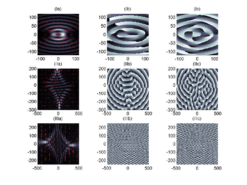
Figure 6: (Color on line) Intensity, polarization and phase patterns for the reflected (1st row), ordinary (2nd row) and extraordinary (3rd row) beams resulting from an incident Bessel beam of order $m=2$ with the same configuration as described in Fig. 1. The plane of observation is perpendicular to the main axis of propagation of each beam and is located at a distance $10500\lambda$ from the interface plane. The brighter (darker) regions correspond to phases close to $\pi$ ($-\pi$). Unit of length is $\lambda=c/\omega$. Notice the different coordinate scales.

IV Conclusions

In this work, explicit formulas have been obtained that permit an analytic treatment of birefringence in uniaxial crystals. These expressions are valid for arbitrary orientations of the incident beam and the axis of the crystal with respect to the plane defining the interface. An illustrative application has been worked out in detail for a Bessel beam and a particular orientation of the crystal axis: it has shown that the electric fields of ordinary, extraordinary and reflected waves take a relatively simple analytic form in terms of a circuit integral. With these results, it was shown that the polarization and phase vortices of the ordinary and extraordinary beams evolve into a complex structure for sufficiently thick crystals. This structure is quite different for the ordinary and extraordinary beams and necessarily leads to different mechanical properties of the field. In was also shown that the reflected beam has elliptic symmetry, exhibits phase and polarization vortices and is invariant under propagation. We expect these results to be useful for the correct characterization of general waves in birefringent crystal as they are widely used at present in optical experiments.

References

• (1) C. Huygens, Traité de la lumière, Chap. V, (1690). An english translation is available at ¡http://www.gutenberg.org/etext/14725¿.
• (2) I. Newton, Opticks, Queries 25-28 (Second English Edition, 1718). Reprinted by Dover (New York, 1979).
• (3) J. Lekner, J. Phys: Condens. Matter 3, 6121 (1991).
• (4) J. A. Fleck and M. D. Feit, J. Opt. Soc. Am. 73, 920 (1983).
• (5) R. Martínez-Herrero, J. M. Movilla, and P. M. Mejías, J. Opt. Soc. Am. A 18, 2009 (2001).
• (6) A. Ciattoni, G. Cincotti, and C. Palma, J. Opt. Soc Am. A 19, 1422 (2002).
• (7) A. Ciattoni, G. Cincotti, and C. Palma, J. Opt. Soc Am. A 19, 792 (2002).
• (8) A. Ciattoni and C. Palma, Opt. Comm. 224, 175 (2003).
• (9) J. Durnin, J. Opt. Soc Am. A 4 651 (1987); Z. Bouchal and M. Olivik, J. Mod. Opt. 42, 1555 (1995); Z. Bouchal, R. Horák, and J. Wagner, J. Mod. Opt. 43, 1905 (1996); R. Horák, Z. Bouchal, and J. Bajer, Opt. Comm. 133, 315 (1997).
• (10) J. Durnin, J. J. Miceli, and J. H. Eberly, Phys. Rev. Lett. 58, 1499 (1987); J. Turunen, A. Vasara and A. T. Friberg, Appl. Opt. 27, 3959 (1988); R. M. Herman and T. A. Wiggins, J. Opt. Soc. Am. A 8, 932 (1991); K. Thewes, M. A. Karim, and A. A. Awwal, Opt. Laser Technol. 23, 105 (1991); N. Davidson, A. A. Friesen, and E. Hasman, Opt. Commun. 88, 326 (1992); G. Scott and M. McArdle, Opt. Eng. 31, 2640 (1992); J. A. Davis, J. Guertin, and D. M. Cottrell, Appl. Opt. 32, 6368 (1993); J. Arlt and K. Dholakia, Opt. Commun. 177, 297 (2000); A. Flores-Pérez, J. Hernández-Hernández, R. Jáuregui, and K. Volke-Sepúlveda, Opt. Letts. 31, 1732 (2006).
• (11) J. F. Nye, Proc. Roy. Soc. Lond. A 389, 279 (1983); M. V. Berry and M. R. Dennis, Proc. Roy. Soc. Lond. A 456, 2059 (2000).
• (12) D. Rozas, C. T. Law, and G. A. Swartzlander, Jr., J. Opt. Soc. Am. B, 14, 3054 (1997).
• (13) F. Flossmann, U. T. Schwarz, M. Maier, and M. R. Dennis, Phys. Rev. Lett. 95, 253901 (2005).
• (14) F. Flossmann, U. T. Schwarz, M. Maier, and M. R. Dennis, Opt. Express 14 11411 (2006).
• (15) H. H. Arnaut and G. A. Barbosa, Phys. Rev. Letts. 85, 286 (2000); M. Martinelli, J. A. O. Huguenin, P. Nussenzveig, and A. Z. Khoury, Phys. Rev. A 70, 013812 (2004); C. I. Osorio, G. Molina-Terriza, and J. P. Torres, Phys. Rev. A 77, 015810 (2008).
• (16) A. Nisbet, Proc. Roy. Soc. A 240, 375 (1957).
• (17) S. Hacyan and R. Jáuregui, J. Phys. B: At. Mol. Opt. Phys. 39, 1669 (2006).
• (18) A. Ciattoni, G. Cincotti and C. Palma, Phys. Rev. E 67, 036618(2003).