Frequency-dependent Chemolocation and Chemotactic Target Selection

Abstract

Chemotaxis is typically modeled in the context of cellular motion towards a static, exogenous source of chemoattractant. Here, we propose a time-dependent mechanism of chemotaxis in which a self-propelled particle (e.g., a cell) releases a chemical that diffuses to fixed particles (targets) and signals the production of a second chemical by these targets. The particle then moves up concentration gradients of this second chemical, analogous to diffusive echolocation. When one target is present, we describe probe release strategies that optimize travel of the cell to the target. In the presence of multiple targets, the one selected by the cell depends on the strength and, interestingly, on the frequency of probe chemical release. Although involving an additional chemical signaling step, our chemical “pinging” hypothesis allows for greater flexibility in regulating target selection, as seen in a number of physical or biological realizations.

1 Introduction

Organisms that employ chemical signaling for functions such as antimicrobial defense mechanisms [1, 2, 3] and nutrient uptake [4, 5] must coordinate the influences of a complicated spatio-temporal mixture of signaling molecules emanating from possibly many sources. A fundamental problem in chemotaxis is how the cell determines a strategy to best select a specific target from many? This problem arises for many chemotactic organisms, such as E. coli [6], Myxococcus xanthus  [7], and Dictyostelium discoideum [8], and poses a challenging theoretical question.

Here, we propose a biologically plausible mechanism involving active sensing, in which chemical signaling is initiated by a chemical prompt from the chemotactic cell. Potential biological manifestations of active sensing include “diffusion sensing” [9] and cancer cell chemotaxis [10]. Diffusion sensing is a particular variant of quorum sensing that involves release of a metabolically inexpensive compound, inducing nearby cells to emit the main signal back to the first cell indicating to it that that other chemically responsive targets are in the vicinity [9]. Cancer cells also exploit this type of indirect sensing by producing excess amounts of matrix metalloproteinases (MMP) which cleave substrates (such as growth factors and laminins) bound to the extracellular matrix (ECM) [10]. These cleavage products diffuse back to the cancer cells, inducing their chemotaxis. Dynamic multistep chemotaxis mechanisms may also arise in the mating of yeast, where each sex of yeast emits its own pheromone that up-regulates gene expression of the complementary pheromone in the opposite sex [11].

In our model of active sensing, moving chemical sources and targets interact through the time-dependent diffusion of signaling molecules Therefore, the timing of the release and detection of chemoattractants will also be important in the overall chemotactic process [12]. Indeed, there is evidence that the probe emission of MMP’s is transcriptionally regulated and is time-dependent [13]. Experiments have also demonstrated the existence of robust and tunable oscillations in transcription in E. coli [14] and mammalian cells [15], and cAMP release in Dictyostelium discoideum [8, 16]. Another important virtue of the proposed dynamic sensing mechanism is that it allows cells to detect local, transient chemoattractant gradients in complex media where steady-state gradients cannot be sustained. For example, branched, “dead-end” volumes with impenetrable boundaries cannot support a steady-state chemical gradient, but can allow a transient gradient. Therefore, chemotaxis under time-dependent, and in particular, time periodic conditions are realizable systems for further exploration.

Basic models for these potentially novel time-periodic chemotactic systems are currently lacking. Here, we distill the extracellular components of a dynamic multistep chemotaxis mechanism into an essential physical model that describes gradient-guided cellular motion towards chemically responsive targets. Classic chemotaxis models by Keller and Segel [17], and their extensions [12, 18] consider passive sources of a chemoattractant to which a cell responds, or consumption of a passive chemical [19]. Contrary to the classic model of chemotaxis where the cell moves along a static chemical gradient of nutrients already present in the environment, we consider the following scenario. Initially, a cell sends out a chemical probe signal (species $a$), which diffuses to stationary targets. Upon contact with the targets, the probe chemical $a$ induces the target to release a different chemical (species $b$), which diffuses back to the cell. In response, the cell moves up the chemical gradient of the chemoattractant $b$. A schematic of our proposed “chemolocation” mechanism, a diffusive analogue of sonar, is shown in Fig. 1, where one cell and two targets are depicted. Here, we assume that chemoattractant $b$ is different from probe chemical $a$ (“paracrine” signaling) and that the cell uses only $b$ to guide its motion towards the target(s).

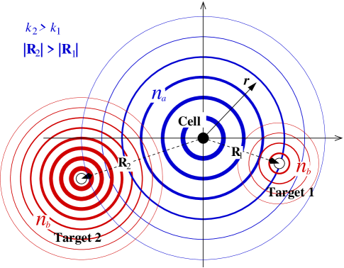
Figure 1: A schematic of a motile cell releasing probe chemical $a$ (blue) which gets converted at fixed targets to a chemoattractant $b$ (red) which the cell detects and uses to move. For the two target case shown here, the initially farther Target 2, has a larger $a\rightarrow b$ conversion rate ($k_{2}>k_{1}$).

2 Mathematical Model

Denote the concentrations at spatial position ${\bf r}$ of probe chemical $a$ emitted by the cell, and chemoattractant $b$ produced by the fixed targets by $n_{a}({\bf r},t)$ and $n_{b}({\bf r},t)$, respectively. The production of chemoattractant $b$ by the targets may be initiated by binding of probe $a$ to receptors on the targets. Although the cell needs to detect spatial gradients in $n_{b}$, we assume for simplicity that both the cell and the target can be treated as point particles when considering the diffusive dynamics of $n_{a}$ and $n_{b}$.

The governing equations in our model are

$$\dot{n}_{a}({\bf r},t)=D_{a}\nabla^{2}n_{a}-\mu_{a}n_{a}+F(t)\delta({\bf r}-{\bf R}(t)),$$ (1)

$$\dot{n}_{b}({\bf r},t)=D_{b}\nabla^{2}n_{b}-\mu_{b}n_{b}+\sum_{j}\!\delta({\bf r}-{\bf R}_{j})K_{j}\!\left[n_{a}({\bf r},t-t^{\prime}),t\right],$$ (2)

$$\dot{\bf R}(t)=\int_{-\infty}^{t}\gamma(t^{\prime})\nabla U[n_{b}({\bf r},t-t^{\prime})]\mbox{d}t^{\prime}\big{|}_{{\bf r}={\bf R}(t)}$$ (3)

where $\delta(\cdot)$ is the Dirac delta function, ${\bf R}(t)$ is the position of the moving cell, ${\bf R}_{j}$ are the fixed target positions, $D_{a},D_{b}$ are the uniform probe and chemoattractant diffusivities, and $\mu_{a},\mu_{b}$ their uniform degradation rates. In Eq. 1, $F(t)$ represents the time-dependent emission of probe chemical $a$ by the cell at position ${\bf R}(t)$, while in Eq. 2 the term $\sum_{j}\delta({\bf r}-{\bf R}_{j})K_{j}\left[n_{a}({\bf r},t-t^{\prime}),t\right]$ represents the total production of $b$ from $a$ by all the targets $j$, each at fixed position ${\bf R}_{j}$. Note that for systems in dimension $d\leq 2$, we must assume $\mu_{a},\mu_{b}>0$ if $F(t\rightarrow\infty)>0$ in order for the chemical concentrations to remain bounded. The functional $K_{j}\left[n_{a}({\bf R}_{j},t-t^{\prime}),t\right]$ embodies all chemical steps in the production of chemoattractant $b$ in response to contact with probe chemical $a$. The production of chemoattractant $b$ occurs with a delay $t^{\prime}$, (the time taken for a single or multi-step reaction along the signaling pathway) after the targets are exposed to the probe $a$ at a time $t-t^{\prime}$  [4, 20]. We will henceforth assume the simplest model for the kernel $K_{j}\left[n_{a}({\bf R}_{j},t-t^{\prime}),t\right]=k_{j}n_{a}({\bf R}_{j},t)$, representing instantaneous production, with rate $k_{j}$, of chemoattractant proportional to the concentration of probe.

Equation 3 describes the motion of the cell in an effective time-dependent potential $U\left[n_{b}({\bf R}(t),t)\right]$ generated by the dynamics of the chemoattractant $n_{b}({\bf R}(t),t)$. The functional $U\left[n_{b}({\bf r},t)\right]$ could be a nonlinear function of $n_{b}({\bf r},t)$, such as one with threshold and saturation like $U\propto n_{b}^{\alpha}({\bf r},t)/(\textrm{const.}+n_{b}^{\alpha}({\bf r},t))$, where $\alpha$ is the Hill coefficient. This form may be more appropriate when cooperative binding of many chemoattractant molecules is required to trigger cellular migration. The response $\gamma$ itself may also be time-dependent. Also, note that not only might the production of chemoattractant $b$ encounter a delay, the cell response embodied by $\gamma$ might be also delayed. Although such delayed and nonlinear responses may result in intrinsically rich signaling behavior, for the sake of simplicity, and in order to analyse our results with as few free parameters as possible, we assume the “force” on the cell is proportional to the local chemoattractant gradient i.e.,

$$\dot{{\bf R}}(t)=\gamma\nabla n_{b}({\bf r},t)\big{|}_{{\bf r}={\bf R}(t)},$$ (4)

Stochastic effects due to low $n_{a},n_{b}$ concentrations or other random effects within the signaling process [21] can also be easily incorporated component by either considering a randomly varying $\gamma(t)$ and/or by adding a random noise to Eq. 3 or 4. The additive noise is equivalent to endowing the cell with Brownian motion. Nonetheless, we show that even in the ideal case of perfect signaling and constant $\gamma$, novel target selection phenomena arise.

In the following analysis, we define dimensionless parameters by measuring length in units of the initial separation $R_{*}$ between the probe and its farthest target, and time in units of $(R_{*})^{2}/D_{a}$. In spatial dimension $d$, the dimensionless equations are identical in form to Eqs. 1-3 except with $D_{a}\equiv 1$, and the terms $D_{b},\mu_{a,b},k_{j},\gamma$, and $F(t)$ replaced by $D_{b}/D_{a}$, $\mu_{a,b}R_{*}^{2}/D_{a}$, $k_{j}/(D_{a}R_{*}^{d-2})$, $\gamma/(D_{a}R_{*}^{d})$, and $R_{*}^{2}F(t)/D_{a}$, respectively.

The solutions to Eqs. 1 and 2 can be solved in terms of Green’s functions and the cell position ${\bf R}(t)$. Upon substitution of $n_{b}$ into Eq. 4, we find a self-consistent nonlinear equation for the cell position

$$\dot{{\bf R}}(t)=\gamma\sum_{j}k_{j}\int_{0}^{t}\mbox{d}t^{\prime}\int_{0}^{t^{\prime}}\mbox{d}t^{\prime\prime}F(t^{\prime\prime})G_{a}({\bf R}(t^{\prime\prime})-{\bf R}_{j};t^{\prime}-t^{\prime\prime}){\bf H}_{b}({\bf R}(t)-{\bf R}_{j};t-t^{\prime}),$$ (5)

where $G_{a}({\bf r};t)=(4\pi t)^{-d/2}e^{-r^{2}/4t}e^{-\mu_{a}t}$, and

$$\begin{array}[]{l}{\bf H}_{b}({\bf R}(t)-{\bf R}_{j};t-t^{\prime})\equiv\nabla G_{b}({\bf r}-{\bf R}_{j};t-t^{\prime})\big{|}_{{\bf r}={\bf R}(t)}\\[13.0pt] \displaystyle\hskip 28.45274pt=\displaystyle{2\pi({\bf R}_{j}-{\bf R}(t))e^{-|{\bf R}(t)-{\bf R}_{j}|^{2}/[4D(t-t^{\prime})]}e^{-\mu_{b}(t-t^{\prime})}\over[4\pi D(t-t^{\prime})]^{d/2+1}}.\end{array}$$ (6)

Although the model equations are linear in $n_{a},n_{b}$, the moving source of probe chemical renders the problem intrinsically nonlinear and not amenable to analytic treatment. Since bounds and analytic expressions for $n_{b}({\bf r},t)$ and ${\bf R}(t)$ can be found only in special cases (such as $F(t)\propto\delta(t)$), we will solve for the cell trajectory by either numerically integrating Eq. 5, or by directly numerically solving Eqs. 1-3 on a fixed lattice using a stable backward-time, central space scheme with step sizes $\Delta x=\Delta t=10^{-3}$. in this case, the system boundary is chosen to be far enough away from the targets as to be irrelevant. We have verified that our results do not depend on the numerical approach employed.

3 Results and Discussion

We shall study our model predominately by solving either Eqs. 1-3 or Eq. 5 numerically, and exploring the qualitative features of the chemolocation mechanism. However, in certain physical limits, we find analytical relationships useful in describing target selection.

3.1 Single Target

In biological media or in laboratory realizations [22], diffusion often occurs in confined or ramified geometries. For chemotaxis across capillaries, or across percolating paths, the effective dimensionality $d$ of the diffusion process may be smaller than the spatial dimension. For simplicity, we first explore the qualitative behavior of the one-dimensional ($d=1$ and ${\bf R}(t)\equiv X(t)$) version of our model with initial condition $n_{a}(x,0)=n_{b}(x,0)=X(0)=0$, and $\gamma=1$. As a demonstration of the chemolocation mechanism, consider a cell moving towards a single target under different probe release protocols $F(t)$. Different strategies of probe release qualitatively influence the ability of the cell to reach the target.

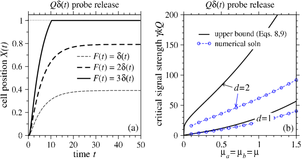
Figure 2: Chemolocation to a single target using a single $\delta$-function probe release. (a) Motion of the probe towards a single target in $d=1$ using three different $\delta$-function release intensities. Delta-functions were approximated with releases of duration $\mbox{d}t=0.1$. Parameters used were $D=\gamma=k=1$ and $\mu_{a}=\mu_{b}=0.1$. (b) Critical signaling strength $\gamma kQ$ as a function of chemical decay rates $\mu=\mu_{a}=\mu_{b}$. Results from numerical solutions and the upper bound Eq. 8 are shown for both $d=1$ and $d=2$.

Figure 2 shows the trajectories and maximum distance traveled by the cell when a single $\delta$-function probe is emitted at $t=0$. Here, and in the rest of the paper, the “$\delta$-function” is approximated by a narrow square pulse release of duration $\mbox{d}t=0.1$ and intensity $Q$. The cell starts to move only after a short delay during which some of the probe has reached the target, and the converted chemoattractant has diffused back to the cell. For a single impulse release of probe $a$, the velocity of the cell towards the target is initially high but eventually goes to zero since the system runs out of the chemoattractant $b$ once the single pulse of probe $a$ has dissipated. Thus, for a modest (e.g. $Q=1,2$) single-pulse release in Fig. 2(a), the cell moves only part of the distance to the target. In the low mobility (small $\gamma$) limit, an approximation to the total travel distance $X_{\infty}$ after probe release in a single pulse can be obtained by setting ${\bf R}(t^{\prime\prime})={\bf R}(t)=0$ in Eq. 5. In one-dimension ($d=1$), integrating the left-and-side of Eq. 5 yields $\int_{0}^{\infty}\dot{X}(t)\mbox{d}t=X_{\infty}$. Explicit evaluation of the time integral of the right-hand-side of Eq. 5 shows that

$$X_{\infty}>{Q\gamma\over 4D\sqrt{\mu_{a}}}\sum_{j}k_{j}{X_{j}\over|X_{j}|}e^{-\left(\sqrt{\mu_{a}}+\sqrt{\mu_{b}/D}\right)|X_{j}|}.$$ (7)

When there is only a single target at $X_{1}=1$, Eq. 7 gives a lower bound for $X_{\infty}$, implying that

$$\gamma kQ\geq 4D\sqrt{\mu_{a}}e^{\sqrt{\mu_{a}}+\sqrt{\mu_{b}/D}}\quad(d=1)$$ (8)

is a sufficient condition for the cell to reach the target. The analogous sufficient conditions for insuring the cell reaches a single target in $d=2$ and $d=3$, are

$$\gamma kQ\geq{4\pi^{2}\over\sqrt{\mu}K_{0}(\sqrt{\mu})K_{1}(\sqrt{\mu})}\quad(d=2),$$ (9)

and

$$\gamma kQ\geq{16\pi^{2}e^{2\sqrt{\mu}}\over\sqrt{\mu}+1}\quad(d=3),$$ (10)

respectively. These “critical” values of the signalling strength $\gamma kQ$ represent the analytically obtainable lowest values above which the target is acquired with certainty. For $d=2,3$, these conditions derived from the ${\bf R}(t^{\prime\prime})={\bf R}(t)=0$ approximation are independent of the relative diffusivity $D$. In higher dimensions, the spreading of probe and chemoattractant concentrations in more severe so that under the approximation ${\bf R}(t^{\prime\prime})={\bf R}(t)\approx 0$, the stationary cell experiences a significantly diminished gradient compared to that which it experiences if it had moved. Chemical decay $\mu$ also diminishes the signal. Therefore, the signalling strength required for reaching the target is significantly increased in this “adiabatic” approximation, especially for large $d$ or $\mu$. Fig. 2(b) plots the critical values (for $d=1$ and $d=2$, $d=3$ not shown) of the signaling strength $\gamma kQ$, from both simulations and Eq. 8, as functions of $\mu=\mu_{a}=\mu_{b}$. Indeed, the sufficient condition Eq. 8 for $d=1$ provides the tightest bound.

The likelihood of arrival to a single target can be enhanced not only by increasing the signaling strength $\gamma kQ$, but also by releasing multiple pulses (as will be shown in Fig. 4(b)) and by releasing probe more slowly. Consider the case where the cell contains a fixed amount of probe chemical $a$. How should the cell release this fixed amount of probe to best reach the target? Suppose the release occurs in a single pulse of duration $\tau$ and amplitude $F_{0}=F(t\leq\tau)$ such that the total amount $Q=F_{0}\tau$ of chemical released is constant. Fig. 3(a) shows trajectories for a cell that releases a fixed amount, $Q$, of chemical $a$ at a constant rate $F_{0}$ over different lengths of time $\tau=Q/F_{0}$. For $F_{0}=20$ and $\tau=1$, the large magnitude, short duration release allows the cell to travel only approximately 90% of the way to the target. In such cases, the cell’s velocity may reach a high value; however, the cell does not reach the target before all chemical signals have dissipated. For lower intensity, but longer duration releases, the cell is better able to reach the target. Qualitatively, this can be understood by noting that a single $\delta$-function release gives a lower bound on the distance $X_{\infty}$ traveled. If the probe is released more slowly, the cell moves slightly closer to the target, amplifying the effect of the probe chemical that is released at later times, because this portion can reach the cell more quickly reducing its decay.

In the limit $\tau\rightarrow\infty$, with fixed $Q=F_{0}\tau$, we can find an upper bound $X_{\infty}^{\rm max}$ for the distance travelled to a single target by integrating Eq. 7 and summing the total distances travelled for each independent increment $\mbox{d}Q=F_{0}\mbox{d}\tau$ of probe release. Assuming $\mu_{a}=\mu_{b}=\mu$, $D=1$, and $X_{1}=1$ for simplicity, we find for $d=1$,

$$X_{\infty}^{\rm max}=1-{1\over 2\sqrt{\mu}}\ln\left(e^{2\sqrt{\mu}}-{\gamma kQ\over 2D}\right),$$ (11)

valid for $0\leq\gamma kQ\leq 2D(e^{2\sqrt{\mu}}-1)$. Therefore, even for infinitely slow release of a fixed amount $Q$ of probe chemical, a necessary condition $\gamma kQ\geq 2D(e^{2\sqrt{\mu}}-1)$ remains, even if the cell can detect arbitrarily low concentration gradients of chemoattractant.

Even if the cell has sufficient probe to reach the target, if the probe is released very slowly, the time required for the cell to reach the target may be large. Fig. 3(b) plots the time $t^{*}$ it takes for the cell to reach the target, as a function of the pulse duration $\tau$. For large signaling strength $\gamma kQ$, the cell reaches its target for all $\tau$, and reaches its target most quickly for very short pulse durations, $\tau$. When the signaling strength $\gamma kQ$ is decreased, the cell reaches its target only when $\tau$ is greater than some critical value, denoted by the vertical asymptotes (dashed lines) in Fig. 3(b). Additionally, there is a value of $\tau$ which minimizes the arrival time $t^{*}$, and approximately satisfies the condition $\tau\approx t^{*}$, indicating that the cell reaches its target in the shortest time when probe chemical $a$ is released over a period $\tau$ nearly equal to its travel time. If we think of probe $a$ as an effective “fuel” that drives the motion of the cell, it is not ideal to have $\tau\ll t^{*}$, because if chemical $a$ stops being released well before the cell reaches its target, the cell will have to rely on a residual, decaying concentration field $b$ to reach its target. On the other hand, if $\tau\gg t^{*}$, the cell will continue to release chemical $a$ after reaching its target, when a faster release of $a$ would have allowed the cell to reach its target more quickly.

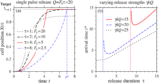
Figure 3: Chemolocation to a single target using a probe pulse of duration $\tau$. (a) Trajectories of a cell to a single target when a fixed, total amount of probe $Q$ is released at a constant rate, $F_{0}$ for a finite time, $\tau$. (b) Arrival times $t^{*}$ of a cell to a single target are plotted as a function of pulse duration $\tau$. Within each curve, the total amount of probe released, $Q$ was held constant. In both plots, parameters used were $D=\gamma=k=\mu_{A}=\mu_{B}=1$.

3.2 Multiple Targets

We now illustrate the mechanism of frequency and response strength-dependent target selection among multiple targets. First consider the one-dimensional case with a cell and two targets. The closer target (at $X_{1}=-0.25$) is assigned a probe-to-chemoattractant production rate $k_{1}=0.5$, while the farther target at $X_{2}=1$ has a larger production rate $k_{2}=1$. Fig. 4(a) shows that when the release of probe chemical is in the form of a Heaviside function, target selection can be controlled by the cell’s response, $\gamma$. For the parameters chosen, if $\gamma=0.1$, the far target is chosen. As the strength of the response is increased beyond approximately $0.225$, the near target is selected by our chemotactic mechanism. When the cell’s response, $\gamma$ is large, the cell is initially pulled strongly towards the near target. Because the distance to the far target increases substantially before the signal from this target reaches the cell, the signal strength diminishes and is insufficient to pull the cell back towards the far target. When the cell’s response is small, the cell is unable to move much towards the near target before the stronger signal from the far target reaches the cell, and the cell ultimately gets pulled to the far target.

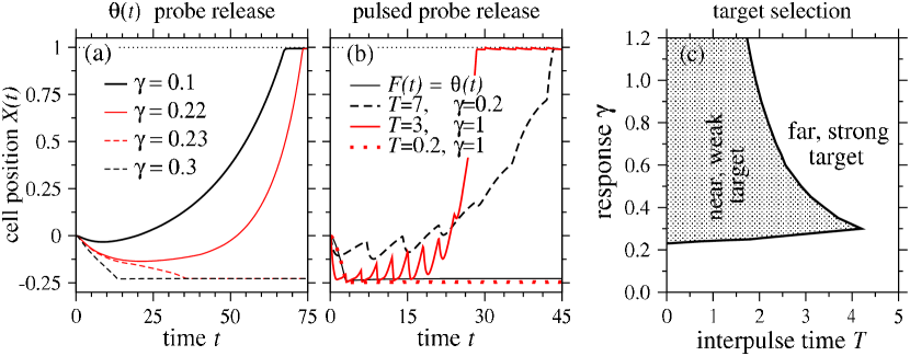
Figure 4: Target selection as a function of chemotactic response $\gamma$ and probe release frequency $1/T$. (a) Response-dependent target selection showing a transition from selecting the further, stronger, target to selecting the weaker, nearer target for a Heaviside release protocol $F(t)=\theta(t)$ and a varying response $\gamma$. When $\gamma\gtrsim 0.235$, the near target is selected, while the far target is selected for smaller $\gamma$. (b) Frequency-dependent target selection, with release protocol $F(t)=T\sum_{i}\delta(t-iT)$ and varied response strength $\gamma$. The weaker nearer target is selected for constant chemical release $F(t)=\theta(t)$ and very high frequency pulsed release $F(t)=0.2\sum_{i}\delta(t-0.2i)$, while the further stronger target is selected for pulsed release at intermediate frequencies (corresponding to interpulse intervals $T=3,7$). These trajectories may first arrive at the nearer target depending upon probe chemical release amplitude. (c) Under the release function $F(t)=T\sum_{i}\delta(t-iT)$, regions of $\gamma-T$ space where the cell reaches the nearer (and weaker), or farther (and stronger) target are shown. When $T\gtrsim 4$, the cell always reaches the far target. For smaller values of $T$, the cell reaches the far target for small and large values of $\gamma$, and reaches the near target for intermediate values of $\gamma$. For all plots, the target strengths are $k_{1}=0.5$, $k_{2}=1$, the decay rates are $\mu_{a}=\mu_{b}=0.1$ and $D=1$. The initial separations between the cell and the targets are $|X_{1}|=0.25$ and $|X_{2}|=1$ respectively.

Target selection can depend not only on probe release intensity and response strength, but is also modulated release frequency. Fig. 4(b) illustrates target selection when the probe chemical is released either as a Heaviside function $\theta(t)$, or as a series of pulses $F(t)=T\sum_{i}\delta(t-iT)$ with an interpulse interval $T$ and varying response $\gamma$. This form of $F(t)$ compares release protocols with equal long-time-averaged probe release. For the parameters chosen, the constant release $F(t)=\theta(t)$ results in the cell arriving at the near target. For pulsed release with interpulse interval $T=3,7$, the cell initially moves towards, and depending on the pulse intensity, may first reach the near target before eventually being pulled to the farther, stronger target. If the release frequency is increased even further, (interpulse interval $T=0.2$, red dotted curve), the trajectories will again arrive at the closer, weaker target. Since the underlying processes are dissipative, at very high frequencies, the cell cannot respond fast enough to distinguish the pulses and a rapid succession of pulses is equivalent to an effective-amplitude, constant emission.

In Fig. 4(c), we show a phase diagram indicating the regions of $\gamma$-$T$ space in which we expect the cell to go to the near, weak target, or to the far, strong target. When the interpulse time $T$ is small and the cell’s response $\gamma$ is small, it will go to the far target. For $\gamma>0.225$, the near target is selected. These results are consistent with those shown in Fig. 4(a). When the interpulse interval $T$ is large, the cell will reach the far target for any response strength $\gamma$. In this example, the cell will reach the far target for any value of $T\gtrsim 4$. When $T$ falls in the interval $0<T<4$, the cell will reach the far target when $\gamma$ is either small or large, but will reach the near target at intermediate values of $\gamma$. When the cell reaches the far target and $\gamma$ is large, initial chemoattractant pulses quickly pull the cell towards the near target. For several pulses, alternating chemoattractant waves from the far and near targets will pull the cell away from, then back towards, the near target. The cell appears to “bounce” around the near target. Eventually, a wave of chemoattractant from the far target will dislodge the cell from the near target, and the next wave of chemoattractant from the near target will be insufficient to return the cell to the near target. After this, each subsequent pulse brings the cell closer to the far target, until the cell reaches this target. The trajectory with parameters $\gamma=1$, $T=3$ illustrates this qualitative behavior in Fig. 4(b). When the cell with small $\gamma$ reaches the far target, it does so without first reaching the near target. The trajectory with parameters $\gamma=0.2$, $T=7$ in Fig. 4(b) illustrates this qualitative behavior.

A more quantitative understanding of the target selection phenomenon can be found in the small $\gamma$ limit, where the cell does not move much under the influence of a single probe pulse (such as the trajectory corresponding to $\gamma=0.2$ and $F(t)=7\sum_{i}\delta(t-7i)$ in Fig. 4(b)). If the cell does not move appreciably under the influence of a single probe pulse, we can use Eq. 7 to approximate the asymptotic distance traveled by the cell as a result of one single probe pulse released at $t=0$. If $X_{\infty}<0$, subsequent probe pulses will be released when the cell is closer to the left target, and the cell will eventually incrementally move leftward. If $X_{\infty}>0$, the cell will ultimately arrive at the right target. Therefore, $X_{\infty}=0$ defines an approximate boundary for selection between two targets in $d=1$.

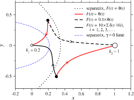
Figure 5: Target selection in $d=2$ depends on probe release protocol. The separatrix corresponding to $\theta(t)$ probe release (dotted line) divides the space such that trajectories (solid red lines) originating from points to the right of the dotted line arrive at the stronger target (big open circle) while those starting from the left arrive at the weaker target (small open circle). Amplitude-dependent target selection is shown by using $F(t)=0.1\times\theta(t)$ (black dashed line), leading to a different target than when $F(t)=\theta(t)$. Likewise, frequency-dependent target selection is demonstrated using $F(t)=10\sum_{i}\delta(t-10i)$ (black solid line with a unit average probe release) where the cell selects the nearer target when started in a region that would normally lead to selection of the stronger, farther target when $F(t)=\theta(t)$. For comparison, the separatrix for continually constant probe release $F$ computed by integrating along the ridge of the static field $n_{b}({\bf r})$ is shown by the thin blue curve. Parameters used were $D=k_{1}=1$, $k_{2}=0.2$, $\mu_{a}=\mu_{b}=0.001$ and $\gamma=10$. The numerical solution to Eqs. 1-3 in $d=2$ were found using the Peaceman-Rachford algorithm.

Generalizing the phenomenon to $d$ dimensions, we expect that for each release sequence $F(t)$, there will be at least one $d-1$ dimensional surface that separates trajectories that evolve to different targets starting from a given initial position on the $d$ dimensional manifold. Figure 5 shows trajectories of cells searching and selecting between two targets in $d=2$. The separatrix associated with the Heaviside probe release $F(t)=\theta(t)$ is indicated by the dotted curve that divides the space such that trajectories originating from the right/left of this line are led to the stronger/weaker target respectively. For comparison, the separatrix for constant probe release for all times (corresponding to the $\gamma\rightarrow 0$ limit) computed by integrating along the ridge of the static field $n_{b}({\bf r})$ is shown by the thin blue curve, highlighting its sensitivity to $F(t)$. We then start the cell within regions where one target is clearly selected when the probe chemical is released with $F(t)=\theta(t)$, but with either a diminished released rate or with pulsed release, such that the average rate of chemical released per unit time is 1. As in the $d=1$ case we find that for Heaviside function release, a larger release rate favors the weaker, closer target, while a smaller release rate favors the stronger, farther target (thick dashed curve). In one dimension we find that slow pulsed release favors the far, strong target over the near, weak target. In contrast, for $d=2$, we find that slow pulsed release favors the near target (solid black curve). This may be understood as follows. In $d=1$, pulsed release causes the cell to quickly go towards the near target, but a subsequent wave of chemoattractant from the far target caused the cell to ultimately select the far target. In two dimensions, the radial divergence of the concentration fields renders the signal from the far target insufficient to pull the cell from the weaker target. In higher dimensions, the radial spread is stronger, and the frequency and $\gamma$-dependent selection mechanism is significantly mitigated.

While nontrivial target selection phenomena still arises in $d=2$, many cellular chemotactic responses, such as development, occur in $d=3$ where the concentration fields spread significantly and attenuate signalling responses. However, in many situations, the medium in which the concentration fields $n_{a}$ and $n_{b}$ diffuse is heterogeneous. A common biological example is the extracellular cellular matrix and the existence of intervening cells and tissues. Diffusive transport in a random medium can also be described by diffusion in a lower, effective dimension. Furthermore, media that is ramified can transport signals in a one-dimensional manner along the main percolating path once side branches have saturated with probe and/or chemoattractant. Therefore, signatures of our proposed mechanism may nonetheless arise in $d=3$.

Although our results are based on a simplified model of response (Eq. 4) where $U[n_{b}({\bf r},t)]\propto n_{b}({\bf r},t)$, and neglect noise of memory effects in $\gamma$, they provide clues into how more complex models might behave. For example, in the limit of a motility response that requires highly cooperative binding of multiple chemoattractants (large Hill coefficient $\alpha$), the motion of the cell would be appreciable only when a very narrow range of gradients in $n_{b}$ cross the cell. High cooperativity imposes a switching response which would lead to saltatory movements of the cell. While larger velocities can be attained (because $\nabla U[n_{b}]$ can be larger is $\alpha$ is large) the time scale over which $\nabla U[n_{b}]$ is large is short. We expect the net effect to be quantitative and that most our qualitative results will persist.

Delayed response, or directional memory, may arise from receptor adaptation and other intermediate steps in the cell signaling pathway [20], and may give rise to behavior that is more difficult to intuit without numerical computations. However, simple conclusions in certain limits can be motivated by comparing the delay time, or directional correlation time with the arrival times of the gradients $\nabla U[n_{b}]$ from the targets. For example, if directional memory is longer than the difference in times it takes for the $n_{b}$ signal to propagate from the close and far targets, the cell would be less sensitive to the signal from the far target. This would have the effect of biasing selection of the near target, provided the release frequency is sufficiently high.

One example of a biologically-motivated variant of our model worth further discussion is “autocrine” signalling. Autocrine signalling is often relevant to bacterial aggregation, where the probe is identical to the chemoattractant ($a=b$). Within our mathematical framework, the autocrine mechanism is described by replacing $n_{b}({\bf r},t)$ with $n_{a}({\bf r},t)$ in Eqs. 2 and 4, and setting $\mu_{b}=\mu_{a}$ and $D_{b}=D_{a}$. This model is also novel in that its naive continuum limit does not map onto existing PDE descriptions such as Keller-Segel type models. In the Keller-Segel model, the production of autocrine chemoattractant is simply proportional to the local cell density and is independent of the probing signal the cells receive. Our qualitative results for paracrine signalling also hold in the autocrine signalling problem, which can be understood by considering the $n_{a}$ profile generated by the cell and that generated by the target. In the autocrine case, when the cell responds to $n_{a}$, its self-produced $n_{a}$ field is maximal near the point where it is released. Therefore, the self-produced $n_{a}$ tends to keep the cell from moving. When the gradient in $n_{a}$ generated from the target is finally felt, the cell will move towards the target; however, typically by this time, the self-generated $n_{a}$ has diffused and/or dissipated away such that it’s “restoring force” is weak. Therefore, we expect that all else being equal, the replacement of $n_{b}$ by $n_{a}$, leads to an overall slightly suppressed chemotactic response.

Finally, analysis of the effects of stochastic responses, implemented through additive Brownian terms to Eq. 3 or 4, or through a time random response coefficient $\gamma(t)$, is beyond the scope of this study. However, it has been shown that in a two-dimensional autocrine mechanism, stochastic effects and chemical decay keep the cells diffusive [18], despite the tendency for all cells and targets to aggregate. Therefore, one might expect that target selection to be suppressed in the presence of sufficient noise.

4 Summary & Conclusions

In conclusion, we have proposed a model for dynamic, multistep chemotaxis that involves chemical communication between cell and targets. Our analysis shows that signalling agents can select among potential targets by controlling the amount of, and frequency at which probe chemical is released. Since our moving source problem is intrinsically nonlinear, we employed numerical calculations to provide evidence of a critical target-switching release amplitude, as well as a window of response strengths $\gamma$ within which a cell chooses the nearer, weaker target over the farther, stronger target that is selected outside this window. This effect arises from a nonlinear interplay between diffusion, decay, and chemoattractant production and depends on the frequency of release. Moreover, we found that for the conditions studied, a constant probe release leads to acquisition of the weaker, nearer target, while low frequency spike release leads to acquisition of the stronger, farther target. At higher frequencies, the cell again approaches the weaker, nearer target since high frequency and constant release give rise to similar spatial-temporal probe distributions due to the averaging nature of the underlying diffusive physics. Our numerical experiments have shown that target selection is observed over a wide range of system parameters, suggesting the chemolocation mechanism may be common in Nature.

Numerous variants of our basic model, such as mobile targets that sense probe chemical, stochastic effects, and delays in the signaling processes can be straightforwardly investigated. In the present work, we assumed the simplest deterministic, instantaneous response in order to avoid introducing excessive number of parameters. Nonetheless, we have argued that many extensions of our underlying model, except sufficiently large noise, are likely to qualitatively preserve the predicted results.

The authors thank M. R. D’Orsogna for helpful discussions. This research was supported by grants from the NSF (DMS-0349195) and the NIH (K25AI058672). SAN acknowledges support from an NSF Graduate Research Fellowship.

References

- [1] Chet I, Fogel S, and Mitchell R (1971) Chemical detection of microbial prey by bacterial predators. it J. Bacteriol. 106:863-867.
- [2] Alberts B, et al., Molecular Biology of the Cell: Fourth edn, (Garland Publishing, New York, 2002).
- [3] Cody CC, et al. (2003) Synergistic Antimicrobial Activity of Metabolites Produced by a Nonobligate Bacterial Predator. Antimicrobial Agents and Chemotherapy 47:2113-2117.
- [4] Bray D Cell Movements: From Molecules to Motility, (Garland Publishing, New York, 1992).
- [5] Berg HC (2000) Motile behavior of bacteria. Physics Today 53:24-29.
- [6] Mittal N, Budrene EO, Brenner MP and van Onuardeen A (2003) Motility of Escherichia coli cells in clusters formed by chemotactic aggregation. Proc. Natl. Acad. Sci. 100:13259-13263.
- [7] Velicer GJ and Yu YN (2003) Evolution of novel cooperative swarming in the bacterium Myxococcus xanthus. Nature 425:75-78.
- [8] Tyson JJ and Murray JD (1989) Cyclic AMP waves during aggregation of Dictyostelium amoebae Development 106:421-426.
- [9] Redfield RJ (2002) Is quorum sensing a side effect of diffusion sensing? Trends in Microbiology 10:365-370; Hense BA et al. (2007) Does efficiency sensing unify diffusion and quorum sensing? Nat. Rev. Microbiol. 5:230-239.
- [10] Egeblad M and Werb Z (2002) New roles for the matrix metalloproteinases in the progression of cancer. Nature Rev. Cancer 2:163-176.
- [11] Wang Y and Dohlman HG (2004) Pheromone Signaling Mechanisms in Yeast: A Prototypical Sex Machine. Science 306:1508-1509.
- [12] Clark DA and Grant LC (2005) The bacterial chemotactic response reflects a compromise between transient and steady-state behavior. Proc. natl. Acad. Sci. USA 102:9150-9155.
- [13] Berry H and Larreta-Garde V (1999) Oscillatory behavior of a simple kinetic model for proteolysis during cell invasion. Biophys. J. 77:655-665.
- [14] Stricker J, Cookson S, Bennett MR, Mather WH, Tsimring LS, and Hasty J. (2008) A fast, robust and tunable synthetic gene oscillator. Nature 456:516-519.
- [15] Tigges M, Marquez-Lago TT, Stelling J, and Fussenegger M. (2009) A tunable synthetic mammalian oscillator. Nature 457:309-312.
- [16] Halloy J, Lauzeral, J, and Goldbeter A (1998) Modeling oscillations and waves of cAMP in Dictyostelium discoideum cells. Biophys. Chem. 72:9-19.
- [17] Keller EF and Segel LA (1971) Model for chemotaxis. J. Theor. Biol. 30:225-234.
- [18] Grima R (2005) Strong-coupling dynamics of a multicellular chemotactic system. Phys. Rev. Lett. 96:128103.
- [19] Dillon R, Fauci L Gaver D (1995) A microscale model of bacteria swimming, chemotaxis and substrate transport. J. theor. Biol. 177:325-340.
- [20] Tu Y, Shimizu TS, and Berg HC (2008) Modeling the chemotactic response of Escherichia coli to time-varying stimuli. PNAS 105:14855-14860.
- [21] Endres RG and Wingreen NS (2008) Accuracy of direct gradient sensing by single cells. PNAS 105:15749-15754.
- [22] Bainer R, Park H, Cluzel P (2003) A high-throughput capillary assay for bacterial chemotaxis. J Microbiol Methods 55:315-319.