TUM-HEP-703/08

Soft-Collinear Effective Theory:
Recent Results and Applications

Thorsten Feldmann

Physik Department, Technische Universität München, James-Franck-Straße 2,
D-85748 Garching, Germany

Soft-collinear effective theory (SCET) has become a standard tool to study the factorization of short- and long-distance effects in processes involving low-energetic (soft) particles and high-energetic/low-virtuality (collinear) modes. In this contribution I give a brief overview on recent results for inclusive and exclusive $B$ decays and on applications in collider physics.

[Contributed to “Quark Confinement and the Hadron Spectrum”, Sep 2008, Mainz, Germany]

1 Factorization and SCET

Our ability to provide precise theoretical predictions for high-energy processes in particle physics heavily relies on the concept of factorization, i.e. the systematic separation of dynamical effects from short and long distances. Especially for strong interactions – if factorization holds – the effects of heavy particles and/or highly virtual radiative corrections can be calculated in perturbative Quantum Chromodynamics (QCD), while the long-distance physics of light quarks and gluons can be encoded in (process-independent) hadronic matrix element of composite operators, which can be further studied using non-perturbative methods. A general feature of factorization is the appearance of a factorization scale $\mu$ that relates the infrared (IR) divergences, appearing in loop corrections to short-distance amplitudes/cross sections, and the ultraviolet (UV) divergences of composite operators defining the long-distance matrix elements, such that the scale dependence cancels to any given order in perturbation theory.

A particularly interesting situation arises in processes like, for instance, $B\to X_{s}\gamma$, where $X_{s}$ denotes a hadronic jet containing a light strange quark with energy of order $m_{b}/2$ and invariant mass of order $\sqrt{\Lambda_{\rm QCD}m_{b}}$. Here, the infrared divergences of the short-distance $b\to s\gamma$ vertex corrections can be identified as coming from quarks and gluons being either soft ($|k^{\mu}|\sim\Lambda_{\rm QCD}$) or collinear to the hadronic jet ($k^{\mu}\parallel p_{X}^{\mu}$). The interactions of the $b$-quark with soft degrees of freedom can be expanded in the small parameter $\Lambda_{\rm QCD}/m_{b}$, and the remaining non-analytic dependence on the $b$-quark mass $m_{b}$ can be calculated within the well-known heavy-quark effective theory (HQET). The presence of additional collinear modes leads to new phenomena [1]:

• The $b\to s$ form factors contain Sudakov double logarithms $\ln^{2}(p_{X}^{2}/m_{b}^{2})$.

• The propagation of a collinear quark in the soft background is described by a jet function.

• The partial rate depends on the residual momentum of the $b$-quark, which is encoded in a so-called shape function (SF), i.e. the parton distribution function (PDF) for the $B$-meson.

Again, the expansion in $1/m_{b}$ can be formalized in terms of an effective theory, SCET [2, 3]. To this end, one includes separate field operators for soft and collinear modes, with soft-collinear vertices being multi-pole expanded according to the power-counting of momenta/wave-lengths in the different light-cone directions [4]. The short-distance coefficient functions and the jet function can be calculated by perturbative matching calculations. The renormalization-group (RG) running in SCET resums the large Sudakov logarithms between the hard scale ($m_{b}$) and the jet scale ($|p_{X}|$) [5], where one finally matches onto (non-local) HQET operators that define the $b$-quark PDF.

2 SCET applications

While SCET originally has been designed to discuss factorization in inclusive and exclusive $B$-decays, it has also led to some new insights in collider physics applications. This includes, the traditional field of QCD jet physics and parton showers (which is discussed in more detail by Christian Bauer in these proceedings), as well as resummation effects in high-energy electroweak processes. In the following, I will present a personal selection of recent results, illustrating the main SCET activities for $B$-decays and collider physics (a good overview can also be obtained from the talks presented at the recent SCET workshop 2008 [6]).

2.1 Inclusive $B$ decays

Factorization theorems (see e.g. [7, 8, 9, 10]) play a key role in the determination of the CKM matrix element $|V_{ub}|$ from inclusive semi-leptonic $B\to X_{u}\ell\nu$ decays, as well as for tests of the Standard Model in rare penguin decays $B\to X_{s}\gamma$. In the former, one becomes sensitive to the SF when applying the constraint $E_{X}-|\vec{p}_{X}|\leq\Delta<M_{D}^{2}/M_{B}\,,$ in order to suppress the background from $b\to c\ell\nu$ decays. In the latter, one is experimentally restricted to sufficiently large photon energies, which again implies large recoil energy to the hadronic jet. In both cases, one ends up with a factorization theorem for the decay spectrum, which schematically reads

$$d\Gamma\sim H\cdot J\otimes S\,.$$ (2.1)

Here $H$ denotes the hard function, obtained from a QCD matching calculation, which is presently known to NNLO accuracy both, for $b\to u\ell\nu$ [12] and $b\to s\gamma$ [13]. Furthermore, $J$ represents the universal jet function in SCET, whose NNLO expression (for massless quarks) has been derived in [14] (for massive quarks, the NLO jet function has been given in [15], see also [16]). It is convololuted with a soft function, $S$, which denotes the $b$-quark SF in HQET, whose 2-loop evolution has been studied in [17]. Sub-leading SFs, entering at the level of $1/m_{b}$ corrections, have been classified in [18]. We should also mention that SF-independent relations between $B\to X_{s}\gamma$ and $B\to X_{u}\ell\nu$ can be obtained by appropriately re-weighting the experimental decay spectra, with weight functions determined from the perturbative short-distance functions in the factorization theorem [19].

2.1.1 The $B$-meson shape function

For the community of this workshop, the perhaps most interesting ingredient is the $B$-meson SF, which is defined via the light-cone matrix element (with HQET fields $h_{v}$)

$$\widehat{S}(\hat{\omega}=\bar{\Lambda}-\omega)=\langle B|\bar{h}_{v}\,\delta(\omega-in\cdot D)\,h_{v}|B\rangle\,,\qquad\mbox{($n^{2}=0,\ n\cdot v=1,\ \bar{\Lambda}=m_{B}-m_{b}$)}\,.$$ (2.2)

The SF has support for $0\leq\hat{\omega}\leq\infty$, where large values of the (residual) light-cone momentum $\hat{\omega}$ are described by a radiative tail which can be calculated in perturbation theory.

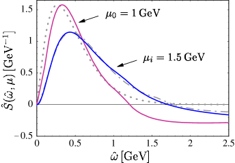
(a)  (b)

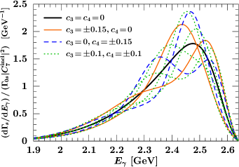
Figure 1: (a) Model SF at low input scale $\mu_{0}=1$ GeV and after evolution (solid lines, figure taken from [10]). For the meaning of the dotted curves and further details, see section 9.2 in [10]. (b) Photon spectrum in $B\to X_{s}\gamma$ resulting from different profile functions in (2.4). Figure taken from [20].

Experimentally, the SF can be directly constrained by the measured photon spectrum in $B\to X_{s}\gamma$ decays (via the above factorization theorem). In addition the moments of the $B\to X_{c}\ell\nu$ spectra determine the HQET parameters $\bar{\Lambda},\mu_{\pi}^{2},\ldots$, which in turn constrain the moments of the SF in a given factorization scheme. For instance, the authors of [10] propose a model-parametrization for the SF at low input scales (in the so-called SF scheme),

$$\widehat{S}(\hat{\omega},\mu_{0})=\frac{N}{\Lambda}\left(\frac{\hat{\omega}}{\Lambda}\right)^{b-1}\exp\left(-b\,\frac{\hat{\omega}}{\Lambda}\right)+\frac{\alpha_{s}}{\pi}\times\mbox{[radiative tail]}\,,$$ (2.3)

where $N$ is a normalization factor, and the free parameters ($b,\Lambda$) can be related to $\bar{\Lambda}$ and $\mu_{\pi}^{2}$. An example is plotted in Fig. 1(a). The ansatz can be compared to the $B\to X_{s}\gamma$ spectrum predicted by the factorization formula.

An alternative approach has recently been proposed in [20]. One starts with the perturbative result for the partonic SF, $\widehat{S}_{\rm part.}(\hat{\omega},\mu_{0})=\delta(\hat{\omega})+\frac{\alpha_{s}}{\pi}\,[\cdots]$, and generates model SFs via

$$\widehat{S}(\hat{\omega},\mu_{0}):=\int dk\,\widehat{S}_{\rm part.}(\hat{\omega}-k,\mu_{0})\,\widehat{F}(k)\,.$$ (2.4)

The profile function $\widehat{F}(k)$ can be directly normalized to HQET parameters and expanded in terms of suitable basis functions; examples are shown in Fig. 1. This procedure is expected to be advantageous for systematic studies of theoretical uncertainties in global fits to $B\to X_{s}\gamma$ spectra and $B\to X\ell\nu$ moments.

2.1.2 Theoretical limitations in $B\to X_{s}\gamma$

In the theoretical discussion of the $B\to X_{s}\gamma$ spectrum, a particular complication arises due to the fact that the weak effective Hamiltonian contains operators that contribute in a different way to the hadronization process, namely the chromomagnetic operator ${\cal O}_{8}(b\to sg)$, and the 4-quark operators ${\cal O}_{1-6}(b\to sq\bar{q})$. At sub-leading order in the $1/m_{b}$ expansion this leads to qualitatively new effects, where the photon does not couple directly to the short-distance $b\to s$ transition. This requires a new type of factorization theorem, which involves a new jet function in the direction opposite to $p_{X}$, as well as new soft functions from operators that are non-local with respect to two light-cone directions [21]. On the one hand, these effects are difficult to estimate (the vacuum insertion approximation leads to corrections of order 5%). On the other hand, they provide a potential mechanism for the observation of CP violating effects, and the leading mechanism for isospin asymmetries between decays of charged and neutral $B$-mesons in this channel.

2.2 Exclusive $B$ decays

SCET applications in exclusive $B$ decays reveal some new aspects compared to the inclusive case. First of all, it has to be realized that the decay into a few light energetic hadrons (with mass $m^{2}\sim{\cal O}(\Lambda^{2})$) is power-suppressed compared to the production of a generic jet (with mass $m_{X}^{2}\sim{\cal O}(\Lambda m_{b})$), since it requires a particular fine-tuning in the phase space of the $B$-meson spectator system. A related subtlety arises from so-called endpoint divergences which prevent the complete (perturbative) factorization of soft and collinear modes (with small invariant mass $\sim m^{2}$). Factorization theorems for exclusive heavy-to-light amplitudes thus take the generic form [22]

$${\cal A}_{i}(B\to MM^{\prime})={\xi_{M}}\cdot T_{i}^{\rm I}\otimes{\phi_{M^{\prime}}}\,+T_{i}^{\rm II}\otimes{\phi_{B}}\otimes{\phi_{M}}\otimes{\phi_{M^{\prime}}}+\ldots\,,$$ (2.5)

where $M,M^{\prime}$ denote light mesons in the final state. Here $T_{i}^{\rm I,II}$ are short-distance functions, where the $T_{i}^{\rm II}$ further factorize into a hard and an exclusive jet function (including spectator scattering), but the $T_{i}^{\rm I}$ do not [25, 28]. Furthermore, $\xi_{M}$ denotes a universal form factor for $B\to M$ transitions, and $\phi_{M,B}$ are light-cone distribution amplitudes (LCDAs) for light and heavy hadrons. Again, $1/m_{b}$ corrections introduce new factorizable and non-factorizable terms. Recent perturbative calculations include NNLO corrections to $T_{i}^{\rm I}$ in non-leptonic $B$ decays [29], NLO spectator scattering in non-leptonic $B$ decays ($T_{i}^{\rm II}$) for tree amplitudes [30] and the leading penguin amplitudes [31], as well as ${\cal O}(\alpha_{s}^{2})$ corrections from ${\cal O}_{7}^{\gamma}$ and ${\cal O}_{8}^{g}$ in $B\to V\gamma$ decays [32]. Below, let us again have a closer look at the non-perturbative ingredients related to $b$-hadrons in the factorization formula (2.5).

2.2.1 Light-cone distribution amplitudes for $b$-hadrons

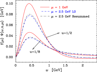
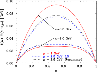
Figure 2: LCDA for $\Lambda_{b}$ as a function of $\omega=\omega_{1}+\omega_{2}$ and $u=\omega_{1}/\omega$ for different scales. Figure from [38].

2-particle LCDAs for $B$-mesons are defined from non-local matrix elements in HQET [33]

$$\langle 0|\bar{q}(z)_{\beta}\,[z,0]\,h_{v}(0)_{\alpha}|B(v)\rangle\qquad(z^{2}=0)$$ (2.6)

(see also [24]) where $[z,0]$ is a gauge link. It can be expressed in terms of two functions $\phi_{B}^{\pm}(\omega,\mu)$, where $\omega$ represents the light-cone momentum of the spectator quark. The 1-loop evolution kernel for $\phi_{B}^{+}$ has been derived in [34]. Of particular importance is the inverse moment $\langle\omega^{-1}\rangle_{B}^{+}$ which appears in the LO expression for $T_{i}^{\rm II}$ in (2.5). Its value has been estimated from QCD sum rules [35], yielding $\langle\omega^{-1}\rangle_{B}^{+}\big{|}_{\mu=1~{}{\rm GeV}}=(2.15\pm 0.5)/{\rm GeV}$, and from a moment analysis [36], which results in $\langle\omega^{-1}\rangle_{B}^{+}\big{|}_{\mu=1~{}{\rm GeV}}=(2.09\pm 0.24)/{\rm GeV}$. General properties of the $B$-meson LCDAs (evolution equations, equations-of-motion constraints, radiative tail) can also be verified by assuming a non-relativistic bound state at low scales, and explicitly calculating radiative corrections from relativistic gluon exchange [37].

Recently, also a systematic study of LCDAs for $\Lambda_{b}$ baryons appeared [38]. The 3-particle LCDAs are functions of the light-cone momenta $\omega_{1,2}$ for the two spectator quarks. The evolution equation for the “leading-twist” LCDA contains a piece related to the Lange-Neubert kernel [34] which generates a radiative tail when either of the two momenta $\omega_{1,2}$ is large, and a piece related to the ERBL kernel [39], which redistributes the momenta within the spectator di-quark system. Modelling the leading LCDA at low scales with the help of sum rules, one obtains the shapes illustrated in Fig. 2.

2.2.2 The universal form factors $\xi_{M}$

The universal form factors $\xi_{M}$ are factorization-scale and scheme-dependent quantities. In a simple physical factorization scheme [24], one identifies $\xi_{M}$ with one of the $B\to M$ transition form factors in QCD, and uses standard non-perturbative methods (QCD light-cone sum rules, lattice) to estimate their size. An alternative way is to use a definition in SCET [25], which for decays into light pseudoscalars $P$ with large recoil-energy $E$ reads

$$\langle P(E)|\bar{\xi}W_{c}\,Y_{s}h_{v}|B(v)\rangle_{\mu}=2E\,\xi_{P}(E,\mu)\,,$$ (2.7)

where $\xi$ is a collinear light-quark field in SCET, and the Wilson lines $W_{c}$ and $Y_{s}$ appear to render the definition invariant under independent collinear and soft gauge transformations. A non-perturbative estimate of the so-defined form factors can be obtained from sum-rules based on correlation functions in SCET [40]. The correlators again factorize into a perturbative kernel and light-cone distribution amplitudes for the $B$-meson. For instance, considering the correlator with an axial-vector current to interpolate a (massless) pion, one obtains at tree-level,

$$\Pi^{(0)}(\omega^{\prime},\mu)=f_{B}m_{B}\,\int_{0}^{\infty}d\omega\,\frac{\phi_{B}^{-}(\omega,\mu)}{\omega-\omega^{\prime}-i\eta}\,,$$ (2.8)

which provides the leading term in the sum rule (see also [41])

$$m_{b}\,f_{\pi}\,\xi_{\pi}(E,\mu)=\frac{1}{\pi}\,\int_{0}^{{\omega_{s}}}d\omega^{\prime}\,e^{-\omega^{\prime}/{\omega_{M}}}\,{\rm Im}\left[\Pi(\omega^{\prime},\mu)\right]\,,$$ (2.9)

where $\omega_{s}=s_{0}/2E$ is a threshold parameter characterizing the onset of the continuum, and $\omega_{M}=M^{2}/2E$ is the Borel parameter. As for any sum-rule calculation, the intrinsic uncertainties of the procedure have to be estimated by a carefully defined optimization procedure for the sum-rule parameters, together with an evaluation of sub-leading effects from higher-order radiative and $1/m_{b}$-corrections. At present, the SCET sum-rule results [40] include ${\cal O}(\alpha_{s})$ corrections, but no power-suppressed effects, and typically have relative uncertainties of order $25\%$, where a significant part of the error stems from the poor knowledge of the $B$-meson decay constant and the LCDA $\phi_{B}^{-}$.

2.3 Collider applications

SCET cannot only be applied to $B$-decays, but also helps to systematically study radiative corrections for other high-energy processes involving soft and collinear modes. In particular, at LHC energies, electro-weak (EW) corrections involving Sudakov logarithms have generic size

$$\frac{\alpha}{4\pi\sin^{2}\theta_{W}}\,\ln^{2}\left[s/M_{W,Z}^{2}\right]\sim 15\%\quad(@\sqrt{s}\sim 4~{}{\rm TeV})$$

and are thus important for precision measurements [42]. In the following I will discuss two examples: (i) The resummation of EW Sudakov logarithms [43], where the effective-theory approach substantially simplifies the discussion for the spontaneously broken SM gauge group (for applications to other high-energy processes see also [44]). (ii) Dynamical threshold enhancement in Drell-Yan production [45] (see also [46]), where an effective soft scale appears due to the strong fall-off of the parton distribution functions as $x\to 1$.

2.3.1 Electroweak Sudakov logarithms

The Sudakov form factor is defined by the on-shell matrix element of some 2-particle operator, $F(s=(p_{1}+p_{2})^{2})=\langle p_{1},p_{2}|{\cal O}|0\rangle$. As usual, the space-like form factor $F_{E}(Q)=F(s=-Q^{2})$ is obtained from analytic continuation. In SCET it can be constructed from a sequence of matching calculations with subsequent RG running, with the general result [43]

$$\ln F_{E}(Q)=C(Q)+\int_{Q}^{M}\frac{d\mu}{\mu}\left(\Gamma_{\rm cusp}L_{Q}+\gamma\right)+D(M)+\int_{M}^{\mu}\frac{d\mu}{\mu}\left(\tilde{\Gamma}_{\rm cusp}L_{Q}+\tilde{\gamma}\right)\,.$$ (2.10)

Here $C(Q)$ is a matching coefficient at the high scale $Q$, whose leading terms has the structure

$$C(\mu)=\sum_{i=1}^{3}\frac{\alpha_{i}(\mu)C_{F}^{i}}{4\pi}\left[-L_{Q}^{2}+\#L_{Q}+\#\right]+{\cal O}(\alpha_{i}^{2})\,$$ (2.11)

where $L_{Q}=\ln\frac{Q^{2}}{\mu^{2}}$, and $i=1..3$ refers to the three SM gauge group factors with $C_{F}^{i}$ being the corresponding Casimirs. The numerical coefficients ($\#$) depend on the spin of the two particles. Notice that $C(Q)$ does not depend on the gauge-boson masses. The RG-running between the high-energy scale $Q$ and the EW gauge-boson mass scale $M\sim M_{W,Z}$ is controlled by the anomalous dimension, which has a universal part, the cusp anomalous dimension related to the Sudakov double logarithms, $\Gamma_{\rm cusp}=4\,\sum_{i=1}^{3}\frac{\alpha_{i}C_{F}^{i}}{4\pi}+{\cal O}(\alpha_{i}^{2})$, and a conventional part $\gamma$.

Similarly, $D(M)$ is the matching coefficient arising from integrating out the massive gauge bosons in the SM, where the effective-theory construction automatically takes care of the correct incorporation of gauge-boson mixing,

$$D(\mu) = {\frac{\alpha_{\rm em}}{4\pi}\frac{(T_{3}-\sin^{2}\theta_{W}\,Q_{\rm em})^{2}}{\sin^{2}\theta_{W}\,\cos^{2}\theta_{W}}}\times\left[-L_{M_{Z}}^{2}+2L_{M_{Z}}{L_{Q}}-\frac{5\pi^{2}}{6}\,+\,\#L_{M_{Z}}+\#\right]$$ (2.13)

$$\quad{}+{\frac{\alpha_{\rm em}}{4\pi}\frac{T^{2}-(T_{3})^{2}}{\sin^{2}\theta_{W}}}\quad\times\left[-L_{M_{W}}^{2}+2L_{M_{W}}{L_{Q}}-\frac{5\pi^{2}}{6}\,+\,\#L_{M_{W}}+\#\right]+\ldots$$

A subtle point to notice is the (single-logarithmic) dependence of the low-energy matching coefficient on the high-energy scale via $L_{Q}$, which can be traced back to the appearance of end-point singularities in individual diagrams [43]. Finally, the RG-running in the SCET below the scale $M$ (via $\tilde{\Gamma}_{\rm cusp}$ and $\tilde{\gamma}$) is obtained by replacing $\sum\alpha_{i}C_{F}^{i}\to\alpha_{s}C_{F}^{(3)}+\alpha_{\rm em}\,Q^{2}_{\rm em}$ (for QCD $\otimes$ QED).

2.3.2 Dynamical threshold enhancement in Drell-Yan production

The DY cross section in the threshold region, $z=M^{2}/\hat{s}\to 1$, can be approximated as

$$\frac{d\sigma^{\rm thr.}}{dM^{2}}\propto\,\sum_{q}e_{q}^{2}\int\frac{dx_{1}}{x_{1}}\,\frac{dx_{2}}{x_{2}}\,\theta[\hat{s}-M^{2}]\,{C(z,M;\mu_{f})}{\left[f_{q/N_{1}}(x_{1};\mu_{f})\,f_{\bar{q}/N_{2}}(x_{2};\mu_{f})+(q\leftrightarrow\bar{q})\right]}\,,$$ (2.14)

where $M^{2}$ is the invariant mass of the DY-pair, $x_{1,2}$ are the parton momentum fractions, and $\hat{s}=x_{1}x_{2}s$ is the partonic c.o.m. energy. For small values of $(1-z)$, we may further factorize [45],

$${C(z,M;\mu_{f})={}}{H(M,\mu_{f})}\,{S(\sqrt{\hat{s}}\,(1-z);\mu_{f})}\,,$$ (2.15)

in order to separte the effects associated to the hard scale, $M^{2}\sim\hat{s}$, set by the partonic sub-process; the hard-collinear scale, $(1-z)M^{2}$, related to the virtuality of the colliding partons; and a soft scale, $(1-z)^{2}M^{2}$, related to the invariant mass of the hadronic remnants. In particular, assuming a simple parametrization for the quark PDFs at large momentum fraction, $f_{q/N}(x)\big{|}_{x\to 1}=N_{q}\,(1-x)^{b_{q}}$, one can show that DY-production at threshold is dominated by $d$-quarks (which have the largest value of $b_{q}$), and the resummed $K$-factor can be written in analytic form, from which one deduces the appearance of an effective soft scale [45],

$$\mu_{s}\sim\frac{M\,(1-M^{2}/s)}{2+b_{d}+b_{\bar{d}}}\approx\frac{M\,(1-M^{2}/s)}{13}\,.$$ (2.16)

As expected, the perturbative convergence of the $K$-factor is significantly improved compared to the fixed order results, see Fig. 3.

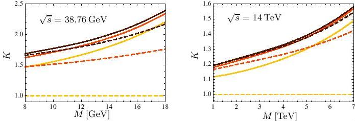
Figure 3: Convergence of the DY $K$-factor at threshold: dashed lines refer to the fixed-order calculation (from bottom to top: LO, NLO, NNLO); solid lines to the corresponding resummed result (taken from [45]).

3 Summary

Soft-collinear effective theory helps: to separate dynamical effects related to different energy-momentum scales appearing in processes involving soft and energetic (but low-virtuality) particles; to establish the corresponding factorization theorems; to define/identify process-independent non-perturbative input parameters/functions; and to resum large logarithms in RG-improved perturbation theory. Among the most important applications in inclusive $B$-decays are the precise determination of $|V_{ub}|$ from $B\to X_{u}\ell\nu$ and SM precision tests in $B\to X_{s}\gamma$ (see section 2.1). Factorization theorems in exclusive decays reduce the non-perturbative input to universal transition form factors and process-independent LCDAs, which can be studied by standard non-perturbative methods (section 2.2). Finally, SCET can be used for systematic studies of radiative corrections in collider processes, like EW Sudakov effects, Drell-Yan production at threshold (section 2.3), and also top-quark jets [16], 4-Fermion Production near $WW$-threshold [47], and traditional QCD applications in jet physics and parton showers [3].

References

-
[1]
M. Neubert,
Phys. Rev. D 49 (1994) 3392.
I. I. Y. Bigi, M. A. Shifman, N. G. Uraltsev and A. I. Vainshtein, Int. J. Mod. Phys. A 9 (1994) 2467. -
[2]
C. W. Bauer, S. Fleming, D. Pirjol and I. W. Stewart,
Phys. Rev. D 63 (2001) 114020.
J. Chay and C. Kim, Phys. Rev. D 65 (2002) 114016.
M. Beneke, A. P. Chapovsky, M. Diehl and Th. Feldmann, Nucl. Phys. B 643 (2002) 431. - [3] For further references see also C. W. Bauer, in these proceedings.
- [4] M. Beneke and Th. Feldmann, Phys. Lett. B 553 (2003) 267.
- [5] C. W. Bauer, S. Fleming and M. E. Luke, Phys. Rev. D 63 (2000) 014006.
- [6] Workshop on Soft-Collinear Effective Theory, Schloss Waldthausen near Mainz (Germany), April 2-5, 2008. [http://wwwthep.physik.uni-mainz.de/scet08/site/]
- [7] G. P. Korchemsky and G. Sterman, Phys. Lett. B 340 (1994) 96.
- [8] R. Akhoury and I. Z. Rothstein, Phys. Rev. D 54 (1996) 2349.
- [9] C. W. Bauer and A. V. Manohar, Phys. Rev. D 70 (2004) 034024.
- [10] S. W. Bosch, B. O. Lange, M. Neubert and G. Paz, Nucl. Phys. B 699 (2004) 335; B. O. Lange, M. Neubert and G. Paz, Phys. Rev. D 72 (2005) 073006.
- [11] K. S. M. Lee, Z. Ligeti, I. W. Stewart and F. J. Tackmann, Phys. Rev. D 74, 011501 (2006); Z. Ligeti, talk presented at [6].
-
[12]
R. Bonciani and A. Ferroglia,
arXiv:0809.4687 [hep-ph].
H. M. Asatrian, C. Greub and B. D. Pecjak, arXiv:0810.0987 [hep-ph].
M. Beneke, T. Huber and X. Q. Li, arXiv:0810.1230 [hep-ph].
G. Bell, arXiv:0810.5695 [hep-ph]. -
[13]
K. Melnikov and A. Mitov,
Phys. Lett. B 620 (2005) 69.
I. R. Blokland et al., Phys. Rev. D 72 (2005) 033014.
H. M. Asatrian et al., Nucl. Phys. B 749 (2006) 325. - [14] T. Becher and M. Neubert, Phys. Lett. B 637 (2006) 251.
- [15] H. Boos, Th. Feldmann, T. Mannel and B. D. Pecjak, JHEP 0605 (2006) 056.
- [16] S. Fleming, A. H. Hoang, S. Mantry and I. W. Stewart, Phys. Rev. D 77 (2008) 114003; A. H. Hoang and A. Jain, talks presented at [6].
- [17] T. Becher and M. Neubert, Phys. Lett. B 633 (2006) 739.
-
[18]
K. S. M. Lee and I. W. Stewart,
Nucl. Phys. B 721, 325 (2005).
S. W. Bosch, M. Neubert and G. Paz, JHEP 0411, 073 (2004).
M. Beneke, F. Campanario, T. Mannel and B. D. Pecjak, JHEP 0506, 071 (2005).
F. J. Tackmann, Phys. Rev. D 72, 034036 (2005). -
[19]
B. O. Lange, M. Neubert and G. Paz,
JHEP 0510, 084 (2005);
B. O. Lange,
JHEP 0601 (2006) 104.
A. K. Leibovich, I. Low and I. Z. Rothstein, Phys. Rev. D 61, 053006 (2000).
A. H. Hoang, Z. Ligeti and M. Luke, Phys. Rev. D 71, 093007 (2005).
K. S. M. Lee, Phys. Rev. D 78 (2008) 013002. - [20] Z. Ligeti, I. W. Stewart and F. J. Tackmann, arXiv:0807.1926 [hep-ph].
- [21] G. Paz, talk presented at [6].
- [22] M. Beneke, G. Buchalla, M. Neubert and C. T. Sachrajda, Phys. Rev. Lett. 83 (1999) 1914; Nucl. Phys. B 606 (2001) 245.
-
[23]
G. P. Korchemsky, D. Pirjol and T. M. Yan,
Phys. Rev. D 61 (2000) 114510.
E. Lunghi, D. Pirjol and D. Wyler, Nucl. Phys. B 649 (2003) 349.
S. W. Bosch, R. J. Hill, B. O. Lange and M. Neubert, Phys. Rev. D 67 (2003) 094014.
S. Descotes-Genon and C. T. Sachrajda, Nucl. Phys. B 650 (2003) 356. - [24] M. Beneke and Th. Feldmann, Nucl. Phys. B 592 (2001) 3.
- [25] M. Beneke and Th. Feldmann, Nucl. Phys. B 685 (2004) 249.
-
[26]
M. Beneke, Th. Feldmann and D. Seidel,
Nucl. Phys. B 612, 25 (2001).
S. W. Bosch and G. Buchalla, Nucl. Phys. B 621 (2002) 459.
A. Ali and A. Y. Parkhomenko, Eur. Phys. J. C 23 (2002) 89. - [27] B. O. Lange and M. Neubert, Nucl. Phys. B 690 (2004) 249 [Erratum-ibid. B 723 (2005) 201]; T. Becher, R. J. Hill and M. Neubert, Phys. Rev. D 72 (2005) 094017.
-
[28]
R. J. Hill and M. Neubert,
Nucl. Phys. B 657, 229 (2003);
T. Becher, R. J. Hill and M. Neubert,
Phys. Rev. D 69, 054017 (2004).
C. W. Bauer, D. Pirjol and I. W. Stewart, Phys. Rev. D 67 (2003) 071502. - [29] G. Bell, Nucl. Phys. B 795 (2008) 1.
-
[30]
M. Beneke and S. Jäger,
Nucl. Phys. B 751 (2006) 160.
N. Kivel, JHEP 0705, 019 (2007).
V. Pilipp, Nucl. Phys. B 794, 154 (2008). - [31] M. Beneke and S. Jäger, Nucl. Phys. B 768, 51 (2007).
- [32] A. Ali, B. D. Pecjak and C. Greub, Eur. Phys. J. C 55, 577 (2008).
- [33] A. G. Grozin and M. Neubert, Phys. Rev. D 55 (1997) 272.
- [34] B. O. Lange and M. Neubert, Phys. Rev. Lett. 91, 102001 (2003).
- [35] V. M. Braun, D. Y. Ivanov and G. P. Korchemsky, Phys. Rev. D 69, 034014 (2004).
- [36] S. J. Lee and M. Neubert, Phys. Rev. D 72, 094028 (2005).
- [37] G. Bell and Th. Feldmann, JHEP 0804, 061 (2008); G. Bell, talk presented at [6].
- [38] P. Ball, V. M. Braun and E. Gardi, Phys. Lett. B 665, 197 (2008).
-
[39]
A. V. Efremov and A. V. Radyushkin,
Phys. Lett. B 94, 245 (1980).
G. P. Lepage and S. J. Brodsky, Phys. Lett. B 87, 359 (1979). - [40] F. De Fazio, Th. Feldmann and T. Hurth, Nucl. Phys. B 733, 1 (2006) [Erratum-ibid. B 800, 405 (2008)]; JHEP 0802, 031 (2008); F. De Fazio, talk presented at [6].
- [41] A. Khodjamirian, T. Mannel and N. Offen, Phys. Lett. B 620 (2005) 52.
-
[42]
P. Ciafaloni and D. Comelli,
Phys. Lett. B 446 (1999) 278.
V. S. Fadin, L. N. Lipatov, A. D. Martin and M. Melles, Phys. Rev. D 61 (2000) 094002.
J. H. Kühn, A. A. Penin and V. A. Smirnov, Eur. Phys. J. C 17 (2000) 97.
- [43] J. y. Chiu, F. Golf, R. Kelley and A. V. Manohar, Phys. Rev. Lett. 100 (2008) 021802; A. V. Manohar and J. y. Chiu, talks presented at [6].
- [44] J. y. Chiu, F. Golf, R. Kelley and A. V. Manohar, Phys. Rev. D 77 (2008) 053004.
- [45] T. Becher, M. Neubert and G. Xu, JHEP 0807 (2008) 030; T. Becher and V. Ahrens talks at [6].
- [46] A. Idilbi and X. d. Ji, Phys. Rev. D 72, 054016 (2005).
- [47] M. Beneke, P. Falgari, C. Schwinn, A. Signer and G. Zanderighi, Nucl. Phys. B 792, 89 (2008); G. Zanderighi, talk presented at [6].