Braneworlds with timelike extra-dimension

Abstract

In this work, we consider a braneworld model with a timelike extra-dimension. There are strong constraints to the parameter values of such a model resulting from the claim that there must be a physical solution to the Friedmann equation at least between now and the time of recombination. We fitted the model to supernova type Ia data and checked the consistency of the result with other observations. For parameter values that are consistent with observations, the braneworld model is indistinguishable from a $\Lambda$CDM universe as far as the considered cosmological tests are concerned.

I Introduction

After the seminal papers of Randall and Sundrum Randall and Sundrum (1999a, b) several braneworld models have been examined during the past years (for reviews see Maartens (2004); Koyama (2008)). The idea is that we could be living in a four-dimensional space-time, the brane, which is embedded in or bounding a five-dimensional bulk. Gravity acts in all five dimensions whereas the other interaction forces are constrained to the brane. Thus, the existence of an additional dimension influences the expansion history of the universe. While the Randall-Sundrum model differs from general relativity in the early universe, another braneworld model was suggested by Dvali, Gabadadze and Porrati (DGP model) Dvali et al. (2000) which differs from general relativity at late times and thus could give an explanation for the present accelerated expansion. In fact, braneworld cosmologies (e.g. a combination of the Randall-Sundrum and the DGP model Collins and Holdom (2000); Sahni and Shtanov (2002)) can mimick several other cosmological models, but also allow for a variety of other expansion histories Sahni (2005). In most models the extra-dimension is considered to be spacelike, but there is actually no a priori reason that prevents this dimension from being timelike.

In the present work we consider a model with a single brane which forms the boundary of the bulk. Chapter II summarizes the most important properties of this model that has already been described by Shtanov and Sahni Shtanov and Sahni (2003); Shtanov (2002). Here, we take a look at the general case, leaving open the nature of the fifth dimension. In capter III we draw our attention to the case of a timelike extra-dimension. We put new constraints on the density parameters in order to get a physical solution of the Friedmann equation within a certain redshift range. At this point, the so-called BRANE2 model can already be excluded in the case of vanishing spatial curvature and dark radiation. The BRANE1 model is then confronted with observational data showing that it cannot be excluded by the applied cosmological tests.

II A Braneworld Model

We consider a theory which combines the Randall-Sundrum and the DGP model and is described by the action Shtanov and Sahni (2003); Shtanov (2002)

$$S = M^{3}\left[\int_{\mbox{\footnotesize bulk}}(\mathcal{R}-2\Lambda_{5})\sqrt{-\epsilon g}\,d^{5}x\right.$$ (1)

$$\qquad\left.-2\epsilon\int_{\mbox{\footnotesize brane}}K\sqrt{-h}\,d^{4}x\right]$$

$${}+\int_{\mbox{\footnotesize brane}}(m^{2}R-2\sigma)\sqrt{-h}\,d^{4}x$$

$${}+\int_{\mbox{\footnotesize brane}}L(h_{ab},\phi)\sqrt{-h}\,d^{4}x\,,$$

where $M$ and $m$ are the five- and four-dimensional Planck masses, respectively. The two masses are related by an important length scale $\ell=2m^{2}/M^{3}$. On short length scales $(r\ll\ell)$ the usual four-dimensional general relativity is recovered, while on large length scales $(r\gg\ell)$ five-dimensional effects play an important role Sahni and Shtanov (2003); Dvali et al. (2000). $\mathcal{R}$ denotes the scalar curvature of the bulk metric $g_{ab}$ and $R$ the scalar curvature of the induced brane metric $h_{ab}=g_{ab}-\epsilon n_{a}n_{b}$, with $n^{a}$ being the inner unit normal vector field to the brane. $K$ is the trace of the extrinsic curvature of the brane $K_{ab}=h^{c}_{\,\,a}\nabla_{c}n_{b}$. $\Lambda_{5}$ denotes the bulk cosmological constant and $\sigma$ the brane tension. As ordinary matter fields are confined to the brane, the Lagrangian density $L$ does not depend on the bulk metric $g_{ab}$, but on the induced metric $h_{ab}$. For a spacelike extra-dimension $\epsilon=1$, whereas $\epsilon=-1$ for a timelike extra-dimension.

By variation of this action one obtains Einstein’s equations in the bulk

$$\mathcal{G}_{ab}+\Lambda_{5}g_{ab}=0$$ (2)

and on the brane

$$m^{2}G_{ab}+\sigma h_{ab}=T_{ab}+\epsilon M^{3}(K_{ab}-Kh_{ab})\,.$$ (3)

In order to calculate the five-dimensional Friedmann equations from the above Einstein equations one needs the Gauss-Codacci-relation (Wald (1984) chapter 10.2):

$$R_{abc}^{\quad\;d}=h_{a}^{\;\;f}h_{b}^{\;\;g}h_{c}^{\;\;k}h^{d}_{\;\;j}\mathcal{R}_{fgk}^{\quad\;j}+K_{ac}K_{b}^{\;\;d}-K_{bc}K_{a}^{\;\;d}$$ (4)

Contracting this relation on the brane leads to

$$M^{6}\left(R-2\Lambda_{5}\right)- \frac{1}{3}\left(m^{2}R-4m^{2}\Lambda_{4}+T\right)^{2}$$

$${}+ \left(m^{2}G_{ab}+m^{2}\Lambda_{4}h_{ab}-T_{ab}\right)$$

$$\times\left(m^{2}G^{ab}+m^{2}\Lambda_{4}h^{ab}-T^{ab}\right)=0$$ (5)

In the following, we consider a homogeneous and isotropic universe. Taking the stress energy conservation into account, the above equation can be integrated to yield Shtanov (2002); Deffayet (2001)

$$m^{4}\left(H^{2}+\frac{k}{a^{2}}-\frac{\rho+\sigma}{3m^{2}}\right)^{2}$$

$$=\epsilon M^{6}\left(H^{2}+\frac{k}{a^{2}}-\frac{\Lambda_{5}}{6}-\frac{C}{a^{4}}\right)\,,$$ (6)

where $H=\dot{a}/a$ is the Hubble parameter and $k=0,\pm 1$ corresponds to the spatial curvature. $\rho$ is the matter density on the brane. $C$ is an integration constant, the dark radiation term, which transmits bulk graviton influence onto the brane. Introducing the length scale $\ell=2m^{2}/M^{3}$ equation (II) yields the Friedmann equation on the brane

$$H^{2}+\frac{k}{a^{2}}$$ (8)

$$= \frac{\rho+\sigma}{3m^{2}}$$

$${}+\epsilon\frac{2}{\ell^{2}}\left[1\pm\sqrt{1+\epsilon\ell^{2}\left(\frac{\rho+\sigma}{3m^{2}}-\frac{\Lambda_{5}}{6}-\frac{C}{a^{4}}\right)}\right]$$

$$= \frac{\Lambda_{5}}{6}+\frac{C}{a^{4}}$$

$$+\epsilon\frac{1}{\ell^{2}}\left[1\pm\sqrt{1+\epsilon\ell^{2}\left(\frac{\rho+\sigma}{3m^{2}}-\frac{\Lambda_{5}}{6}-\frac{C}{a^{4}}\right)}\right]^{2}\,.$$

The $\pm$-sign corresponds to the two different ways the brane can be embedded in the bulk. The model which is described by the equation with the lower sign will from now on be referred to as BRANE1 and the one with the upper sign as BRANE2.

Using the cosmological density parameters

$$\Omega_{m} =\frac{\rho_{0}}{3m^{2}H_{0}^{2}},\quad \Omega_{k} =-\frac{k}{a_{0}^{2}H_{0}^{2}},\quad \Omega_{\sigma} =\frac{\sigma}{3m^{2}H_{0}^{2}}$$

$$\Omega_{\ell} =\frac{1}{\ell^{2}H_{0}^{2}}, \Omega_{\Lambda_{5}} =-\frac{\Lambda_{5}}{6H_{0}^{2}}, \Omega_{C} =-\frac{C}{a_{0}^{4}H_{0}^{2}}$$

the Friedmann equation can be rewritten as

$$\frac{H^{2}(z)}{H_{0}^{2}}=\Omega_{m}(1+z)^{3}+\Omega_{k}(1+z)^{2}+\Omega_{\sigma}$$

$${}+2\epsilon\Omega_{\ell}{}\pm 2\epsilon\sqrt{\Omega_{\ell}}$$

$$\times\sqrt{\Omega_{\ell}+\epsilon\left[\Omega_{m}(1+z)^{3}+\Omega_{\sigma}+\Omega_{\Lambda_{5}}+\Omega_{C}(1+z)^{4}\right]}\,.$$ (9)

Considering only the first three terms on the RHS, we receive the well-known Friedmann equation of four-dimensional general relativity. This is equivalent to setting the five-dimensional Planck mass $M$ to zero (i.e. $\Omega_{\ell}=0$). If we instead (in the case of a spacelike extra-dimension) choose the four-dimensional Planck mass $m$ to be zero, the result is a Randall-Sundrum braneworld model Randall and Sundrum (1999a, b).

In the approach we follow in this work, there is no need to specify a metric. The Friedmann equation could be derived without making any assumptions on the metric except homogeneity and isotropy. This makes the ansatz rather general. Nevertheless, we give an example for a metric. In the case $m=0$, the bulk can be described by the following metric Shtanov and Sahni (2003):

$$ds^{2}=-f(r)dt^{2}+\frac{\epsilon dr^{2}}{f(r)}+r^{2}d\Omega_{3}\;,$$ (10)

where

$$f(r)=\epsilon\left(k-\frac{\Lambda_{5}r^{2}}{6}-\frac{C}{r^{2}}\right)$$ (11)

and $d\Omega_{3}$ denotes the metric of the unit three-sphere. For a spacelike extra-dimension, this solution corresponds to AdS₅-Schwarzschild.

III Timelike Extra-dimension

We will now focus on the case of a timelike extra-dimension. Thus, the Friedmann equation is

$$\frac{H^{2}(z)}{H_{0}^{2}}=\Omega_{m}(1+z)^{3}+\Omega_{k}(1+z)^{2}+\Omega_{\sigma}$$

$${}-2\Omega_{\ell}{}\mp 2\sqrt{\Omega_{\ell}}$$

$$\times\sqrt{\Omega_{\ell}-\Omega_{m}(1+z)^{3}-\Omega_{\sigma}-\Omega_{\Lambda_{5}}-\Omega_{C}(1+z)^{4}}\,.$$ (12)

From equation (8) the following constraint on the density parameters can be obtained by setting $z=0$:

$$1 = \Omega_{k}-\Omega_{\Lambda_{5}}-\Omega_{C}$$ (13)

$${}-\left[\sqrt{\Omega_{\ell}}\pm\sqrt{\Omega_{\ell}-\Omega_{m}-\Omega_{\sigma}-\Omega_{\Lambda_{5}}-\Omega_{C}}\right]^{2}$$

As the density parameters are real quantities,

$$\Omega_{\ell}\geq 0,$$ (14)

$$\Omega_{\ell}\geq\Omega_{m}+\Omega_{\sigma}+\Omega_{\Lambda_{5}}+\Omega_{C}$$ (15)

as well as

$$\Omega_{k}-\Omega_{\Lambda_{5}}-\Omega_{C}\geq 1$$ (16)

must be fulfilled. For a $\Lambda$CDM universe, we know from observations that the spatial curvature $\Omega_{k}$ is close to zero. Komatsu et al. Komatsu et al. (2008) have constrained the spatial curvature to be $\Omega_{k}=-0.0052\pm 0.0064$ by using WMAP5 data. On the other hand, the dark radiation density at the present epoch $\Omega_{C}$ also has to be quite small as it scales with $(1+z)^{4}$. Assuming that the constraints on the spatial curvature are also valid for braneworld models, from the above equation follows $\Omega_{\Lambda_{5}}\lesssim-1$. At least $\Omega_{\Lambda_{5}}$ has to be negative, i.e. the bulk cosmological constant $\Lambda_{5}$ is positive.

III.1 Vanishing Dark Radiation and Spatial Curvature

For simplicity we first consider a model with $\Omega_{k}=0=\Omega_{C}$. In this case, the only parameter that scales with redshift is the matter density. As the BRANE1 and the BRANE2 models show quite a different behaviour, we discuss them separately.

III.1.1 BRANE1

Two conditions have to be satisfied in (12): $H^{2}(z)$ (condition 1) as well as the term under the square root (condition 2) must not be negative.
Condition 1:

$$\Omega_{m}(1+z)^{3}+\Omega_{\sigma}-2\Omega_{\ell}$$

$${}+2\sqrt{\Omega_{\ell}}\sqrt{\Omega_{\ell}-\Omega_{m}(1+z)^{3}-\Omega_{\sigma}-\Omega_{\Lambda_{5}}} \geq 0$$ (17)

Condition 2:

$$\Omega_{m}(1+z)^{3}\leq\Omega_{\ell}-\Omega_{\Lambda_{5}}-\Omega_{\sigma}\,.$$ (18)

From the constraint equation (13) we receive two solutions for the brane tension

$$\Omega_{\sigma}=1-\Omega_{m}\pm 2\sqrt{\Omega_{\ell}}\sqrt{-1-\Omega_{\Lambda_{5}}}\,.$$ (19)

The constraints on the density parameters given by condition 1 and 2 strongly depend on whether a negative or positive brane tension is chosen.

In the case of a negative $\Omega_{\sigma}$, either the inequality

$$\Omega_{\ell}\geq\left(\frac{\Omega_{m}(1+z)^{3}+1-\Omega_{m}}{2\left(\sqrt{-\Omega_{\Lambda_{5}}}+\sqrt{-\Omega_{\Lambda_{5}}-1}\right)}\right)^{2}$$ (20)

or the inequalities

$$\sqrt{\Omega_{\ell}} \geq \sqrt{\Omega_{m}(1+z)^{3}-\Omega_{m}}-\sqrt{-1-\Omega_{\Lambda_{5}}}\quad\text{and}$$

$$\Omega_{\ell} \leq -\Omega_{\Lambda_{5}}$$ (21)

have to be fulfilled.

For a positive $\Omega_{\sigma}$,

$$\Omega_{\ell}\geq\left(\frac{\Omega_{m}(1+z)^{3}+1-\Omega_{m}}{2\left(\sqrt{-\Omega_{\Lambda_{5}}}-\sqrt{-\Omega_{\Lambda_{5}}-1}\right)}\right)^{2}$$ (22)

must be fulfilled.

From the constraint inequalities one can immediately see that there exists a maximum redshift beyond which the Friedmann equation does not have a physical solution. We claim that the conditions must at least be satisfied back to the time of recombination, i.e. $z=1090$. When going to higher redshifts, at some point either (III.1.1) or (18) is violated. The physical meaning of the former case is the following: In a collapsing universe the Hubble parameter $H(z)$ becomes zero at a certain redshift and a bounce takes place Shtanov and Sahni (2003). After that the universe expands again. In contrast, violation of (18) would lead to a singularity similar to those described in Shtanov and Sahni (2002): The deceleration parameter $q(z)=-\ddot{a}/(aH^{2})$ becomes singular whereas $H(z)$ remains finite.

The conditions that constrain the density parameters in the cases of negative and positive brane tension are quite similar. Yet, the consequences for the allowed parameter space are very different as can be seen in Figs. 1 and 2. The range of possible parameter values is much larger for a negative brane tension. Therefore, we will focus on this case in the following.

Figure 1: Constraints on the density parameters $\Omega_{\ell}$ and $\Omega_{\Lambda_{5}}$ of a BRANE1 model with negative brane tension and $\Omega_{m}=0.3$.

Figure 2: Constraints on the density parameters $\Omega_{\ell}$ and $\Omega_{\Lambda_{5}}$ of a BRANE1 model with positive brane tension and $\Omega_{m}=0.3$.

Figure 3 shows how the square of the Hubble parameter changes with increasing $\Omega_{\ell}$, while $\Omega_{m}=0.3$ and $\Omega_{\Lambda_{5}}=-2$ stay fixed for the case of a negative brane tension. For values of $\Omega_{\ell}$ smaller than $\sim 10^{16}$ (i.e. values within the excluded parameter range), the curve becomes negative between now and the time of recombination. In Fig. 4, it is shown how the curve changes when $\Omega_{\Lambda_{5}}$ is varied. Here, all parameter values are in the allowed range. With increasing $\Omega_{\Lambda_{5}}$ the curves become steeper and thus approach the $\Lambda$CDM model (which cannot be shown in this figure as it is too steep).

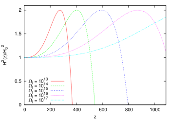
Figure 3: Hubble parameter $H^{2}(z)/H^{2}_{0}$ of a BRANE1 model with negative brane tension for different values of $\Omega_{\ell}$ with $\Omega_{m}=0.3$ and $\Omega_{\Lambda_{5}}=-2$.

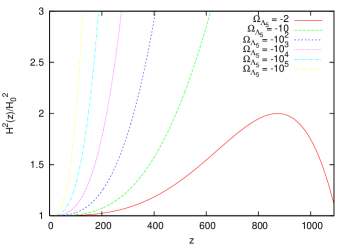
Figure 4: Hubble parameter $H^{2}(z)/H^{2}_{0}$ of a BRANE1 model with negative brane tension for different values of $\Omega_{\Lambda_{5}}$ with $\Omega_{m}=0.3$ and $\Omega_{\ell}=10^{16}$.

III.1.2 BRANE2

For the BRANE2 model again two conditions have to be fulfilled:

$$\Omega_{m}(1+z)^{3}+\Omega_{\sigma}-2\Omega_{\ell}$$

$${}-2\sqrt{\Omega_{\ell}}\sqrt{\Omega_{\ell}-\Omega_{m}(1+z)^{3}-\Omega_{\sigma}-\Omega_{\Lambda_{5}}} \geq 0$$ (23)

and

$$\Omega_{\ell}-\Omega_{m}(1+z)^{3}-\Omega_{\sigma}-\Omega_{\Lambda_{5}}\geq 0\,,$$ (24)

where the brane tension is given by $\Omega_{\sigma}=1-\Omega_{m}+2\sqrt{\Omega_{\ell}}\sqrt{-1-\Omega_{\Lambda_{5}}}$.

These conditions are equivalent to the inequalities

$$\Omega_{\ell}\leq\frac{1}{4(\sqrt{-\Omega_{\Lambda_{5}}}-\sqrt{-1-\Omega_{\Lambda_{5}}})^{2}}$$ (25)

and

$$\Omega_{\ell}\geq(\sqrt{\Omega_{m}(1+z)^{3}-\Omega_{m}}+\sqrt{-1-\Omega_{\Lambda_{5}}})^{2}\,.$$ (26)

The two inequalities can only be fulfilled simultaneously, if the RHS of (25) is larger than the RHS of (26). This is only possible for redshifts $z\lesssim 0.22$. Thus, a flat BRANE2 model without dark radiation can be excluded.

III.1.3 Angular Separation

In the following we will concentrate on the BRANE1 model with negative brane tension. Remember that in this section we consider the universe to be spatially flat and to contain no dark radiation. We would now like to know whether such a model is compatible with observations. One simple cosmological test is to take a look at the angular separation. The angle $\Theta(z)$ under which we see two objects in the universe depends on the cosmological model. As the universe expands, the distance $D(z)$ between those objects changes as

$$D(z)=\frac{D_{0}}{1+z}\,,$$ (27)

where $D_{0}=D(z=0)$ is the separation in the present universe. The angular separation is described by

$$\Theta(z) = \frac{D(z)(1+z)^{2}}{d_{L}(z)}=\frac{D_{0}(1+z)}{d_{L}(z)}$$ (28)

$$= D_{0}\left[\int_{0}^{z}\frac{dz^{\prime}}{H(z^{\prime})}\right]^{-1}\,,$$

where $d_{L}(z)$ is the luminosity distance and the last equation is only valid for a flat universe, $\Omega_{k}=0$.

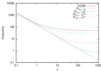
Figure 5: Angular separation for a $\Lambda$CDM ($\Omega_{m}=0.3$, $\Omega_{\Lambda}=0.7$) and a BRANE1 model for different values of $\Omega_{\Lambda_{5}}$ with $\Omega_{m}=0.3$, $\Omega_{\ell}=10^{16}$ and $D_{0}=185$Mpc.

The large-scale correlation function of luminous red galaxies has been obtained from Sloan Digital Sky Survey data showing a peak at 100 $h^{-1}$ Mpc Eisenstein et al. (2005). The average redshift of those galaxies is $z=0.35$. Assuming $h=0.73$, we can determine the present separation to be $D_{0}=185$ Mpc. If one uses this typical distance of large objects in the present universe and calculates $\Theta$ for $z=1090$ with the above formula, the resulting angle should be a typical value for the structure observed in the CMB. Figure 5 shows the angular separation for $\Lambda$CDM and for BRANE1. $\Theta(z=1090)=48.5$arcmin in a $\Lambda$CDM universe, which is where the first peak of the CMB power spectrum is located. Thus, $\Lambda$CDM fits the observational data perfectly well. For small absolute values of $\Omega_{\Lambda_{5}}$ in the braneworld model, the angular width $\Theta(z=1090)$ is about 300 times smaller than in the $\Lambda$CDM case and thus not compatible with CMB observations. This cannot be remedied by changing the value of $\Omega_{\ell}$. The larger $\Omega_{\Lambda_{5}}$ is chosen the more the angular width approaches that of $\Lambda$CDM. Therefore a small $\Omega_{\Lambda_{5}}$ can be ruled out for this special kind of braneworld model with $\Omega_{k}=0$ and $\Omega_{C}=0$.

III.2 BRANE1 with Dark Radiation and Spatial Curvature

In this section we give up the assumption of a flat universe without dark radiation. Instead we assume a negative $\Omega_{C}$, which corresponds to a positive dark radiation term $C$. $\Omega_{k}$ can have arbitrary values.

Figure 6: $H(z)/H_{\Lambda\mbox{\footnotesize CDM}}(z)$ for a BRANE1 closed universe with dark radiation. $\Omega_{m}=0.3$ and $\Omega_{k}=-0.01$ for all curves, $\Omega_{\Lambda_{5}}=-2$ and $\Omega_{\ell}=10^{16}$ for the lower three bold lines and $\Omega_{\Lambda_{5}}=-10^{8}$ and $\Omega_{\ell}=10^{8}$ for the upper three lines.

Figure 6 shows $H(z)/H_{\Lambda\mbox{\footnotesize CDM}}(z)$ for different parameter values. Without dark energy (and with small $\Omega_{\Lambda_{5}}$) there was a large difference between the braneworld model and $\Lambda$CDM. $H^{2}(z)$ became even negative at a certain redshift. Models including dark radiation only deviate from the standard model at relatively low redshifts. The largest deviations occur around redshift $\simeq 1$. With increasing $z$ the Hubble parameter approaches that of the $\Lambda$CDM case.

A good method to compare the predictions for those redshifts with observations is to consider the luminosity distance $d_{L}(z)$ or the distance modulus $\mu(z)$. The luminosity distance is given by

$$d_{L}(z)=\frac{1+z}{H_{0}\sqrt{|\Omega_{k}|}}\,\mathcal{S}\left(\sqrt{|\Omega_{k}|}\int_{0}^{z}\frac{H_{0}\,dz^{\prime}}{H(z^{\prime})}\right)\,,$$ (29)

where $\mathcal{S}(x)=x$ for a flat, $\sin(x)$ for a closed and $\sinh(x)$ for an open universe. The distance modulus is defined as

$$\mu(z)=m(z)-M=5\log d_{L}(z)+25\,,$$ (30)

where $d_{L}$ is given in units of Mpc. $m(z)$ and $M$ are the apparent and the absolute magnitude, respectively. The observational data are obtained by analyzing supernovae type Ia as they are considered to be the best standard candles.

We used the 2007 Gold sample presented by Riess et al. Riess et al. (2007) to fit the model. We adopted the values of $M$ and $H_{0}$ given by Riess et al. (2005). Therefore, we had to substract 0.27mag from distance modulus given in the Gold sample. Then the value of $H_{0}$ is 73km/(s Mpc). The problem with the $\chi^{2}$-fit is that there exist multiple local minima for $\chi^{2}$ with many of those minima having the same value of $\chi^{2}$. As shown in Fig. 3, for some parameter values $H^{2}(z)$ becomes zero before $z=1090$ is reached. Fits that yielded such values could be dismissed at once. Fitting all five parameters ($\Omega_{m}$, $\Omega_{\ell}$, $\Omega_{\Lambda_{5}}$, $\Omega_{C}$ and $\Omega_{k}$), the results for $\Omega_{k}$ were always negative and typically between $-0.2$ and $-0.6$. An example of best fit parameters is given in table 1. If we accept the results from the WMAP observation (that were obtained by assuming $\Lambda$CDM) to be valid also for braneworld models, then the result of our fit is not compatible with WMAP which predicts a flat universe Komatsu et al. (2008). Also the calculated value for $\Omega_{C}$ is quite surprising. As the dark radiation density scales with $(1+z)^{4}$, it should be close to zero at the present epoch. So if the value $-1.15$ is correct, $\Omega_{C}$ must have been extremely large at earlier times. Yet, it is noticeable that the braneworld model with a $\chi^{2}$ per degree of freedom of 0.89 fits the supernova data slightly better than $\Lambda$CDM with a $\chi^{2}$ per degree of freedom of 0.90.

	$\Omega_{m}$	$\Omega_{\ell}$	$\Omega_{\Lambda_{5}}$	$\Omega_{C}$		$\Omega_{k}$		$\chi^{2}_{\mbox{\scriptsize dof}}$
5-parameter	0.38	$1.9\cdot 10^{14}$	$-7.8\cdot 10^{16}$	$-1$	$.15$	$-0$	$.45$	0.89
4-parameter	0.27	$1.7\cdot 10^{15}$	$-6.0\cdot 10^{13}$	$-0$	$.17$	$0$		0.89
3-parameter	0.31	$2.0\cdot 10^{14}$	$-1.5\cdot 10^{16}$	0		$0$		0.91
$\Lambda$CDM	0.28		$\Omega_{\Lambda}=0.72$					0.90

Table 1: Results of the $\chi^{2}$-fits for 3-, 4- and 5-parameter fits of the BRANE1 model and for $\Lambda$CDM.

We fixed $\Omega_{k}$ to be equal to zero and performed a 4-parameter fit. The $\chi^{2}$ per degree of freedom for that fit is 0.89. This is the same value as for the 5-parameter fit. The absolute value of $\Omega_{C}$ has become smaller compared to the previous fit. But still it seems to be quite large. Performing another fit with $\Omega_{C}$ and $\Omega_{k}$ fixed to zero yields a $\chi^{2}$ per degree of freedom of 0.91, which is slightly worse than that of $\Lambda$CDM. The density parameters have reasonable values.

Figure 7 shows the distance modulus for the three fits and the $\Lambda$CDM fit compared to the Gold sample. In Fig. 8 the angular separation of the same models is plotted. In both plots the curve of the 3-parameter fit is almost identical to that of $\Lambda$CDM. While the 4- and 5-parameter fits are perfectly consistent with SNe observations, the calculated angular separations at redshift 1090 are too large to be compatible with CMB observations, namely $\Theta\simeq 80$ arcmin for the 4-parameter fit and $\Theta\simeq 100$ arcmin for the 5-parameter fit. Thus, the results obtained by those two fits to SN data can be ruled out and we are left with the result of the 3-parameter fit. This model almost does not differ from $\Lambda$CDM as far as the distance modulus and the angular separation are concerned and thus both theories are indistinguishable when using only the two applied test.

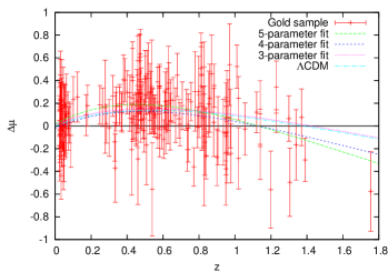
Figure 7: Distance modulus minus the distance modulus of an empty universe for the three braneworld model fits and $\Lambda$CDM.

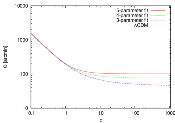
Figure 8: Angular separation for the three braneworld model fits and $\Lambda$CDM.

Table 2 lists the following quantities for the three fits: a) the angular separation $\Theta$ at the time recombination, b) the maximum possible redshift $z_{\text{max}}$ for which the Friedmann equation has a physical solution and c) the age of the universe. For the calculation of the maximum redshift and the age of the universe, one needs to consider the radiation density $\Omega_{r}$ in the Friedmann equation, which could be neglected in the previous tests, but becomes important at very high redshifts. In order to do so, we just need to add $\Omega_{r}(1+z)^{4}$ to $\Omega_{m}(1+z)^{3}$ every time it occurs in the Friedmann equation. We adopt the value $\Omega_{r}=8.4\cdot 10^{-5}$ according to WMAP5 Komatsu et al. (2008). The redshift is only limited for the 3-parameter fit, where the term under the square root in the Friedmann equation (12) becomes zero at $z_{\text{max}}$. At this point a singularity occurs, which can be interpreted as a kind of Big Bang.

	$\Theta$[arcmin]	$z_{\text{max}}$	age [Gyr]
5-parameter fit	104	$\infty$	10.4
4-parameter fit	77	$\infty$	12.9
3-parameter fit	46	120000	15.0

Table 2: Angular separation $\Theta$ at recombination, maximum redshift $z_{\text{max}}$ and age of the universe for the different fits.

Let us take a closer look at the result of the 3-parameter fit since this is the only model that has not been excluded by the tests used in this work. In this model, the universe would be 15 billion years old, i.e. there is no conflict with the oldest objects in the universe. It has already been pointed out in Sahni and Shtanov (2003) that the usual four dimensional general relativity is recovered on scales much smaller than $\ell$. Taking the fit result $\Omega_{\ell}=2\cdot 10^{14}$ and assuming $H_{0}=73$ km/(s Mpc), one obtains $\ell\simeq 300$ pc. Thus, the model is not in conflict with any tests of general relativity on scales much smaller than 300 pc. Especially tests that are made within the solar system are not affected by any five-dimensional effects.

A problem occurs when we consider Big Bang nucleosynthesis (BBN). The maximum redshift of the 3-parameter fit is much smaller than the redshift when nucleosynthesis took place. This problem can, however, be easily avoided by introducing again a dark radiation term $\Omega_{C}$. Its value must be small enough to ensure that the fit result and the cosmological tests up to the redshift of recombination are not affected. On the other hand, $\Omega_{C}$ needs to be larger than the radiation density $\Omega_{r}$ to prevent the term under the square root of the Friedmann equation from becoming negative. Thus, we choose $\Omega_{r}$ to be of order $10^{-4}$. Then the model is radiation dominated at very high redshifts, just like the $\Lambda$CDM model. There is no limit to the redshift any more and the model is consistent with BBN observations as it does not differ from $\Lambda$CDM at these redshifts. Thus, this model cannot be excluded by the considered observations.

Remember that these results are only examples as the $\chi^{2}$-fit yields many minima. However, we did not find a result of the 5- or 4-parameter fit that is compatible with all observations.

IV Conclusion

In this work we focused on braneworld models with a timelike extra-dimension. For a flat universe without dark radiation we put constraints on the density parameters $\Omega_{\Lambda_{5}}$ and $\Omega_{\ell}$. The BRANE2 model could be excluded for this case. Considering a BRANE1 model, the absolute value of at least one of the parameters $\Omega_{\Lambda_{5}}$, $\Omega_{\ell}$ has to be very large in order to obtain a physical solution for the Friedmann equation within a redshift range from 0 to 1090. Comparison to CMB data shows that a large $|\Omega_{\Lambda_{5}}|$ is necessary for this model.

We then introduced a dark radiation term and spatial curvature and fitted the density parameters to SN Ia data. The results of the 5- and 4-parameter fits are not compatible with CMB observations. The only result that could not be ruled out is the 3-parameter fit, provided a small dark radiation term is present. Unfortunately, its behaviour in the considered cosmological tests is almost identical to that of $\Lambda$CDM. So, better observational data would not help excluding or confirming the model. Instead, further cosmological tests are needed.