Lattice Gluon Propagator in the Landau Gauge: A Study Using Anisotropic Lattices

Abstract

Lattice gluon propagators are studied using tadpole and Symanzik improved gauge action in Landau gauge. The study is performed using anisotropic lattices with asymmetric volumes. The Landau gauge dressing function for the gluon propagator measured on the lattice is fitted according to a leading power behavior: $Z(q^{2})\simeq(q^{2})^{2\kappa}$ with an exponent $\kappa$ at small momenta. The gluon propagators are also fitted using other models and the results are compared. Our result is compatible with a finite gluon propagator at zero momentum in Landau gauge.

I Introduce and Motivation

Quantum Chromodynamics (QCD) is believed to be fundamental theory for strong interactions in Nature. Almost all information about a quantum field theory is encoded in the Green’s functions and the knowledge of QCD Green’s function is important for the understanding of some of the novel properties of QCD like confinement and asymptotic freedom. Gluon propagators have been studied by various means in the literature. The ultraviolet(UV) behavior of the gluon propagator can be investigated with perturbation theory. In the infra-red (IR) region, however, it has to be treated with non-perturbative methods. One can follow the continuum approaches: such as truncated Dyson-Schwinger equations(DSEs) DSE_intro , exact renormalization group equations RGE_intro , the Fokker-Planck type diffusion equation of stochastic quantization SQ_intro , or the lattice QCD approaches MC_intro1 ; MC_intro2 ; MC_intro3 ; MC_intro4 ; MC_intro5 ; MC_intro6 ; MC_intro7 ; MC_intro8 ; ref1 ; ref2 ; ref3 . The results from these two approaches were also compared. Some agreement were found, however, some important issues remain to be clarified. In this paper, we study the lattice gluon propagator using tadpole improved lattice actions on anisotropic lattices. While most of the previous lattice studies were performed on isotropic lattices, our results can be compared with both the previous lattice results and the results using continuum approaches.

In the study of the IR region of the gluon propagator with lattice QCD, lattice volumes have to be large enough since the minimal momenta is inverse proportion to the spatial dimensions of the lattice. Investigations with different lattices imply apparent finite volume effects finite_vol_eff , and even the extremely asymmetrical box is not safe asym_vol_eff . A lattice with large extensions in all four dimensions will require substantial computational resources. One way to proceed is to adopt a larger lattice spacing. Previous studies on coarse lattices suggest that the lattice spacing error is still under control if an improved lattice action is used spacing_eff . We adopt the tadpole improved gauge action on anisotropic lattices symanzik1 ; symanzik2 ; symanzik3 ; tadpole , which has the advantage of less lattice spacing error and can be used to generate coarser but larger lattice to reach the deeper IR region. We also choose to use anisotropic and asymmetrical lattices to further depress spacing errors and to obtain more low momentum modes.

The anisotropic lattice is a lattice with different cell spacings on different axes. We set the equal spatial spacing $a_{i}=a_{s}$ while the temporal spacing is $a_{t}=\frac{1}{\xi_{0}}a_{s}$ with the anisotropic ratio $\xi_{0}=5$. The anisotropic lattice has the advantage of further reducing the spacing error while the drawback of further breaking the four-dimensional Euclidean symmetry. Therefore, the renormalization effect of anisotropic momenta should be taken into account which introduces an additional parameter to measure and complicates the determination of the physical scale.

II Lattice Formulations

II.1 Gauge Action

We use the tadpole improved gauge action on anisotropic lattices:

$$S=-\beta\sum_{i>j}(\frac{5}{9}\frac{TrP_{ij}}{\xi_{0}u_{s}^{4}}-\frac{1}{36}\frac{TrR_{ij}}{\xi_{0}u_{s}^{6}}-\frac{1}{36}\frac{TrR_{ji}}{\xi_{0}u_{s}^{6}})-\beta\sum_{i}{(\frac{4}{9}\frac{\xi_{0}TrP_{0i}}{u_{s}^{2}}-\frac{1}{36}\frac{\xi_{0}TrR_{i0}}{u_{s}^{4}})}$$ (1)

where $P_{ij}$ is the usual plaquette variable and $R_{ij}$ is the $2\times 1$ spatial Wilson loop on the lattice. The parameter $u_{s}$, which we take to be the forth root of the average spatial plaquette value, incorporates the usual tadpole improvement. The parameter $\xi_{0}$ designates the bare anisotropy.

II.2 Gauge Fixing

The gluon field $\{A_{\mu}(x)\}$ associated with a gauge configuration $\{U_{\mu}(x)\}$ is given by

$$A_{\mu}(x+a_{\mu}\hat{e}_{\mu}/2)=\frac{1}{2ig_{0}}[U_{\mu}(x)-U_{\mu}^{\dagger}(x)]-\frac{1}{6ig_{0}}Tr[U_{\mu}(x)-U_{\mu}^{\dagger}(x)]$$ (2)

We fix the gluon field to Landau gauge

$$\partial_{\mu}A_{\mu}=0$$ (3)

To realize the gauge fix, we first define the gauge transform

$$U_{\mu}^{G}(x)=G(x)U_{\mu}(x)G(x+\hat{\mu})^{\dagger}$$ (4)

where

$$G(x)=e^{-i\sum\limits_{\alpha}{\omega^{\alpha}(x)T^{\alpha}}}$$ (5)

Then we define the gauge fixing functionals

$${\cal F}_{1}^{G}[\{U\}]=\sum\limits_{x,\mu}\frac{1}{2}Tr\left\{U_{\mu}^{G}(x)+U_{\mu}^{G}(x)^{\dagger}\right\}$$ (6)

$${\cal F}_{2}^{G}[\{U\}]=\sum\limits_{x,\mu}\frac{1}{2}Tr\left\{U_{\mu}^{G}(x)U_{\mu}^{G}(x+\hat{\mu})+h.c.\right\}$$

We adopt the steepest descents method to minimize cheny_gaugefix

$$\theta=\frac{1}{2V}\sum\limits_{x}{Tr(c_{1}\Delta_{1}(x)+c_{2}\Delta_{2}(x))}$$ (7)

where $c_{1}$ and $c_{2}$ are constants tuned to eliminate the artifact in $O(a^{2})$ order. The $\Delta_{1,2}$ are defined with the extremum condition of the functionals

$$\frac{\delta{\cal F}_{1}^{G}}{\delta\omega^{a}(x)}\propto\sum\limits_{\mu}\left[U_{\mu}^{G}(x-\hat{\mu})-U_{\mu}^{G}-\left(U_{\mu}^{G}(x-\hat{\mu})-U_{\mu}^{G}\right)^{\dagger}\right]\equiv\Delta_{1}(x)=0$$ (8)

$$\frac{\delta{\cal F}_{2}^{G}}{\delta\omega^{a}(x)}\propto\sum\limits_{\mu}Tr\left[U_{\mu}^{G}(x-2\hat{\mu})U_{\mu}^{G}(x-\hat{\mu})-U_{\mu}^{G}(x)U_{\mu}^{G}(x+\hat{\mu})-h.c.\right]\equiv\Delta_{2}(x)=0$$

II.3 The Momentum Space Propagator

The gluon field in the momentum space can be written as

$$A_{\mu}(q)=\frac{e^{-iq_{\mu}/2}}{2ig_{0}}\{[U_{\mu}(q)-U_{\mu}^{\dagger}(-q)]-\frac{1}{3}Tr[U_{\mu}(q)-U_{\mu}^{\dagger}(-q)]\}$$ (9)

where $q_{\mu}$ is the discrete momentum in the periodic boundary conditions:

$$q_{\mu}=\frac{2\pi n_{\mu}}{a_{\mu}L_{\mu}},\qquad n_{\mu}=0,1,\ldots,L_{\mu}-1$$ (10)

and $U_{\mu}(q)$ is the momentum space link, in the form of

$$U_{\mu}(q)=\sum_{x}{e^{-iqx}U_{\mu}(x)}$$ (11)

In the continuum, the momentum space propagator in Landau gauge has the form of

$$D^{ab}_{\mu\nu}(\hat{q})=\delta^{ab}(\delta_{\mu\nu}-\frac{\hat{q}_{\mu}\hat{q}_{\nu}}{\hat{q}^{2}})D(\hat{q}^{2})$$ (12)

and therefore the momentum should be corrected asq_corr

$$\hat{q}_{\mu}=\frac{2}{a_{\mu}}\sin\frac{q_{\mu}a_{\mu}}{2}$$ (13)

The scalar function $D(q^{2})$ can be computed on lattice

$$D(\hat{q}^{2})=\frac{2}{(N_{c}^{2}-1)(N_{d}-1)V}\sum_{\mu}{\langle A_{\mu}(\hat{q})A_{\mu}(-\hat{q})\rangle},\qquad\hat{q}\neq 0$$ (14a)

$$D(0)=\frac{2}{(N_{c}^{2}-1)N_{d}V}\sum_{\mu}{\langle A_{\mu}(\hat{q})A_{\mu}(-\hat{q})\rangle},\qquad\hat{q}=0$$ (14b)

where $N_{c}=3$, $N_{d}=4$ are the dimensions of the gauge group and the space-time, and $V=\prod_{\mu}{L_{\mu}}$ is the lattice volume.

Another equivalent function is the gluon dressing function:

$$Z(\hat{q}^{2})=\hat{q}^{2}D(\hat{q}^{2})$$ (15)

II.4 The Renormalisation of Anisotropic Momenta

On a symmetric hyper-cubic lattice, the continuum Euclidean symmetry is broken down to hyper-cubic symmetry. When consider the low-momentum modes, one normally uses the hyper-cubic lattice momentum squared defined by: $\hat{q}^{2}=(4/a^{2})\sum_{\mu}\sin^{2}(aq_{\mu}/2)$ where $a$ being the lattice spacing. On an anisotropic lattice, however, the hyper-cubic symmetry is further broken down to cubic symmetry. As a result, when consider low-momentum modes, one should redefine the anisotropic momentum squared as:

$$\tilde{q}^{2}=\sum\hat{q}_{i}^{2}+(\xi_{R}\hat{q}_{0})^{2},\qquad i=1,2,3$$ (16)

where the renormalisation coefficient $\xi_{R}$ is an additional parameter and can be measured by fitting physical qualities. To tree level, it is evident that $\xi_{R}=\xi_{0}$ with $\xi_{0}$ being the bare anisotropy. However, when quantum fluctuations are considered, $\xi_{R}$ is in general different from $\xi_{0}$ and the difference between the two can be substantial for coarse lattices.

III Lattice Simulation

Using the pure gauge action (1), de-correlated gauge configurations are generated. Three sets of lattices are used in this study and the detailed simulation parameters are listed in Table 1. For all lattices, one of the spatial dimensions is twice as large as the other two which yields more low-momentum modes. The last two sets have almost equal physical sizes but different lattice spacings so that the spacing errors and the finite volume effects can be estimated. The lattice configurations generated are then gauge-fixed to Landau gauge from which the momentum-space gluon propagators are measured.

III.1 Fitting the Infrared Exponent $\kappa$

Studies on the dressing function in the Landau gauge using Schwinger-Dyson equation (DSE) formalism indicates that the gluon dressing function $Z(q^{2})$ has a power-law behavior in the IR region:powerlaw

$$Z(q^{2})\propto(q^{2})^{2\kappa}$$ (17)

The exponent $\kappa$ describes the IR behavior of the gluon propagator. A $\kappa$ value of $0.5$ indicates that the gluon propagator is finite, while $\kappa$ values above and below $0.5$ yield infinite and vanishing gluon propagators, respectively.

We choose to fit $Z(\tilde{q}^{2})$ measured from our simulations to estimate the value of $\kappa$, using the MPFIT package which can perform non-linear regression in IDL environment. The naive errors are used in these fitting procedures since the correlation between the gauge configurations is small. Since the power-law model requires $Z(q^{2}=0)=0$, data point with zero momentum is discarded.

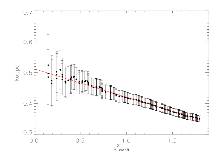
Figure 1: Extrapolation of the parameter $\kappa$ from a series of fittings with different $\tilde{q}^{2}_{\rm cutoff}$ using the power-law model with lattices: $V=16\times 16\times 32\times 80$, $\beta=1.9$.

Since the power-law behavior of $Z(\tilde{q}^{2})$ is expected to be valid only at small momenta, a cutoff $\tilde{q}^{2}_{\rm cutoff}>0$ should be placed on the momentum modes that are measured to set up the appropriate fitting range. Ideally, if we have enough low-momentum data points, the result of the fitting should not depend on the artificial cutoff parameter $\tilde{q}^{2}_{\rm cutoff}>0$. But if there were not enough low-momentum data points, the final result will have some dependence on the cutoff parameter, which turns out to be case of our study. To solve this problem, we have tried two methods in the fitting. In the first method, a series of fittings are performed with variable cutoff parameter $q^{2}_{\rm cutoff}$. The value of $\kappa$ are obtained for each of these fitting ranges. The final value of $\kappa$ is determined as a extrapolation in the limit $\tilde{q}^{2}_{\rm cutoff}\rightarrow 0$. The results for the value of $\kappa$ are illustrated in Figure 1, 2 and 3 for each set of lattice samples. The horizontal axis in these figures are the momentum cutoff parameters $\tilde{q}^{2}_{\rm cutoff}$. The data points are the fitted value of $\kappa$ up to the corresponding cutoff value. The red curves are the linear extrapolations of various values of $\kappa$ obtained at different $\tilde{q}^{2}_{\rm cutoff}$ towards the limit $\tilde{q}^{2}_{\rm cutoff}\rightarrow 0$. The extrapolated values at $\tilde{q}^{2}_{\rm cutoff}\rightarrow 0$ are the final estimates for $\kappa$ using this fitting method.

In the first row of the Figure 4, the data points for the dressing function $Z(\tilde{q}^{2})$ are plotted together with the corresponding power-law behavior fits (the red curve) using the extrapolated values of $\kappa$. The final extrapolated results for $\kappa$ are also tabulated in the first three rows of Table 2 together with the corresponding $\chi^{2}/d.o.f.$. The values for the anisotropy parameter $\xi_{R}=xi_{0}$ are obtained using the second fitting method to be described below. The resulting $\kappa$ values at $\tilde{q}^{2}_{\rm cutoff}\rightarrow 0$ are consistent with a finite propagator at zero momentum, i.e. $\kappa\simeq 0.5$ although more definite conclusions will require more accurate simulation results. It is also noted that the $\kappa$ values obtained from lattices with similar physical sizes (i.e. L12B19 and L16B22) but different lattice spacing are consistent with each other within the errors, showing that the value of $\kappa$ is not sensitive to lattice spacing errors after tadpole improvement. The $\kappa$ value from the lattice with a larger physical size (i.e. L16B19) is slightly larger from the smaller lattice results by about one standard deviation.

In the fitting method described above, the value of $\kappa$ can be estimated quite accurately in the IR region. However, since there are not so many low-momentum data points, the value of the renormalized anisotropy $\xi_{R}$ can not be obtained accurately. In order to accommodate more data points at larger momenta into our fitting procedure, we also adopted a second fitting method. In this second fitting method, we express the dressing function as the power-law behavior times a polynomial in $\tilde{q}^{2}$ to a certain order:a

$$Z(\tilde{q}^{2})\propto(\tilde{q}^{2})^{2\kappa}(1+a_{1}\tilde{q}^{2}+a_{2}\tilde{q}^{4}+\ldots)$$ (18)

Using this method, the gluon dressing functions for the three set of lattices are fitted again. The three plots in the second row of Fig. 4 illustrate the situation of this fitting. The results of this fitting procedure are listed in row 4, 5 and 6 of Table 2. The value of $\kappa$ obtained with this method is also consistent with a finite propagator at zero momentum, but with a larger compared with the results from the previous method. However, this method yields more robust values for the anisotropy $\xi_{R}$. Thus as a final step, we fix the $\xi_{R}$ values obtained from this second method and perform the fit of $\kappa$ using the first method. These results of $\kappa$ are listed in the first three rows of Table 2.

III.2 Fitting Propagator with Other Models

There are other ways of parameterizing the dressing function $Z(\tilde{q}^{2})$ cut_pole :

$$Z_{\rm cut}(\tilde{q}^{2})\propto(\frac{\tilde{q}^{2}}{\tilde{q}^{2}+\Lambda^{2}})^{2\kappa}$$ (19a)

$$Z_{\rm pole}(\tilde{q}^{2})\propto\frac{(\tilde{q}^{2})^{2\kappa}}{(\tilde{q}^{2})^{2\kappa}+(\Lambda^{2})^{2\kappa}}$$ (19b)

In these parameterizations, another parameter $\Lambda$ is introduced. Obviously, in the small $\tilde{q}^{2}$ region they agree with the previous models. Fitting to these two forms are also performed and the corresponding results are given in the last six rows of Table 2. The comparison of the fitted curve together with the data points are shown in the last two rows of Figure 4. The final results from these models are quite unstable for various lattices with large errors to the fitted parameters, both $\kappa$ and $\Lambda$. These results seem to be consistent with previous studies kappa595_1 ; kappa595_2 ; kappa595_3 . However, since the fitted parameters have large errors and the values are not quite consistent on various lattices, no definite conclusions should be made from this fitting method.

IV Conclusions

In this paper, the gluon propagator in Landau gauge are investigated using anisotropic lattices in the IR region. Improved lattice gauge actions are utilized which reduces the lattice artifacts substantially. We also used lattices with one of the spatial direction is twice as long as the other two spatial directions. The largest spatial size we used in this study is about $11$fm, allowing us to have more low-momentum modes into the infra-red region.

The momentum space gluon propagator measured in our lattice simulations are fitted using various models. The exponent $\kappa$, which characterize the power-law behavior of the gluon dressing function in the IR region, is found to be consistent with $0.5$. This implies that the gluon propagator may have a finite value at zero momentum, in agreement with the result using other non-lattice methods. This work also confirms that IR region gluon propagator can be well investigated by adopting improved gauge action and lattices with large volume and coarse anisotropic spacing.

Table 1: Lattice parameters.

Lattice	Beta	Physical size	Configurations
$16\times 16\times 32\times 80$	1.9	$5.65\times 5.65\times 11.30\times 5.65fm^{4}$	200
$16\times 16\times 32\times 80$	2.2	$4.47\times 4.47\times 8.95\times 4.47fm^{4}$	207
$12\times 12\times 24\times 60$	1.9	$4.24\times 4.24\times 8.48\times 4.24fm^{4}$	207

Table 2: Results for the gluon dressing function $Z(\tilde{q}^{2})$ from various fitting models.

Fit Patten	Parameters	$\xi_{R}/\xi_{0}$	$\kappa$	$\Lambda$	$\chi^{2}/d.o.f.$
Power-law	L16B19	fixed at $0.6135$	$0.5124\pm 0.0044$		$0.2054$
Power-law	L12B19	fixed at $0.6541$	$0.4976\pm 0.0097$		$0.2320$
Power-law	L16B22	fixed at $0.6667$	$0.4917\pm 0.0129$		$0.2473$
Power-law	L16B19	$0.6135\pm 0.0316$	$0.5117\pm 0.0305$		$0.0725$
Power-law	L12B19	$0.6541\pm 0.0261$	$0.4736\pm 0.0292$		$0.0834$
Power-law	L16B22	$0.6667\pm 0.0240$	$0.4461\pm 0.0258$		$0.0644$
$Z_{cut}$	L16B19	$0.5832\pm 0.0362$	$0.6745\pm 0.0808$	$0.5493\pm 0.1294$	$0.0782$
$Z_{cut}$	L12B19	$0.6379\pm 0.0306$	$1.0846\pm 0.3258$	$0.2127\pm 0.0868$	$0.1471$
$Z_{cut}$	L16B22	$0.6564\pm 0.0299$	$1.0808\pm 0.3261$	$0.1164\pm 0.0475$	$0.1278$
$Z_{pole}$	L16B19	$0.5874\pm 0.0354$	$0.6128\pm 0.0372$	$0.6913\pm 0.0743$	$0.0736$
$Z_{pole}$	L12B19	$0.6428\pm 0.0293$	$0.7630\pm 0.0639$	$0.4999\pm 0.0335$	$0.1234$
$Z_{pole}$	L16B22	$0.6583\pm 0.0286$	$0.7612\pm 0.0634$	$0.2763\pm 0.0182$	$0.1020$

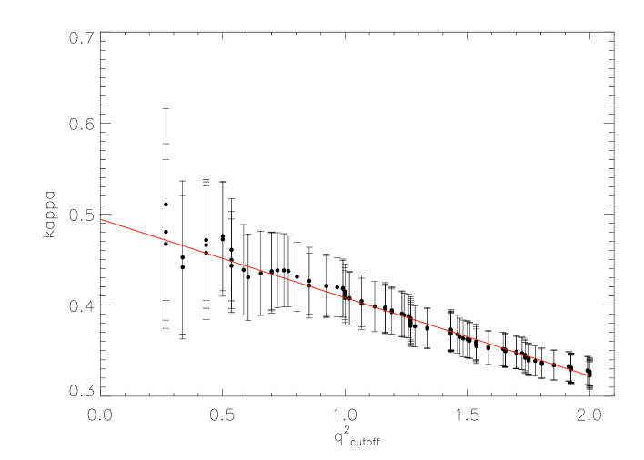
Figure 2: Extrapolation of the parameter $\kappa$ from a series of fittings with different $\tilde{q}^{2}_{\rm cutoff}$ using the power-law model with lattices: $V=12\times 12\times 24\times 60$, $\beta=1.9$.

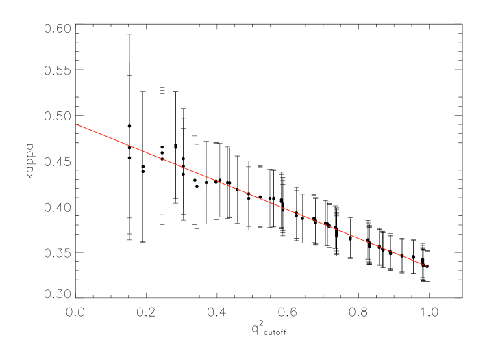
Figure 3: Extrapolation of the parameter $\kappa$ from a series of fittings with different $\tilde{q}^{2}_{\rm cutoff}$ using the power-law model with lattices: $V=16\times 16\times 32\times 80$, $\beta=2.2$.

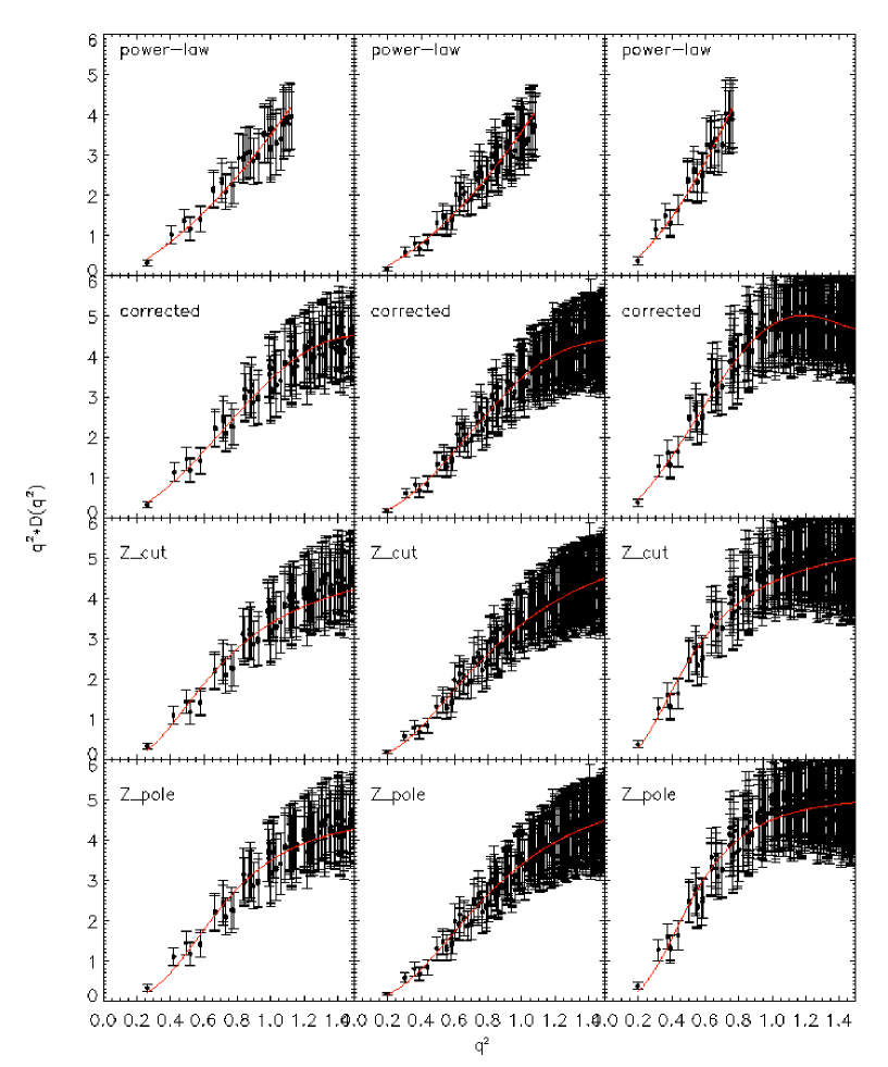
Figure 4: Fitting the gluon dressing function to various models.(with Eq. 17, Eq. 18, Eq. 19a and Eq. 19b respectively)

References

- (1) L. von Smekal, R. Alkofer and A. Hauck, Phys. Rev. Lett. 79 (1997) 3591 C3594, [hep-ph/9705242]; Ann. Phys. 267 (1998) 1, [hep-ph/9707327].
- (2) J. M. Pawlowski, D. F. Litim, S. Nedelko and L. von Smekal, Phys. Rev. Lett. 93 (2004) 152002, [hep-th/0312324].
- (3) D. Zwanziger, Phys. Rev. D65 (2002) 094039, [hep-th/0109224].
- (4) J. E. Mandula, M. Ogilvie, Phys. Lett. B185 (1987) 274.
- (5) J. E. Mandula, Phys. Rept. 315 (1999) 273 [hep-lat/9907020].
- (6) A. Cucchieri, T. Mendes, A. Taurines,Phys. Rev. D67 (2003) 091502 [heplat/0302022].
- (7) J. C. R. Bloch, A. Cucchieri, K. Langfeld, T. Mendes, Nucl. Phys. B687 (2004) 76 [hep-lat/0312036].
- (8) S. Furui, H. Nakajima, Phys. Rev. D69 (2004) 074505 [hep-lat/0305010].
- (9) A. Sternbeck, E.-M. Ilgenfritz, M. Muller-Preussker, A. Schiller, Phys. Rev. D72 (2005) 014507 [hep-lat/0506007].
- (10) D. B. Leinweber, J. I. Skullerud, A. G. Williams, C. Parrinello, Phys. Rev. D60 (1999) 094507; Erratum, Phys. Rev. D61 (2000) 079901 [hep-lat/9811027].
- (11) F. D. R. Bonnet, P. O. Bowman, D. B. Leinweber, A. G. Williams, J. M. Zanotti, Phys. Rev. D64 (2001) 034501 [hep-lat/0101013].
- (12) Christian S. Fischer [arXiv:0709.3205v1]
- (13) J.P. Ma, Mod.Phys.Lett. A15 (2000) 229-244 [hep-lat/9903009 v1]
- (14) A. Sternbeck et., PoS(LAT2006)076 [hep-lat/0610053 v1]
- (15) G.P. Lepage , P.B. Mackenzie, Phys. Rev. D 48, 2250 (1993).
- (16) K. Symanzik, Nucl. Phys. B 226, 187 (1983) ibid. pp. 205ff.
- (17) P. Weisz, Nucl. Phys. B 212, 1 (1983); P. Weisz , R. Wohlert, Nucl. Phys. B 236, 397 (1984); Erratum Cibid. B 247, 544 (1984).
- (18) M. Lücher and P. Weisz, Commun. Math. Phys. 97, 59 (1985).
- (19) Wei Liu , et., Mod.Phys.Lett. A21 (2006) 2313-2322 [hep-lat/0603015 v1]
- (20) Ying Chen, Bing He, He Lin, Ji-Min Wu, Mod.Phys.Lett. A15 (2000) 2245-2256 [arXiv:hep-lat/0008001v1]
- (21) O. Oliveira and P. J. Silva [hep-lat/0609036 v1]
- (22) Andre Sternbeck [hep-lat/0609016 v1]
- (23) Frédéric D.R. Bonnet, Patrick O. Bowman et., Phys.Rev. D64 (2001) 034501 [hep-lat/0101013 v2]
- (24) P. J. Silva. and O. Oliveira [hep-lat/0609069 v2]
- (25) D.B. Leinweber, J-I. Skullerud, A.G.Williams , C. Parrinello, Phys. Rev. D 58, 031501 (1998); ibid. D 60, 094507 (1999); Erratum Cibid. D 61, 079901 (2000).
- (26) R. Alkofer, W. Detmold, C. S. Fischer, P. Maris, Phys. Rev. D70 (2004) 014014 [hep-ph/0309077].
- (27) L. von Smekal, R. Alkofer and A. Hauck, Phys. Rev. Lett. 79 (1997) 3591.
- (28) D. Zwanziger, Phys. Rev. D 65 (2002) 094039; Phys. Rev. D 69, 016002 (2004).
- (29) Ch. Lerche and L. von Smekal, Phys. Rev. D 65 (2002) 125006.
- (30) J. M. Pawlowski, D. F. Litim, S. Nedelko and L. von Smekal, Phys. Rev. Lett. 93 (2004) 152002; AIP Conf. Proc. 756 (2005) 278.