Behavior of tachyon in string cosmology based on gauged WZW model

$\rm{Sunggeun\,\,Lee}^{{\dagger}}$  and $\rm{Soonkeon\,\,Nam}^{\P}$

†Center for Quantum Spacetime, Sogang University, Seoul 121-742, Korea
¶Department of Physics and Research Institute for Basic Sciences, Kyung Hee University, Seoul 130-701, Korea

Abstract

We investigate a string theoretic cosmological model in the context of the gauged Wess-Zumino-Witten model. Our model is based on a product of non-compact coset space and a spectator flat space; $[SL(2,R)/U(1)]_{k}\times{\bf R}^{2}$. We extend the formerly studied semiclassical consideration with infinite Kac-Moody level $k$ to a finite one. In this case, the tachyon field appears in the effective action, and we solve the Einstein equation to determine the behavior of tachyon as a function of time. We find that tachyon field dominates over dilaton field in early times. In particular, we consider the energy conditions of the matter fields consisting of the dilaton and the tachyon which affect the initial singularity. We find that not only the strong energy but also the null energy condition is violated.

1 Introduction

As a strong candidate for a theory of quantum gravity, string theory should explain our universe near the big bang, and should resolve the initial singularity of the standard cosmology [1]. Although a lot of effort has been made to get reasonable answers, there are still more questions than answers. One of the challenges of string cosmology [2, 3, 4] is that, in general, string theory is quite useful for static problems but for time dependent cases it becomes much harder. For instance, string theory is quite useful for resolutions of orbifold [5, 6] or conifold singularities [7], or for explaining black hole entropy for extremal black holes [8], but it has not been as successful in explaining black hole singularity itself or time dependent cosmological models [9, 10].

Nevertheless, the cosmological model in string theory can be studied in various ways. One of them is to solve the Einstein equation from the low energy effective action which comes from the vanishing beta function for conformal invariance of two dimensional string worldsheet action. Another one, which is more stringy, is to study Wess-Zumino-Witten (WZW) action [12, 13] on a coset manifold which is a gauged version of WZW model[14, 15]. In the approach using the effective string action, it is hard to see all the stringy effects. It does not capture $\alpha^{\prime}$ corrections to all orders. In fact, solving the Einstein equations with all higher $\alpha^{\prime}$ corrections is very hard except in theories with enough SUSY to cancel the higher derivative terms (when the non-renormalization theorem kicks in). On the other hand, the method based on the gauged WZW model captures physics to all orders of $\alpha^{\prime}$ naturally.

One exact model for strings on a curved spacetime was a model by Witten which is a gauged WZW model on $SL(2,R)/U(1)$ coset manifold [16]. The target space of this background is a two dimensional black hole. This model was further studied by Dijkgraaf, Verlinde, and Verlinde [20] for the case of finite $k$. Moreover, it can be extended to higher dimensions [17]. Utilizing this solution, a four dimensional string theoretic cosmological model was also studied by taking products of two cosets $[SL(2,R)/U(1)]_{k_{1}}\times[SU(2)/U(1)]_{k_{2}}$ [18]. A very interesting cosmological model based on gauged WZW model was introduced by Kounnas and Lüst [19] who studied $[SL(2,R)/U(1)]_{k}\times{\bf R}^{2}$, and by taking the level $k$ negative. In this model, the singularity is absent, because it is hidden behind the horizon.

As mentioned above, the advantage of studying the WZW model is that it provides an exact solution to all orders in $\alpha^{\prime}$. This model has a correction through the Kac-Moody level $k$ by $1/k$. Considering the leading order term in $1/k$ expansion is equivalent to considering the problem in semiclassical limit. With the stringy background obtained from the gauged WZW model in leading order $1/k$, Kounnas and Lüst studied the effect of the dilaton field using the effective action. This means that, while the usual string effective action should be checked to all higher orders in $\alpha^{\prime}$ for requiring exact CFT (vanishing beta function), the WZW action is correct for all $\alpha^{\prime}$, the only correction is in terms of level $k$.

In this paper we extend the work of Kounnas and Lüst to all orders in $1/k$. We find the cosmological metric for finite $k$ by taking $k$ negative of the metric in Refs. [20, 21]. The gauged WZW model provides an exact stringy background, and we will study the effects of fields in the background. We include extra two dimension as was done in Ref. [19] to study as a four dimensional cosmology. After setting up the model, we solve the cosmological model in the four dimensional effective action including the tachyon as well as the dilaton. Especially, the time dependence of the tachyon is considered.

The rest of the paper is organized as follows: In section II we review the model by Kounnas and Lüst which is the case of semiclassical consideration. In section III we discuss the case of finite $k$, and also consider the effect of tachyon in the background. We study various energy conditions applied to the matter fields (dilaton and tachyon) in this case. In section IV we conclude with discussions.

2 Kounnas and Lüst model: $k\to\infty$ case

In this section, we briefly review the work of Kounnas and Lüst[19]. They considered a gauged WZW model based on the coset $[SL(2,R)/U(1)]_{k}\times{\bf R}^{2}$. The gauged WZW model on the coset $G/H$ is basically described by the following action [14, 15]:

$$S = {k\over{4\pi}}\int d^{2}z(g^{-1}\partial gg^{-1}\bar{\partial}g)-{k\over{12\pi}}\int_{B}tr(g^{-1}dg\wedge g^{-1}dg\wedge g^{-1}dg)$$ (1)

$$+ {k\over{2\pi}}\int d^{2}ztr(A\bar{\partial}gg^{-1}-\bar{A}g^{-1}\partial g-g^{-1}Ag\bar{A}^{-1}).$$

Here, the boundary of $B$ is the 2 dimensional worldsheet, $g$ is a group element of the group $G$, and $A$ is the gauge field of $H$, which is a subgroup of $G$. The level of the Kac-Moody algebra for the group of $G$ is $k$. Here $\partial$ and $\bar{\partial}$ denote partial integration with respect to the complex world sheet coordinates $z$ and $\bar{z}$, respectively.

The central charge of the WZW model on the compact $SU(2)/U(1)$ coset is $c=3k/(k+2)-1$, while for noncompact coset $SL(2,R)/U(1)$ it is $c=3k/(k-2)-1$. For the WZW model on the coset $[SL(2,R)/U(1)]\times{\bf R}^{2}$, we get central charge $c=3k/(k-2)-1+2=4+6/(k-2)$.

We can parametrize $G=SL(2,R)$ as

$$g=\left(\begin{array}[]{cc}u&a\\ -b&v\\ \end{array}\right)$$ (2)

Choosing a gauge with $a=\pm b$, the action can be written as a sigma model action of the form

$$S=\int d^{2}zg_{\mu\nu}(X)\partial X^{\mu}\bar{\partial}X^{\nu}.$$ (3)

That is, the gauged WZW model describes strings moving on some coset manifold with the target space described by coordinate $X^{\mu}$ with spacetime metric $g_{\mu\nu}(X)$. After fixing the gauge, we see that the WZW model is reduced to a non-linear sigma model. For example, for the coset $SL(2,R)/U(1)$, the target space is a black hole described by a metric [16]

$$ds^{2}=-k{dudv\over{1-uv}}.$$ (4)

If we are interested in four dimensional target spacetime, the simplest case is when we include two extra flat dimensions ${\bf R}^{2}$. The coset is now $[SL(2,R)/U(1)]\times{\bf R}^{2}$ and for the semiclassical limit $k\to\infty$, the four dimensional sigma model metric is

$$ds_{\sigma}^{2}=-k{dudv\over{1-uv}}+dx_{2}^{2}+dx_{3}^{2},$$ (5)

where $x_{2}$ and $x_{3}$ are the coordinates of ${\bf R}^{2}$. So the metric describes a two dimensional black hole background with two spectator dimensions. If we introduce coordinates $x_{0}$ and $x_{1}$ such that

$$u=e^{x_{1}}\sinh x_{0},~{}~{}~{}{\rm and}~{}~{}~{}v=-e^{-x_{1}}\sinh x_{0},$$ (6)

we get another form of the metric:

$$ds^{2}=-k(-dx_{0}^{2}+\tanh^{2}x_{0}dx_{1}^{2})+dx_{2}^{2}+dx_{3}^{2}.$$ (7)

Near $x_{0}\to 0$, the dilaton vanishes and the metric becomes completely smooth, being flat, when $x_{0}$ is non-compact. The spacetime is a product of two dimensional Milne universe times ${\bf R}^{2}$ [23]. Although $t=0$ is non-singular, this is as close as we can get to the big bang singularity in this model. In order to have a time dependent cosmological background, we need to make $x_{0}$ coordinate timelike. So we will denote $x_{0}$ as $t$. This is achieved by making the level $k$ negative. As we can see from the scale factor, $\tanh^{2}t$, this cosmological metric is not good for realistic cosmology such as for inflationary. The scale factor saturates at late times. However, the metric could describe the spacetime near the big bang. Since our starting point is a gauged WZW model which has stringy nature in itself, we might expect to have a resolution of the singularity. Indeed, in the model of Kounnas and Lüst, by taking negative $k$, they could obtain singularity free spacetime background. Choosing negative $k$ has an effect of rotating the Penrose diagram of the black hole. As a result, the big bang singularity is hidden behind what used to be the black hole horizon. Hence, from now on, we take $k$ as negative and rename $-k$ as $k$. Taking negative Kac-Moody level may give rise to non-unitarity but it is not solved completely [30, 31]. We ignored this issue in the present work.

By requiring conformal invariance of the non-linear sigma model, i.e., vanishing of the beta function, we get the four dimensional effective action for the graviton $g_{\mu\nu}$ and the dilaton $\phi$ background. In string frame it is given by the following action [22]:

$$S=\int d^{4}x\sqrt{-det(g_{\mu\nu})}e^{-\phi}\left(R+(\nabla\phi)^{2}+\Lambda\right),~{}~{}~{}~{}~{}\Lambda=-4/(k+2),$$ (8)

Here, $\Lambda$ which plays the role of cosmological constant, and we have put $8\pi G=1$, where $G$ is the Newton’s constant. The dilaton is given by

$$\phi=-\log(1-uv)=-\log(1+\sinh^{2}t)=-\log(\cosh^{2}t),$$ (9)

such that $e^{\phi}=1/\cosh^{2}t$.

The Einstein equations which follow from the action are:

$$R_{\mu\nu}+\nabla_{\mu}\nabla_{\nu}\phi=0,$$

$$R-(\nabla_{\mu}\phi)^{2}+2\nabla_{\mu}\nabla^{\mu}\phi+\Lambda=0.$$ (10)

Now let us consider the equation in the Einstein frame. We can get the Einstein frame action by conformal transformation $g_{E,\mu\nu}=e^{-\phi}g_{Str,\mu\nu}$. As a result we get the Einstein frame action

$$S=\int d^{4}x\sqrt{-det(g_{\mu\nu})}\left(R-{1\over 2}(\nabla\phi)^{2}-e^{\phi}{4\over{k+2}}\right).$$ (11)

The Einstein equation is

$$R_{\mu\nu}-{1\over 2}g_{\mu\nu}R=T^{\phi}_{\mu\nu},$$ (12)

where

$$T^{\phi}_{\mu\nu}={1\over 2}\nabla_{\mu}\phi\nabla_{\nu}\phi-{1\over 4}g_{\mu\nu}(\nabla\phi)^{2}-{2\over{k+2}}e^{\phi}g_{\mu\nu}.$$ (13)

In the Einstein frame, the metric is now given by

$$ds^{2}=\cosh^{2}t\left[(k+2)(-dt^{2}+\tanh^{2}tdx_{1}^{2})+dx_{2}^{2}+dx_{3}^{2}\right].$$ (14)

We find that this metric is non-singular. In order to check this, we calculate the scalar curvature which is given as follows:

$$R=-{{(\sinh^{2}t+2)}\over{2(\sinh^{2}t+1)}}.$$ (15)

This metric is obviously nonsingular as $t\to 0$. As we expected, string theory prevents initial big bang singularity in this model.

Now let us see the behavior of the dilaton field. It is quite illuminating to check the energy conditions. There is a theorem by Hawking and Penrose [1] which states that there must be a singularity when the strong energy condition, $\rho+3p\geq 0$ is satisfied. Here, we expect to find the violation of this energy condition. Now, let us calculate the components of the stress energy tensor $T_{00}$ and $T_{ii}$ to check energy conditions.

$$T^{\phi}_{00}={1\over 2}\nabla_{0}\phi\nabla_{0}\phi-{1\over 4}g_{00}\nabla_{0}\phi\nabla_{0}\phi g^{00}-{2\over{k+2}}g_{00}e^{\phi}={{3\tanh^{2}t+2}\over{(1+\tanh^{2}t)^{2}}}=\rho,$$ (16)

and

$$T^{\phi}_{ii}={1\over 2}\nabla_{i}\phi\nabla_{i}\phi-{1\over 4}g_{ii}(\nabla\phi)^{2}-{2\over{k+2}}e^{\phi}g_{ii}=g_{ii}\left(-{1\over 4}g^{00}\dot{\phi}^{2}-{2\over{k+2}}e^{\phi}\right)$$

$$~{}~{}~{}=g_{ii}{1\over{k+2}}{{-\tanh^{2}t-2}\over{(1+\tanh^{2}t)^{2}}}=pg_{ii}.$$ (17)

We can absorb the $1/(k+2)$ into the metric such that $T^{\phi}_{ii}=g_{ii}(-\tanh^{2}t-2)/(1+\tanh^{2}t)^{2}$.

For our further consideration of energy conditions we summarize the four energy conditions, null (NEC), weak (WEC), strong (SEC), and dominant (DEC) energy conditions:

$${\rm NEC}:~{}\rho+p\geq 0,$$

$${\rm WEC}:~{}\rho\geq 0~{}~{}{\rm and}~{}~{}\rho+p\geq 0,$$

$${\rm SEC}:~{}\rho+3p\geq 0~{}~{}{\rm and}~{}~{}\rho+p\geq 0,$$

$${\rm DEC}:~{}\rho\geq 0~{}~{}{\rm and}~{}~{}\rho\pm p\geq 0.$$ (18)

If we check the weak energy condition and strong energy condition for Kounnas and Lüst model, we have the following:

$${\rm WEC}:~{}\rho+p={2\tanh^{2}t\over{(1+\tanh^{2}t)^{2}}}>0,$$

$${\rm SEC}:~{}\rho+3p=-{4\over{(1+\tanh^{2}t)^{2}}}<0.$$ (19)

We see that only the strong energy condition is violated. Below we draw a picture for both energy conditions.

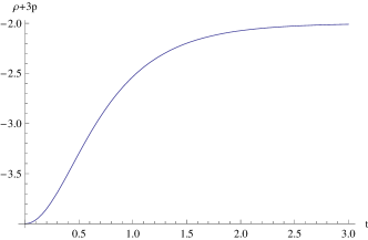
Figure 1: The behavior of $\rho+p$ and $\rho+3p$. We see that $\rho+3p$ is definitely negative and violates weak energy condition.

The violation of the strong energy condition is consistent with the absence of the big bang singularity of the background geometry.

3 The behavior of tachyon field: finite level $k$

We now consider the same coset model considered by Kounnas and Lüst, but with the metric corrected by finite value of $k$. The metric for the $[SL(2,R)/U(1)]_{k}$ WZW model with finite $k$ was studied in Refs. [20, 21]. Again we include extra two directions $x_{2}$ and $x_{3}$ such that we have $[SL(2,R)/U(1)]\times{\bf R}^{2}$ coset space to study four dimensional spacetime but they do not play much role. To get a cosmological metric we take $k$ negative. As a result we get the the metric in Einstein frame which is given by the following:

$$ds^{2}=\left(\cosh^{2}t\sqrt{1+{2\over k}\tanh^{2}t}\right)\left[{{k+2}\over 2}\left(-dt^{2}+{1\over{\coth^{2}t+{2\over k}}}dx_{1}^{2}\right)+dx_{2}^{2}+dx_{3}^{2}\right].$$ (20)

The dilaton $\phi$ is given by

$$e^{-\phi}=\cosh^{2}t\sqrt{1+{2\over k}\tanh^{2}t}.$$ (21)

As $k\to\infty$, $e^{\phi}$ reduces to Eq.(9). As in the case of semiclassical approach $k\to\infty$, the metric is obviously singularity free. In fact, we have checked that the metric has no singularity, with the help of ${\rm Mathematica}^{\rm TM}$. The expression is to complicated and we will not write it down here. The string coupling constant, $g_{s}\sim e^{\phi}$, becomes weak as time flows to future with initially finite value.

Now that the spacetime action contains the tachyon ${\cal T}$ we would like to see the time dependent behavior of tachyon field. The action in Einstein frame with the tachyon is given by [24, 25]

$$S=\int d^{4}x\sqrt{-det(g_{\mu\nu})}\left(R-{1\over 2}(\nabla\phi)^{2}+\lambda e^{\phi}+(\nabla{\cal T})^{2}-V({\cal T})e^{\phi}\right),~{}~{}~{}\lambda=-{4\over{k+2}}.$$ (22)

Here $V({\cal T})$ is a tachyon potential whose exact form is not necessary. It is hard to solve the Einstein equations of motion from this action. However, since the metric was already determined by fixing the coset manifold, we just need to find the tachyon field as a function of time by solving the Einstein equations of motion of this action. For this we will assume that all the fields including the tachyon field ${\cal T}$ depends only on the time $t$.

By varying the above action, we get field equations including the Einstein equations, which are given by

$$R_{\mu\nu}-{1\over 2}g_{\mu\nu}R$$

$$~{}~{}~{}~{}~{}={1\over 2}\nabla_{\mu}\phi\nabla_{\nu}\phi-{1\over 4}g_{\mu\nu}(\nabla\phi)^{2}+{\lambda\over 2}g_{\mu\nu}e^{\phi}-{1\over 2}g_{\mu\nu}e^{\phi}V({\cal T})-\nabla_{\mu}{\cal T}\nabla_{\nu}{\cal T}+{1\over 2}g_{\mu\nu}(\nabla{\cal T})^{2}$$

$$\ \ \ \ \ \ =T^{\phi}_{\mu\nu}+T^{\cal T}_{\mu\nu}=T_{\mu\nu},$$

$$\nabla^{2}\phi+\left(\lambda-V({\cal T})\right)e^{\phi}=0,$$

$$-2\nabla^{2}{\cal T}-{d\over{d{\cal T}}}V({\cal T})e^{\phi}=0.$$ (23)

To find the time dependent behavior of the tachyon ${\cal T}$, we put the solutions for metric and the dilaton into the above equations. However, it is still quite hard to solve them analytically. So, we take approximations and see the asymptotic behavior of the tachyon field. Another thing to check is that since the metric has no singularity, we have to check to see whether the weak- and strong-energy conditions violate or not.

The energy momentum tensor can be read from above after some calculation. With the help of the equations of motions (23), $T_{00}$ and $T_{ii}$ can be reduced to the following:

$$T_{00}={1\over 4}{\dot{\phi}}^{2}-{1\over 2}g_{00}\nabla^{2}\phi-{1\over 2}{\dot{\cal T}}^{2},$$

$$T_{ii}=-{1\over 4}g_{ii}g^{00}{\dot{\phi}}^{2}-{1\over 2}g_{ii}\nabla^{2}\phi+{1\over 2}g_{ii}g^{00}{\dot{\cal T}}^{2},$$ (24)

where we have denoted the time derivative $d\over dt$ by $\cdot$. Moreover, due to the explicit form of the dilaton $\phi$ in Eq.(21), we just need to know the $\dot{\cal T}$ in order to determine $T_{00}$ and $T_{ii}$.

Since we can put

$${d\over{d{\cal T}}}V=\dot{V}/\dot{\cal T},~{}~{}~{}{\rm and}~{}~{}~{}\dot{V}={d\over{dt}}(e^{-\phi}\nabla^{2}\phi)=-\dot{\phi}e^{-\phi}\nabla^{2}\phi+e^{-\phi}{d\over{dt}}(\nabla^{2}\phi),$$ (25)

we need to solve the following equation to get the equation for $\dot{\cal T}$:

$$-2\dot{\cal T}={\dot{V}e^{\phi}\over\nabla^{2}{\cal T}}\ \ \ \ \ \ \leftrightarrow\ \ \ \ \ \ \dot{\cal T}e^{-\phi}\nabla^{2}{\cal T}=-{1\over 2}\dot{V}=-{1\over 2}{d\over{dt}}(e^{-\phi}\nabla^{2}\phi).$$ (26)

In other words, the tachyon ${\cal T}$ satisfies the following equation:

$$\dot{\cal T}e^{-\phi}\nabla^{2}{\cal T}=-{1\over 2}{d\over{dt}}(e^{-\phi}\nabla^{2}\phi),$$ (27)

which reads

$$\ddot{\cal T}+{\dot{f}\over f}\dot{\cal T}=-{1\over 2}{1\over{\dot{\cal T}}}{d\over{dt}}\left(\ddot{\phi}+{\dot{f}\over f}\dot{\phi}\right).$$ (28)

In the above we have introduced

$$f(t)=g^{00}\sqrt{-\det(g)}=-\sinh t\cosh t.$$ (29)

The time dependence of the tachyon potential, $V(t)$, satisfies the following differential equation:

$$\dot{V}={d\over{dt}}\left[-{2\over{k+2}}{1\over{fg}}g\left(\dot{f}\dot{\phi}+f\ddot{\phi}\right)\right]=-{2\over{k+2}}{d\over{dt}}\left(\ddot{\phi}+{\dot{f}\over f}\dot{\phi}\right).$$ (30)

In terms of known functions $f(t)$ and $\phi(t)$ in Eqs.(9) and (23), we can rewrite the $T_{00}$ and $T_{ii}$ as

$$T_{00} = {1\over 4}{\dot{\phi}}^{2}-{1\over 2}(\ddot{\phi}+{\dot{f}\over f}\dot{\phi})-{1\over 2}{\dot{\cal T}}^{2},$$

$$T_{ii} = -{1\over 4}g_{ii}g^{00}{\dot{\phi}}^{2}+{1\over 2}g_{ii}(-\nabla^{2}\phi)+{1\over 2}g_{ii}g^{00}{\dot{\cal T}}^{2}$$ (31)

$$= g_{ii}\left(-{1\over 4}g^{00}{\dot{\phi}}^{2}-{1\over 2}\nabla^{2}\phi+{1\over 2}g^{00}{\dot{\cal T}}^{2}\right)$$

$$= g_{ii}e^{\phi}\left({1\over 4}{\dot{\phi}}^{2}+{1\over 2}(\ddot{\phi}+{\dot{f}\over f}\phi)\right)-g_{ii}e^{\phi}{1\over 2}{\dot{\cal T}}^{2},$$

where we absorbed ${2\over{k+2}}$ into the metric, and used the following relation:

$$g_{00}\nabla^{2}\phi=\ddot{\phi}+{\dot{f}\over f}\dot{\phi}.$$ (32)

For later convenience, we calculate the following expressions:

$$(\dot{\phi})^{2}={{4\tanh^{2}t(2+k-\cosh^{-2}t)^{2}}\over{(k+2\tanh^{2}t)^{2}}},$$

$${\dot{f}\over f}=\coth t+\tanh t,$$

$${d\over{dt}}\left(\ddot{\phi}+{\dot{f}\over f}\dot{\phi}\right)=F(t),$$ (33)

where

$$F(t)\equiv-{{(12+4k+3k^{2}+4(k^{2}-4)\cosh 2t+(2+k)^{2}\cosh 4t)\cosh^{-4}t}\over{2(k+2\tanh^{2}t)^{2}}}.$$ (34)

Now, $T_{00}$ and $T_{ii}$ can be expressed as follows:

$$T_{00}=\rho=\rho^{-}-{1\over 2}{\dot{\cal T}}^{2},$$

$$T_{ii}=g_{ii}p=g_{ii}p^{-}-g_{ii}e^{\phi}{1\over 2}{\dot{\cal T}}^{2}.$$ (35)

where

$$\rho^{-}\equiv{{3(2+k)^{2}-(2+k)(12+k)\cosh^{-2}t+(13+4k)\cosh^{-4}t-\cosh^{-6}t}\over{(k+2\tanh^{2}t)^{2}}},$$

$$p^{-}\equiv{-{\cosh^{-2}t((2+k)^{2}+(k-4)(2+k)\cosh^{-2}t+3\cosh^{-4}t+\cosh^{-6}t)}\over{(k+2\tanh^{2}t)^{2}(1+{2\over k}\tanh^{2}t)^{1\over 2}}}.$$ (36)

Now let us consider solving the differential equations for tachyon and obtain the behavior of the tachyon field. We have to solve the following equation:

$$\ddot{\cal T}+{\dot{f}\over f}\dot{\cal T}=-{1\over{\dot{\cal T}}}{d\over{dt}}\left(\ddot{\phi}+{\dot{f}\over f}\dot{\phi}\right),$$ (37)

which can also be rewritten as

$$\ddot{\cal T}+(\coth t+\tanh t)\dot{\cal T}=-{1\over 2}{1\over{\dot{\cal T}}}F(t).$$ (38)

This differential equation is the Bernoulli differential equation:

$$\dot{\cal G}-P(t){\cal G}=Q(t){\cal G}^{n}$$ (39)

where for ${\cal G}={\dot{\cal T}}$ the solution is given by

$${\cal G}^{1-n}=ce^{F}+(1-n)e^{F}\int e^{-F}Q(t)dt,$$ (40)

where

$$F=(1-n)\int P(t)dt.$$ (41)

This equation is still hard to solve analytically in our case. Hence, we take two opposite limits to see the asymptotic behavior. In the limit, $t\to\infty$, and $t\to 0$, this equation simplifies a lot.

$$t\to\infty:~{}~{}\ddot{\cal T}+2\dot{\cal T}={2\over{\dot{\cal T}}},$$

$$t\to 0:~{}~{}\ddot{\cal T}+t^{-1}\dot{\cal T}={{2(1+k)}\over k}{1\over\dot{\cal T}}.$$ (42)

The first equation has a solution

$${\dot{\cal T}}^{2}=1+e^{-4(t-t_{0})},$$ (43)

and the solution for the second equation is

$${\dot{\cal T}}^{2}={c\over t^{2}}+{4\over 3}{{k+1}\over k}t,$$ (44)

where $t_{0}$ and $c$ are integration constants. When we assume the tachyon field is a real value then $c$ is a positive constant.

We note that the tachyons becomes negligible in later times. The important contribution of the tachyons are in the early time near big bang ($t\sim 0$). In fact, it dominates over other fields for the contributions to $\rho$ and $p$. Due to tachyons, both $\rho$ and $p$ become negative values. Hence, we see that even the null energy condition is violated.

With the given energy momentum tensor we see that the conditions are calculated as follows for both null $p+\rho$ and strong $3p+\rho$:

$${\rm NEC}:~{}\rho+p=\rho^{-}+p^{-}-{1\over 2}{\dot{\cal T}}^{2}\left(1+\cosh^{-2}t(1+{2\over k}\tanh^{2}t)^{-{1\over 2}}\right),$$

$${\rm SEC}:~{}\rho+3p=\rho^{-}+3p^{-}-{1\over 2}{\dot{\cal T}}^{2}\left(1+3\cosh^{-2}t(1+{2\over k}\tanh^{2}t)^{-{1\over 2}}\right).$$ (45)

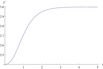
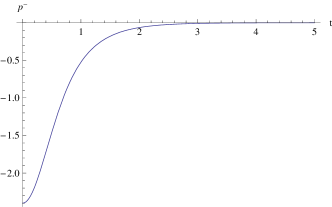
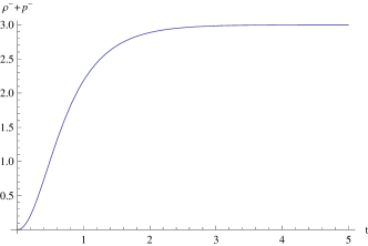
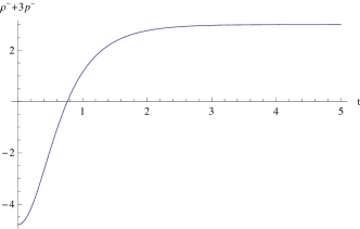
Figure 2: The behavior of $\rho^{-}$, $p^{-}$, $\rho^{-}+p^{-}$ and $\rho^{-}+3p^{-}$ as a function of time. In these diagrams the kinetic term of the tachyon is not involved but the contribution of the tachyon. The energy density is definitely negative.

In figure 2, we plot the $\rho$, $p$, $\rho+p$ and $\rho+3p$ below. The kinetic term of the tachyon, $\sim\dot{\cal T}^{2}$, is not involved temporarily. The only effect of tachyon comes from the potential. The tachyonic contribution is dominant near the big bang $t\sim 0$ and is negligible in later time. Here we have violation of the null energy condition as well as the violation of the strong energy condition. This is again consistent with the absence of the initial big bang singularity of the background geometry. In Ref.[26], the authors discussed that for the graceful exit the matter that violates the null energy condition is necessary. We would like to comment on the violation of the null energy condition. It seems that the violation of the null energy condition when the tachyon dominates does not seem to be problematic. Tachyon is just a signal of instability. We can interpret this tachyon as a supplementary matter for wormhole [27, 28, 29] which mediates the topology change near the big bang. It is believed that the wormhole ia a part of the space time foam bubbling near the big bang which quantum mechanical picture is quite necessary. So our model seems to provide useful ingredient for the early universe.

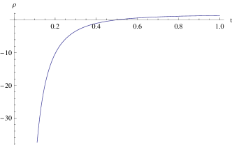
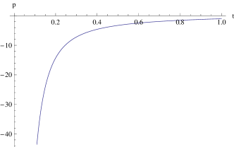
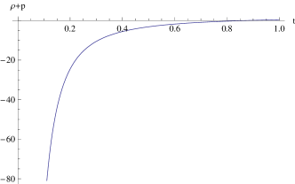
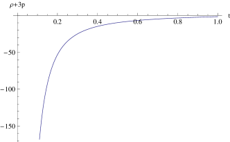
Figure 3: The behavior of $\rho$, $p$, $\rho+p$ and $\rho+3p$ at $t\sim 0$ with the inclusion of tachyon kinetic term. Note that the energy density itself is negative due to tachyon effect. In addition, both the strong and null energy condition are violated.

In figure 3, we plot the $\rho$, $p$, $\rho+p$ and $\rho+3p$ again including the tachyon kinetic contribution. Because of negligible tachyon effect in later time, we only focus on the times near big bang $t\sim 0$. Here we notice that in addition to the violation of the both strong and weak energy conditions, the energy density itself becomes negative near the big bang where the tachyon effect is formidably big.

4 Conclusion

In this paper, we studied the behavior of the tachyon in a cosmology based on the gauged WZW model. The cosmological metric is obtained by taking the negative sign of the Kac-Moody level $k$. We used the smooth, singularity free metric obtained in Refs.[17, 20, 21]. Next, we considered the behavior of tachyon field in the metric and the dilaton background by solving the equation of motion of the effective action. Although, the fully explicit solution could in principle be found by solving the Bernoulli differential equaion, we found on the initial ($t\to 0$) and asymptotic ($t\to\infty$) bahevior of the tachyon field. We find that tachyon field dominates in early tims. We could then calculate the components of the energy momentum tensor, $T_{00}$ and $T_{ii}$, and checked the energy conditions in connection to the singularity theorem. Contrary to the result of Kounnas and Lüst[19] where only the strong energy condition was violated, we have the strong as well as the null energy conditions violated near big bang ($t\sim 0$), where the tachyon dominates. It seems that the tachyon domination in the early universe might support understand the wormholes in the early universe, which is believed to be a space time foam.

Our consideration can be applied to other backgrounds such as Nappi-Witten model [18]. Moreover, we can consider other coset models or inclusion other fields such as antisymmetric tensor fields. It is also interesting to see the topology changing studied in Ref.[32]

5 Acknowledgements

This work was supported by the Science Research Center Program of the Korea Science and Engineering Foundation through the Center for Quantum Spacetime(CQUeST) of Sogang University with grant number R11 - 2005 - 021. It was also supported by the Korea Research Foundation Grant funded by the Korean Government(MOEHRD) (KRF-2007-314-C00056 ).

References

- [1] S. W. Hawking and G. F. R. Ellis, ”The large scale of space-time,” Cambridge Univ. Press, Cambridge, 1973.
- [2] M. Gasperini, “Elements of string cosmology,” Cambridge Univ. Press, Cambridge, 2007.
- [3] F. Quevedo, Class. Quant. Grav. 19 (2002) 5721.
- [4] G. Veneziano, hep-th/0002094 and references therein.
- [5] L. J. Dixon, J. A. Harvey, C. Vafa and E. Witten, Nucl. Phys. B 261 (1985) 678.
- [6] L. J. Dixon, J. A. Harvey, C. Vafa and E. Witten, Nucl. Phys. B 274 (1986) 285.
- [7] A. Strominger, Nucl. Phys. B 451 (1995) 96.
- [8] A. Strominger and C. Vafa, Phys. Lett. B 379 (1996) 99.
- [9] B. Craps, Class. Quant. Grav. 23 (2006) S849.
- [10] L. Cornalba and M. S. Costa, Fortsch. Phys. 52 (2004) 145 and references therein.
- [11] S. D. Mathur, Fortsch. Phys. 53 (2005) 793.
- [12] E. Witten, Commun. Math. Phys. 92 (1984) 455.
- [13] D. Gepner and E. Witten, Nucl. Phys. B 278, 493 (1986).
- [14] K. Bardacki, E. Rabinovici and B. Saering, Nucl. Phys. B 301 (1988) 151.
- [15] D. Karabali and H. J. Schnitzer, Nucl. Phys. B 329 (1990) 649.
- [16] E. Witten, Physi. Rev. D 44 (1991) 314.
- [17] K. Sfetsos, Phys. Rev. D 46 (1992) 4510.
- [18] C. R. Nappi and E. Witten, Phys. Lett. B 293 (1992) 309.
- [19] C. Kounnas and D. Lüst, Phys. Lett. B 289 (1992) 56.
- [20] R. Dijkgraaf, H. L. Verlinde and E. P. Verlinde, Nucl. Phys. B 371 (1992) 269.
- [21] K. Sfetsos, Nucl. Phys. B 389 (1993) 424.
- [22] C. G. Callan, E. J. Martinec, M. J. Perry and D. Friedan, Nucl. Phys. B 262 (1985) 593.
- [23] B. Craps, D. Kutasov and G. Rajesh, JHEP 0206 (2002) 053.
- [24] A. A. Tseytlin, Phys. Lett. B 264 (1991) 311.
- [25] K. Ghoroku, Phys. Lett. B 347 (1995) 21.
- [26] R. Brustein and R. Madden, Phys. Lett. B 410 (1997) 110.
- [27] M. S. Morris, K. S. Thorne and U. Yurtsever, Phys. Rev. Lett. 61 (1988) 1446.
- [28] C. W. Misner and J. A. Wheeler, Annals Phys. 2 (1957) 525.
- [29] J. A. Wheeler, Annals Phys. 2 (1957) 604.
- [30] L. J. Dixon, M. E. Peskin and J. D. Lykken, Nucl. Phys. B 325 (1989) 329.
- [31] S. Hwang, Nucl. Phys. B 354 (1991) 100.
- [32] E. Kiritsis and C. Kounnas, Phys. Lett. B 331 (1994) 51.