2D non-LTE radiative modelling of He I spectral lines formed in solar prominences

Abstract

Context. The diagnosis of new high-resolution spectropolarimetric observations of solar prominences made in the visible and near-infrared mainly, requires a radiative modelling taking into account for both multi-dimensional geometry and complex atomic models.

Aims. Hereafter we contribute to the improvement of the diagnosis based on the observation of He i multiplets, by considering 2D non-LTE unpolarized radiation transfer, and taking also into account the atomic fine structure of helium.

Methods. It is an improvement and a direct application of the multi-grid Gauss-Seidel/SOR iterative scheme in 2D cartesian geometry developed by us.

Results. It allows us to compute realistic emergent intensity profiles for the He i $\lambda 10830$ Å  and $D_{3}$ multiplets, which can be directly compared to the simultaneous and high-resolution observations made at THéMIS. A preliminary 2D multi-thread modelling is also discussed.

1 Introduction

Solar prominences (filaments) are made-up of dense and cool chromospheric plasma hanging in the hot and low density corona (Tandberg-Hanssen tand (1995)). Besides its intrinsic interest as a natural laboratory for plasma physics, the study of these structures is also of general interest in the frame of space weather studies. Indeed, among other closed magnetic regions such as active regions, eruptive prominences are often associated with coronal mass ejections, or CMEs, that are huge plasma “bubbles” ejected from the solar corona and able to strongly affect Sun-Earth relationships, by their interactions with the terrestrial magnetosphere (see e.g., Gopalswamy et al. gopalswamy (2006) for a recent review upon the various precursors of CMEs).

Despite systematic observations made since the nineteenth century and decades of study, prominence formation mechanisms are still not well understood. In particular, yet no theory can fully explain their remarkable stability in a hotter and less dense medium. However, since the plasma $\beta$ is low in prominences, the magnetic field is very likely to play a major role in the physical scenarios which could explain prominences formation, stability and, finally, the triggering of these instabilities leading to CMEs.

He i multiplets such as $\lambda 10830$ Å in the near-infrared, and the Fraunhofer “yellow line” $D_{3}$ at $\lambda 5876$ Å are the best tools, so far, to study prominence magnetic fields. Indeed, only a few spectral lines are intense enough for ground-based observations in the optical spectrum of solar prominences i.e., at these wavelength at which spectropolarimetry is usually done. These helium multiplets provide, even if they are fainter than H$\alpha$ for instance, the most suitable information necessary for the purpose of determining the magnetic field pervading the prominence plasma, even though the helium spectrum, as observed at high-spectral resolution, reveals atomic fine structure. First spectropolarimetric observations of prominences and associated results about the magnetic field properties have been reviewed by Paletou & Aulanier (fpga (2003)), for instance.

More recently, the first full-Stokes and high-spectral resolution observations of the He i $D_{3}$ multiplet made at THéMIS (Paletou et al. fp01 (2001)) have led to a revision of magnetic field inversion tools (López Ariste & Casini lopez (2002)). In particular, these authors demonstrated how taking into account all Stokes parameters, and not only linear polarization signals, affects the reliability of the inversion process. Furthermore, measurements of the ratio between the two peaks resulting from the helium atomic fine structure of the He i $\lambda 10830$ Å  and $D_{3}$ multiplets (see Fig.11 in López Ariste & Casini lopez (2002) for instance) are often in contradiction with the commonly used hypothesis of optically thin multiplets (Bommier bommier77 (1977)).

Besides, the most recent radiative models (Labrosse & Gouttebroze lg01 (2001), lg04 (2004)) still assume mono-dimensional (1D) static slabs and no atomic fine structure for the He i model-atom, which lead to the synthesis of unrealistic gaussian profiles. It is therefore important to use the best numerical radiative modelling tools in 2D geometry, as a first step, and a more detailed He i atomic model in order to improve our spectral diagnosis capability. It is also a first application of the new 2D radiative transfer code we have recently developed (Paletou & Léger fp07 (2007), Léger et al. leger (2007)).

We describe in Sect. 2 our prominence and our atomic model, as well as our numerical strategy. Then, in Sect. 3 we compare and validate our results against previous works of Labrosse & Gouttebroze (lg01 (2001), lg04 (2004)). We also show how geometrical effects can influence line profiles. In Sect. 4 we present 2D emergent intensity profiles for the He i $\lambda 10830$ Å  and $D_{3}$ multiplets which can be compared to high-resolution spectropolarimetric observations made at THéMIS. Finally, we discuss some preliminary results of 2D multi-thread radiative models.

2 2D non-LTE radiative modelling

2.1 Geometry and external illumination

We have adopted the prominence geometrical model of Vial (vial (1982)). As illustrated in Fig. 1, it consists in an isolated 2D slab standing above the photosphere. The freestanding slab is supposed to be homogeneous, static, isothermal and isobaric. It is characterized by two geometrical dimensions: its horizontal thickness $D_{y}$ and its vertical extend $D_{z}$ (the third dimension is infinite in 2D), and its altitude above the photosphere $H_{0}$. The prominence material is then assumed to be composed of neutral and ionized hydrogen, and helium.

The slab is illuminated from below, symmetrically on its sides and bottom, by a photospheric and chromospheric incident radiation field. The latter is diluted according to the chosen altitude above the solar surface, as explained by Paletou (fp96 (1996)). In addition, for the helium case, we consider a constant coronal illumination on sides and top surfaces. Indeed, as shown by Andretta & Jones (andretta (1997)) and Mauas et al. (mauas (2005)), coronal illumination plays a very important role in the formation of the He i multiplets, through the so-called “photoionization–recombination” (PR) mechanism. For the sake of taking accurately into account for these external illumination conditions, we have chosen depth points logarithmically spaced away from the boundary surfaces towards the slab center, and symmetrically distributed.

2.2 Numerical strategy

The numerical strategy used here is similar to the one described, in 1D, by Labrosse & Gouttebroze (lg01 (2001), hereafter LG01):

• we solve the statistical equilibrium equations (SEE) including ionization balance, and the non-LTE radiative transfer equations self-consistently, for the multilevel hydrogen atom, using our 2D multi-grid GS/SOR iterative scheme (Paletou & Léger fp07 (2007), Léger et al. leger (2007)). We thus obtain bound-level populations and electron densities (see also Paletou fp95 (1995), Heinzel ph95 (1995) for the treatment of the ionization equilibrium). This sets physical conditions which shall be used as an input for the computation of the helium atom. The ratio between the helium and hydrogen total population densities is $\alpha=0.1$. We consider further that the helium atom is not an electron donor in the prominence, so that the electron density given by the hydrogen computation is kept constant for the helium computation. Finally the Lyman continuum opacity and its emissivity are used to treat the helium ultra-violet (UV) lines pumped by the hydrogen continuum.

• Then, we solve self-consistently the SEE and the radiative transfer equations for the multilevel helium atom, using the same basic iterative scheme. To take into account the atomic fine structure, we consider the overlapping of all fine structure transitions into a single multi-component radiative transition. For example the $D_{3}$ multiplet is a combination of 5 fine structure transitions (see e.g., Fig. 3 in House & Smartt house (1982)). We thus use, for the helium case, the Rybicki & Hummer (mali2 (1992)) full-preconditioning strategy in order to solve the SEE including overlapping transitions.

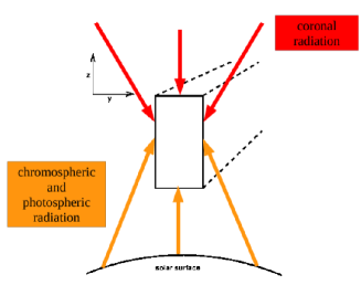
Figure 1: 2D geometrical prominence model: the isolated, isothermal and isobaric slab is standing horizontally above the photosphere. For hydrogen and helium atoms, we consider a chromospheric and photospheric incident radiation coming from below, symmetrically on its sides and bottom. For the helium case, we consider in addition a constant coronal illumination coming from above onto the slab.

In our radiative transfer codes for the hydrogen and helium atoms, we assumed complete redistribution in frequency (CRD).

2.3 Atomic models

We adopted the 5-level plus a continuum hydrogen atom model of Paletou (fp95 (1995)), whose data is consistent with earlier models of Gouttebroze et al. (ghv (1993)).

For neutral helium, we considered two different cases: 19 bound-levels, up to $n=4$, plus a continuum, with no atomic fine structure (hereafter our Hen4 model), or 17 bound-levels, up to $n=3$, plus a continuum, with the atomic fine structure of $2^{3}P$, $3^{3}P$ and $3^{3}D$ levels (hereafter, our Hen3sf model).

Energy levels and statistical weights were taken from the NIST database (Ralchenko et al. nist (2008)). All other atomic data are consistent with those of LG01: effective collision strengths, collisional ionization coefficients and spontaneous emission coefficients are from Benjamin et al. (ben (1999)), collision strengths not defined there are from Benson & Kulander (bk (1972)), and photoionization cross sections are from TOPbase (Fernley et al fernley (1987)).

Our radiative transfer code can explicitely consider collisional rates among them and to/from all fine structure sublevels. For our Hen3sf model, we set to 0 the rates between sublevels of the same level. Otherwise, we used, for each sub-level, the rates given by the later authors even though they were summed over the fine structure. We are aware of this inconsistency which may have only a very small influence on the results exposed hereafter.

Chromospheric illumination for all radiative transitions were taken from Heasley et al. (heasley (1974)), with some additional details which can be found in Labrosse et al. (lg07 (2007)). Coronal illumination for UV lines and continua were taken from Tobiska (tobi (1991)) and Walhstrøm & Carlsson (wc (1994)).

3 Preliminary results

As a first step, results obtained with our 2D radiative transfer code for the hydrogen atom are in very good agreement with those of Heasley & Milkey (hm83 (1983)), Gouttebroze et al. (ghv (1993)) and Paletou (fp95 (1995)).

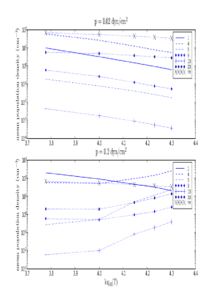
Figure 2: Mean population and electron densities as a function of temperature for two pressures, $p_{g}=0.02$ (top) and $0.2$ (bottom) $\mathrm{dyn}\,\mathrm{cm}^{-2}$. Numbers in the upper-right frames refer to the energy level as follows: 1 for the ground state of He i and 20 the ground state of He ii. The mean population densities for these two levels, as well as for the electron density, are divided by $10^{8}$. The other codes for levels are: 4 for $2^{3}P$, 5 for $2^{1}P$, 9 for $3^{3}D$ and 10 for $3^{1}D$.

As a second step, we have compared the results obtained with our upgraded 2D radiative transfer code for the helium atom with those of LG01, as these last authors have made comprehensive comparisons with the pionneering works of Heasley et al. (heasley (1974)) and Heasley & Milkey (hm78 (1978)). In order to do so, we have used our Hen4 model, without atomic fine structure. Also, their radiative code is 1D plane parallel so that they have neither coronal illumination on the top surface, nor dilution effects varying with the altitude, as in 2D. However, their helium atomic model is more detailed than ours, with 29 bound-levels up to $n\,=\,5$ for He i, 4 bound-levels for He ii, and He iii. Unlike us, they also take into account PRD for the resonance lines H i Ly$\alpha$ and Ly$\beta$, He i $\lambda 584$ Å  and He ii $\lambda 304$ Å.

We have modeled a 2D prominence with $D_{z}\,=\,100\,000$ km and $D_{y}\,=\,1\,000$ km. Its temperature, $T$, could take the respective values: $6\,000$, $10\,000$, $14\,000$, $17\,000$ and $20\,000$ K, and the gas pressure $p_{g}$ could take 2 values: $0.02$ and $0.2\,\mathrm{dyn\,cm^{-2}}$. The microturbulent velocity was fixed at $\xi=5\,\mathrm{km}\,\mathrm{s}^{-1}$. The bottom of the slab was set at $H_{0}=10\,000$ km above the solar surface. We have chosen a 2D spatial grid with $123\times 123$ logarithmically spaced points. We have also used Doppler profiles monotonically sampled with a 0.1 step in Doppler width units.

In Fig. 2, mean population densities variations against temperature are displayed. Mean densities are defined here as:

$$N_{i}\,=\,\displaystyle{\frac{\int_{0}^{D_{y}}\,n_{i}(y,D_{z}/2)dy}{D_{y}}}\,,$$

where $n_{i}(y,D_{z}/2)$ is level $i$ population at the position $y$ at mid-height of the slab ($z=D_{z}/2$). We have focused on the populations of 5 energy levels of He i: $1s^{2}$, $2^{3}P$, $2^{1}P$, $3^{3}D$, $3^{1}D$ labelled 1, 4, 5, 9 et 10, and the ground state of He ii labelled 20. For the sake of clarity, mean population densities of the ground states of He i and He ii, as well as the electron density, are divided by $10^{8}$ on the figure.

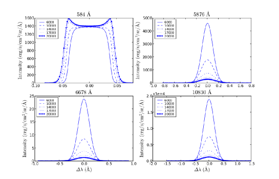
Figure 3: Emergent intensities for lines He i $\lambda 584$ Å, $\lambda 5876$ Å, $\lambda 6678$ Å  and $\lambda 10830$ Å, for a pressure $p_{g}=0.02\,\mathrm{dyn}\,\mathrm{cm}^{-2}$, for 5 different temperatures, and for $D_{z}\,=\,100\,000$ km and $D_{y}\,=\,1\,000$ km. These intensities are computed at slab mid-height, $z=D_{z}/2$, for a line-of-sight perpendicular to the slab.

Figure 4: Same as Fig. 3 for a vertical geometrical extension $D_{z}\,=\,10\,000$ km.

In the low pressure regime, $p_{g}\,=\,0.02\,\mathrm{dyn\,cm^{-2}}$, we recover the same general behaviour as the one shown by in LG01: an increase in temperature reduces the neutral helium mean population and increases the ionized helium mean population, until the latter becomes greater than the former. This transition temperature is around $8\,000$ K for our model, whereas it is $11\,000$ K in LG01. This is explained by PRD effects, as LG01 models in CRD give the same result as ours (N. Labrosse, private communication).

For larger pressures, $p_{g}\,=\,0.2\,\mathrm{dyn\,cm^{-2}}$, it is shown in Fig. 2 that all mean population densities increase with temperature but the ground state of He i. As emphasized indeed by LG01, the helium ionization is less important than in the low pressure case, because of the optical thickness of the helium continuum which prevents incident radiation from reaching the core of the slab. We also recover this effect using our 2D code, when the vertical extension of the slab is made large enough, mimicking a 1D vertical slab model though.

We could also check a posteriori, comparing n(He ii) and n_e, that the assumption that He is not an electron donor remains valid for most of the range of parameters we used. It becomes however questionable for both high pressure and high temperature cases, as shown in Fig. 2.

In Fig. 3, emergent intensities for lines He i $\lambda 584$ Å, $\lambda 5876$ Å, $\lambda 6678$ Å  and $\lambda 10830$ Å  are displayed for a vertical extension $D_{z}=100\,000$ km, for a pressure $p_{g}=0.02\,\mathrm{dyn\,cm^{-2}}$ and for five different temperatures. Intensities are computed at mid-height of the slab, at $z=D_{z}/2$, and for a line-of-sight (los) perpendicular to it.

The general behaviour of these intensities with temperature is in excellent agreement with results presented by LG01 (see e.g., their Fig. 8). Our values for the intensity of the resonance line He i $\lambda 584$ Å are smaller than those of LG01, whereas they are greater for the optically thin $\lambda 5876$ Å  and $\lambda 6678$ Å  lines. This could be explained by PRD effects which play an important role in determining the shape of the resonance line He i $\lambda 584$ Å  as well as in the He i levels 1 and 4 populations. These PRD effects have consequently an impact on the line He i $\lambda 5876$ Å  as its lower level is the level 4, and on ionization via the neutral helium continuum $\lambda 504$ Å. The ground state of He ii mean population density is smaller in LG01. As the triplet levels are populated through the PR mechanism (see Andretta & Jones andretta (1997) and references therein) from the ground state of He ii, our $D_{3}$ multiplet emergent intensity is greater than the ones of LG01.

In Fig. 4, the same emergent intensities are displayed for a smaller vertical extension of $D_{z}\,=\,10\,000$ km (note also that we used, in both case, the same fixed dilution factor for the incident radiation, in order to put in evidence the only effects due to different vertical slab extensions). Emergent intensity values are larger, with relative differences ranging between 15 and 40%, than those displayed in Fig. 3. This shows that significant 2D geometrical effects take place when one reduces the geometrical extension of the slab, and how they impact the magnitude of emergent intensities. Such kind of effects were first put in evidence on H$\alpha$ by Paletou (fp97 (1997)).

4 A realistic spectral synthesis of He i multiplets

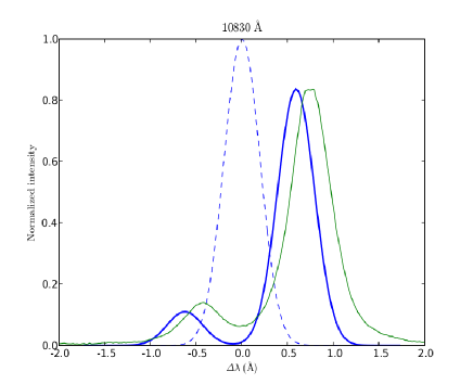
Figure 5: Normalized emergent intensities for the He i $\lambda 10830$ Å  multiplet obtained with the Hen4 atomic model (dashed lines), with the Hen3sf atomic model (thick line), and from THéMIS observations of June 2007, vs. the wavelength shift with respect to the multiplet central (vacuum) wavelength defined as $\lambda=10832.7$ Å. Synthetic profiles are for a line-of-sight perpendicular to the slab. Both the fine-structured and the observed profiles were normalized to the maximum amplitude of the Hen4 synthetic profile. The observed one was also slightly shifted in frequency, for the sake of comparison with the Hen3sf one.

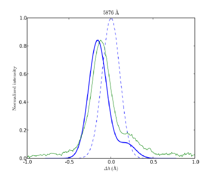
Figure 6: Same as Fig. 5 for the He i $D_{3}$ multiplet whose central (vacuum) wavelength is $5877.4$ Å.

We now focus on He i $D_{3}$ and $\lambda 10830$ Å  multiplets, as our primary aim is to model realistic emergent line profiles consistent with high-resolution spectropolarimetric observations made at the solar telescope THéMIS (see e.g., Paletou et al. fp01 (2001)). With such an instrument, the two “red” and “blue” peaks are, indeed, clearly resolved (see also e.g., Merenda et al. laura (2006), Trujillo Bueno et al. jtb02 (2002), for data taken at the German VTT with the TIP polarimeter, in the near-infrared).

Hereafter, we shall use in our 2D radiative transfer code the Hen3sf atomic model which takes into account the atomic fine structure for the $2^{3}P$, $3^{3}P$ and $3^{3}D$ levels of He i.

4.1 Single slab models

We have modeled a 2D isobaric, isothermic and static prominence with a vertical extension $D_{z}=30\,000$ km and a horizontal extension $D_{y}=5\,000$ km. Its temperature is $T=8\,000$ K, and the gas pressure is $p_{g}=0.05\,\mathrm{dyn\,cm^{-2}}$ which are rather typical values for the modelling of quiescent prominences (see e.g., Gouttebroze et al. ghv (1993)). The microturbulent velocity is $\xi=5\,\mathrm{km}\,\mathrm{s}^{-1}$. The bottom of the slab is set at $H_{0}=10\,000$ km above the solar surface. We have chosen a 2D spatial grid with 243 x 243 logarithmically spaced points.

In Figs. 5 and 6, emergent intensities for He i $\lambda 10830$ Å  and $D_{3}$ multiplets are displayed. They were computed at the slab mid-height, $z=D_{z}/2$, for a los perpendicular to the slab, and the specific intensity was normalized to the maximum value obtained with model Hen4. Then, maximum intensity values are $21871\,\mathrm{erg\,s^{-1}\,cm^{-2}\,sr^{-1}\,}$Å^-1 for the $\lambda 10830$ Å  multiplet and $6473\,\mathrm{erg\,s^{-1}\,cm^{-2}\,sr^{-1}\,}$Å^-1 for the $D_{3}$ multiplet. Taking into account the atomic fine structure, we obtain indeed, 2D emergent line profiles which are directly comparable to high-resolution spectroscopic observations, characterized by two well-resolved subcomponents.

We define $I_{r}$ as the ratio between the intensity of the largest subcomponent peak and the intensity of the smaller peak, that is, $I_{blue}/I_{red}$ for the $D_{3}$ multiplet and $I_{red}/I_{blue}$ for the $\lambda 10830$ Å  multiplet. We remind here that, when the He i $D_{3}$ multiplet becomes optically thick, the $I_{r}$ ratio is lower than 8 (House & Smartt house (1982), Landi Degl’Innocenti landi (1982)). Furthermore, statistics made on this ratio give a mean value of 6 (López Ariste & Casini lopez (2002)), which is not consistent with the commonly used hypothesis that the $D_{3}$ multiplet is optically thin.

We can evaluate the optical thickness of the two multiplets obtained with our 2D model. At the slab mid-height, $z=D_{z}/2$, and for the frequency corresponding to the maximum intensity value:

$$\tau(10830) = 5,1\,\times\,10^{-2}$$

$$\tau(D_{3}) = 4,4\,\times\,10^{-3}\,.$$

The two multiplets are thus optically thin, and we also find that $\tau(10830)\,\sim\,10\,\times\,\tau(D_{3})$, as pointed out by Andretta & Jones (andretta (1997)). In these two cases, $I_{r}$ ratios are indeed around 8.

Having performed several tests with temperatures varying from $6\,000$ to $20\,000$ K and for gas pressures ranging from $0.02$ to $0.2\,\mathrm{dyn}\,\mathrm{cm}^{-2}$, we found that the two multiplets are optically thicker for both high pressure and high temperature atmospheres. However, even in these regimes, the optical thicknesses of the $D_{3}$ multiplet never go beyond $\tau\,\sim\,0.1$. These results are also in accordance with 1D models of Labrosse & Gouttebroze (lg04 (2004)). For instance, these authors found no model for which the $D_{3}$ multiplet is optically thick, and $\tau(10830)>1$ for models where $T>20\,000$ K and $p_{g}>0.64\,\mathrm{dyn}\,\mathrm{cm}^{-2}$ i.e., conditions which are not representative of those expected in quiescent prominences.

Which kind of model could reproduce the observed ratio between subcomponents of the 557.6 and 1083. nm multiplets of He i?

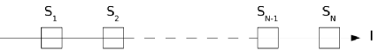
Figure 7: A sketch of the 2D multi-thread prominence model we have adopted. Individual threads are superimposed along the line-of-sight, and there is no radiative interaction between them. Emergent intensities are computed as formal solutions of the radiative transfer equation along a line-of-sight perpendicular to the threads vertical extension, in order to take into account the contribution of each individual thread.

4.2 2D multi-thread models

We have thus decided to model prominences differently, using the fact that they are made of small-scale threads. This is supported both by observations (e.g., Berger et al. berger (2008), Lin et al. lin (2005)) and by MHD simulations (e.g., Low & Petrie low (2005)). The effect of an increased penetration of the incident radiation, using multiple layer modelling, was also shown in 1D by Gouttebroze et al. (goutte02 (2002)). Also, such a 2D non-LTE spatial fine-structure radiative modelling of solar prominences was recently used by Gunár et al. (2007), for the purpose of interpreting UV observations of the Lyman series of hydrogen made with the SUMER spectrograph on-board SoHO.

Hereafter, all the 2D threads (see Fig. 7) are supposed to be identical and located at the same altitude, with similar horizontal and vertical extensions $D_{y}=D_{z}=1\,200$ km which corresponds to a $\approx 1.5$ arcsec angular resolution compatible with what can be decently achieved while doing spectropolarimetry of prominences using ground-based observatories. Such a choice can obvisouly be debated, and we could have considered (much) smaller threads, beyond spatial resolution (see e.g., Vial vial06 (2006), Heinzel ph07 (2007)). However, we leave more detailed investigations about such an issue to further studies.

We considered also that there is no radiative interaction between individual threads. Thus, as a first step, we applied our 2D radiative transfer code for one individual thread. Then we computed emergent intensities as the formal solution of the radiative transfer equation along a los perpendicular to each thread’s vertical extension, in order to take into account the contribution of a bunch of threads. Therefore, the total optical thickness along the los is simply the sum of the optical thicknesses of each individual thread.

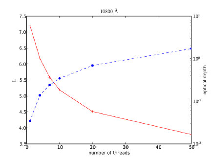
Figure 8: The $I_{r}$ ratio (solid line) and the optical thickness integrated on the slab height (dashed line), for the He i $\lambda 10830$ Å  multiplet versus the number of individual threads, for a gas pressure $p_{g}\,=\,0.5\,\mathrm{dyn}\,\mathrm{cm}^{-2}$ and a temperature $T\,=\,8\,000$ K.

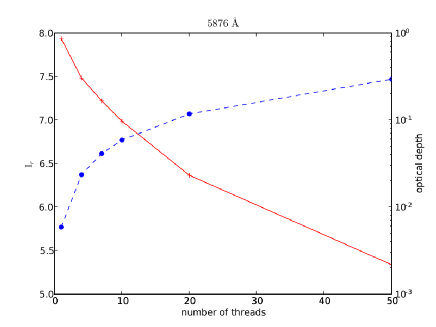
Figure 9: Same as Fig. 8 for the $I_{r}$ ratio and the optical thickness of the He i $D_{3}$ multiplet.

For each (identical) thread, we adopted a gas pressure $p=0.5\,\mathrm{dyn}\,\mathrm{cm}^{-2}$ and a temperature $T=8\,000$ K corresponding to a commonly used temperature for quiescent prominences (see e.g., Engvold et al. engvold (1990), Tandberg-Hanssen tand (1995)).

In Figs. 8 and 9, we have drawn the $I_{r}$ ratio versus the number of threads along the los, for the He i $\lambda 10830$ Å  and $D_{3}$ multiplets. For the calculation of this ratio, we considered the emergent specific intensity integrated over $D_{z}$ as

$${{\bar{I}}(\nu)}\,=\,\displaystyle{\frac{\int_{0}^{D_{z}}\,I(\nu,z)dz}{D_{z}}}\,.$$

The total optical thickness, integrated the same way, is also displayed on the same plots.

We can thus determine the number of threads required, with such models, to obtain a $I_{r}$ ratio around 6 for the He i $D_{3}$ multiplet. In that case, a good value is around 30 threads, which corresponds, however, to a very large total geometrical width of $36\,000$ km for the prominence. The corresponding optical thickness is $\tau(D_{3})\,\sim\,0.2$. For a temperature $T\,=\,17\,000$ K, corresponding to a prominence to corona transition region (PCTR, see e.g., Fontenla et al. fontenlaetal (1996), Anzer & Heinzel anph (1999) and references therein), the number of threads falls to 15, and $\tau(D_{3})\,\sim\,0.7$.

Even though it is still preliminary, yet we favour multi-thread models in order to explain a number of properties of observed He i spectral lines.

However, we are also aware of the fact that, even in a non-magnetic field regime, Stokes $I$ is affected by atomic polarization (R. Casini, private communication). Therefore, a more detailed comparison with spectropolarimetric data would require a more complex treatment of the statistical equilibrium.

5 Conclusion

We have performed here several tests in order to compare our new 2D radiative model against previous works. Results for the hydrogen atom have been compared to Heasley & Milkey (hm83 (1983)), Gouttebroze et al. (ghv (1993)) and Paletou (fp95 (1995)). Results for the helium atom have been mainly compared to Labrosse & Gouttebroze (lg01 (2001), lg04 (2004)). An excellent agreement is reached using our 2D code in the limit of a 1D geometry, with similar atomic models and incident radiation.

We have shown that, taking into account the atomic fine structure for the $2^{3}P$, $3^{3}P$ and $3^{3}D$ levels of He i in our 2D radiative transfer code, allows to compute emergent line profiles which can be directly compared to high-spectral resolution observations. However, using a classical model of isothermal, isobaric, homogeneous and static slabs leads to ratios between the subcomponents of He i $\lambda 10830$ Å  and $D_{3}$ multiplets which do not always support observed values, except for high temperature and high pressure conditions, which are not typical of quiescent prominences (Engvold et al. engvold (1990)).

This led us to undertake a preliminary investigation of 2D multi-thread modelling. It has indeed given us good hints about how it should be possible to reproduce observed characteristics of the $D_{3}$ and $\lambda 10830$ Å  multiplets of He i, such as the ratio between the intensity of their two subcomponents.

Our 2D radiative model will now be more intensively used, taking into account smaller threads, eventually beyond spatial resolution (see Heinzel ph07 (2007) for a recent review) and the radiative interaction between them (e.g., Heinzel ph89 (1989)). We should also include a PCTR for each individual thread in our model, since its influence on hydrogen lines have already been evaluated.

We finally anticipate that our results will be very valuable for the analysis of data coming from a variety of spaceborne (e.g., SoHO, Hinode) and groud-based telescopes such as THéMIS.

- (1) Andretta, V. & Jones, H.P. 1997, ApJ, 489, 375
- (2) Anzer, U. & Heinzel, P. 1999, A&A, 349, 974
- (3) Benjamin, R.A., Skillman, E.D. & Smits, D.P. 1999, ApJ, 514, 307
- (4) Benson, R.S. & Kulander, J.L. 1972, Sol. Phys., 27, 305
- (5) Berger, T.E., Shine, R.A., Slater, G.L., Tarbell, T.D., Title, A.M. et al. 2008, ApJ, 676, L89
- (6) Bommier, V. 1977, Thèse de Doctorat de 3ème cycle, Univ. de Paris VI
- (7) Engvold, O., Hirayama, T., Leroy, J.-L., Priest, E.R. & Tandberg-Hanssen, E. 1990, in Lecture Notes in Physics 363, Dynamics of Quiescent Prominences, eds. V. Ruždjak & E. Tandberg-Hanssen, (New-York: Springer-Verlag), 294
- (8) Fernley, J.A., Seaton, M.J. & Taylor, K.T. 1987, J. Phys. B, 20, 6457
- (9) Fontenla, J.M., Rovira, M., Vial, J.-C. & Gouttebroze, P. 1996, ApJ, 466, 511
- (10) Gopalswamy, N., Mikić, Z., Maia, D., Alexander, H., Cremades, H. et al., 2006, Space Science Reviews, 123, 303
- (11) Gouttebroze, P., Heinzel, P. & Vial, J.-C. 1993, A&AS, 99, 513
- (12) Gouttebroze, P., Labrosse, N., Heinzel, P. & Vial, J.-C. 2002, ESA-SP 505, 421
- (13) Gunár, S., Heinzel, P., Schmieder, B., Schwartz, P. & Anzer, U. 2007, A&A, 472, 929
- (14) Heasley, J.N. & Milkey, R.W. 1978, ApJ, 221, 677
- (15) Heasley, J.N. & Milkey, R.W. 1983, ApJ, 268, 398
- (16) Heasley, J.N., Mihalas, D. & Poland, A.I. 1974, ApJ, 192, 181
- (17) Heinzel, P. 1989, Hvar Obs. Bull., 13(1), 317
- (18) Heinzel, P. 1995, A&A, 299, 563
- (19) Heinzel, P. 2007, in ASP Conf. Ser. 368, The Physics of Chromospheric Plasmas, eds. P. Heinzel, I. Dorotovič & R.J. Rutten (San Francisco: Astronomical Society of the Pacific), 271
- (20) House, L.L. & Smartt, R.N. 1982, Sol. Phys., 80, 53
- (21) Labrosse, N. & Gouttebroze, P. 2001, A&A, 380, 323
- (22) Labrosse, N. & Gouttebroze, P. 2004, ApJ, 617, 614
- (23) Labrosse, N., Gouttebroze, P. & Vial, J.-C. 2007, A&A, 463, 1171
- (24) Landi Degl’Innocenti, E. 1982, Sol. Phys., 79, 291
- (25) Léger, L., Chevallier, L. & Paletou, F. 2007, A&A, 470, 1
- (26) Lin, Y., Engvold, O., Rouppe van der Voort, L.H.M., Wiik, J.E. & Berger, T.E. 2005, Sol. Phys., 226, 239
- (27) López Ariste, A. & Casini, R. 2002, ApJ, 575, 529
- (28) Low, B.C. & Petrie, G.J.D. 2005, ApJ, 626, 551
- (29) Mauas, P.J.D., Andretta, V., Falchi, A., Falciani, R., Teriaca, L. et al. 2005, ApJ, 619, 604
- (30) Merenda, L., Trujillo Bueno, J., Landi Degl’Innocenti, E. & Collados, M. 2006, ApJ, 642, 544
- (31) Paletou, F. 1995, A&A, 302, 587
- (32) Paletou, F. 1996, A&A, 311, 708
- (33) Paletou, F. 1997, A&A, 317, 244
- (34) Paletou, F. & Aulanier, G. 2003, in ASP Conf. Ser. 307, Solar Polarization Workshop 3, eds. J.Trujillo Bueno & J. Sánchez Almeida (San Francisco: Astronomical Society of the Pacific) 458
- (35) Paletou, F. & Léger, L. 2007, JQSRT, 103, 57
- (36) Paletou, F., López Ariste, A., Bommier, V. & Semel, M. 2001, A&A, 375, 39
- (37) Ralchenko Yu., Kramida, A.E., Reader, J. and NIST ASD Team 2008, NIST Atomic Spectra Database (version 3.1.5), available online: http://physics.nist.gov/asd3, National Institute of Standards and Technology, Gaithersburg, MD (USA)
- (38) Rybicki, G.B. & Hummer, D.G. 1992, A&A, 262, 209
- (39) Tandberg-Hanssen, E. 1995, The Nature of Solar Prominences (Dordrecht: Kluwer)
- (40) Tobiska, W.K. 1991, J. Atmos. Terr. Phys., 53, 1005
- (41) Trujillo Bueno, J., Landi Degl’Innocenti, E., Collados, M., Merenda, L. & Manso Sainz, R. 2002, Nature, 415, 403
- (42) Vial, J.-C. 1982, ApJ, 254, 780
- (43) Vial, J.-C. 2006, ESA SP-617, 163
- (44) Vial, J.-C., Rovira, M., Fontenla, J.M. & Gouttebroze, P. 1989, Hvar Obs. Bull., 13(1), 347
- (45) Walhstrøm, C. & Carlsson, M. 1994, ApJ, 433, 417