SUB-WAVELENGTH RESOLUTION IMAGING OF THE SOLAR DEEP INTERIOR

Abstract

We derive expectations for signatures in the measured travel times of waves that interact with thermal anomalies and jets. A series of numerical experiments that involve the dynamic linear evolution of an acoustic wave field in a solar-like stratified spherical shell in the presence of fully 3D time-stationary perturbations are performed. The imprints of these interactions are observed as shifts in wave travel times, which are extracted from these data through methods of time-distance helioseismology (Duvall et al., 1993). In situations where at least one of the spatial dimensions of the scatterer was smaller than a wavelength, oscillatory time shift signals were recovered from the analyses, pointing directly to a means of resolving sub-wavelength features. As evidence for this claim, we present analyses of simulations with spatially localized jets and sound-speed perturbations. We analyze 1 years’ worth solar observations to estimate the noise level associated with the time differences. Based on theoretical estimates, Fresnel zone time shifts associated with the (possible) sharp rotation gradient at the base of the convection zone are of the order 0.01 - 0.1 s, well below the noise level that could be reached with the currently available amount of data ($\sim 0.15-0.2$ s with 10 yrs of data).

1 INTRODUCTION

The deep interior of the Sun holds many a secret in its opaque clutch. Our current understanding of the properties of these regions comes predominantly from the application of methods of global helioseismology to observations of solar oscillations (for reviews, see e.g. Christensen-Dalsgaard, 2002; Christensen-Dalsgaard et al., 2003). However, many aspects of the internal structure and dynamics of the Sun are non-global in nature and may therefore benefit from investigations via techniques of local helioseismology (see review by Gizon & Birch, 2005). Small persistent jets and thermal anomalies in the convection zone, radial variations in the rotation rate at the bottom of the convection zone, convective flows in the interior etc. are examples of such spatially localized phenomena.

A stumbling block associated with seismic studies of the deep interior is the substantial wavelength that propagating $p$ modes attain in this region. At the bottom of the convection zone, the acoustic wavelength is approximately 30 times larger than at the photosphere; a 4 mHz wave with wavelength 2 Mm at the photosphere attains a size of 58 Mm, $\sim 8$% of the solar radius by the time it reaches said bottom. The classical imaging resolution limit of waves with wavelength $\lambda$ is $\lambda/2$, and in practice, more like $\lambda$. This places severe restrictions on our ability to infer properties of the deep interior of the Sun. In the field of optical and acoustic tomography, this resolution limit has been overcome by recognizing that present in the near field of a scatterer is a collection of evanescent waves that contain information about its sub-wavelength structure (e.g. Maynard et al., 1985; Bozhevolnyi & Vohnsen, 1996). That this principle has an analog in the solar case has been theoretically discussed (Bogdan & Cally, 1995; Hanasoge et al., 2008) but conclusive observations of this envelope of evanescent modes are still lacking. And since we are unable to directly observe the bottom of the convection zone, there seems little hope in being able to utilize the near-field signal. Moreover it is not clear how significant a role these evanescent waves play.

The interactions of $p$ modes with localized spatial anomalies in the backdrop of a solar-like stratified medium and the resultant changes in wave travel times are well understood in a range of situations (e.g. Birch & Kosovichev, 2000; Gizon & Birch, 2002). Theory and observation have shown that sub-wavelength sized scatterers can cause significant and observable oscillations in the time shifts (Duvall et al., 2006) and global mode frequencies (e.g. Christensen-Dalsgaard et al., 1995). Moreover, from the work of Birch & Kosovichev (2000), it is clear that the stratification is one of the causes of complex interference patterns that contributes to the oscillations (Fresnel zones) in the travel times. Another participating factor is the limited chromatic extent (25 - 40% of a decade) of the solar wave spectrum; highly bandlimited wave packets are known to produce striking interference patterns because of the emergence of a unique interference length scale (the wavelength).

Wave interactions in local helioseismology are primarily characterized using approximations in the ray, Rytov, or Born limits. One situation wherein the ray approximation is accurate is when the wavelength is much smaller than the characteristic spatial size of the perturbation. This requirement invalidates the ray approximation for a large fraction of deep interior studies. As for the Born approximation, Gizon et al. (2006) have theoretically shown in the context of thin flux tubes that it may break down in the limit of vanishing flux tube radius to imaging wavelength ratio. Thus, extremely small scatterers (at least in the case of magnetic fields and possibly other perturbations) are not well described by the Born limit. Therefore, imaging sub-wavelength aspects of the deep interior using interpretations derived from the Born approximation may also not be very accurate.

Numerical simulations of the solar wave field in full 3D spherical geometry (Hanasoge et al., 2006) provide a means of addressing the wide variety of interaction phenomena described above in a consistent manner. The methods of realization noise subtraction (Hanasoge et al., 2007a) and deep-focusing time-distance helioseismology (Duvall, 2003) are applied in the analysis of the simulation data. In $\S$2, we discuss the numerical methodology and the sound-speed perturbations studied here. We discuss the deep-focusing geometry and time-distance methods and present results from these calculations. The appearance of Fresnel zones in analyses of simulations containing jets at the base of the convection zone is discussed in $\S$3. From time-distance analyses of observations, we attempt in $\S$4 to search for oscillatory time shifts arising as a consequence of the possibly sharp rotation gradient at the base of the convection zone. Finally, we summarize and conclude in $\S$5.

2 Simulations and test cases

The numerical code developed in Hanasoge et al. (2006) and Hanasoge (2007) is the starting point for the results presented herein. The linearized Euler equations in spherical geometry are spatio-temporally evolved in a spherical shell extending from $r=0.24R_{\odot}$ to $1.002R_{\odot}$, where $R_{\odot}$ is the radius of the Sun. Spatial derivatives are calculated using spherical harmonic representations in the horizontal directions while sixth-order accurate compact finite differences (Lele, 1992) are implemented in the radial direction. Temporal evolution is achieved through the repeated application of an optimized second-order accurate Runge-Kutta scheme (Hu et al., 1996). The boundaries are rendered absorbent through the application of boundary conditions prescribed by Thompson (1990) in conjunction with damping sponges placed adjacent to the lower and upper radial boundaries. Waves are excited by a phenomenological forcing term in the radial momentum equation (dipolar sources). The source function is computed in spectral space ($l,m,\omega$) as a set of Gaussian-distributed random numbers for each Fourier component, multiplied by a frequency envelope so as to mimic the solar-like wave power distribution in frequency. Note that $(l,m)$ are the spherical harmonic indices while $\omega$ is the angular frequency. The radial component of the oscillation velocity is extracted at a height of 200 km above the photosphere at each minute. Since the near-surface layers of the Sun are highly convectively unstable, we use the artificially stabilized version described in Hanasoge (2007) (and hence different from standard models of the Sun, e.g. Christensen-Dalsgaard et al. 1996).

An example power spectrum from a simulation is displayed in Figure 1. Because we do not incorporate realistic damping, the power distribution as a function of frequency peaks at approximately 4 mHz, higher than the solar power peak, which occurs at 3.5 mHz. A consequence of this is that the wave packets which contribute to the analyses have systematically shorter wavelengths in comparison to the Sun. The simulations may therefore show a greater degree of sensitivity to perturbations in the deep interior. Finally, to complete the description of the recipe, we apply the method of realization noise subtraction (Hanasoge et al., 2007a) in order to afford the ability to accurately study the effects of perturbations on the wave travel times using short temporal simulation windows. Essentially, using identical realizations of the source function, we perform two simulations: a ‘quiet’ one with no perturbations and another with the anomaly of choice. Because the calculation is linear and we use a linear method to extract the travel times (Gizon & Birch, 2002), the signal-to-noise ratio (SNR) of the measurement can be dramatically improved by subtracting the travel times of the quiet data from the perturbed. See Figure 2 for a demonstration of this procedure. As yet, this method is only possible in theory; there is no way of performing this sort of subtraction when dealing with real data.

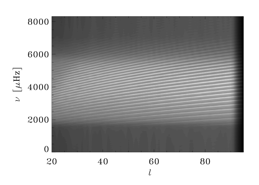
Figure 1: Modal power distribution as a function of frequency ($\nu$) and spherical harmonic degree ($l$) from a 24-hour long simulation with $l_{max}=95$. Standard line of sight Doppler signals are substitued by the radial component of the oscillation velocities, which are extracted at an altitude of 200 km above the photosphere at a cadence of once per minute. The $l\lesssim 20$ modes propagate in proximity of the lower boundary, and are damped out by the damping sponge described in $\S$2, hence not shown here.

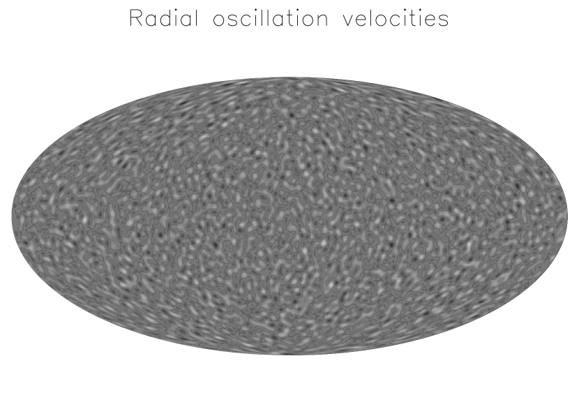
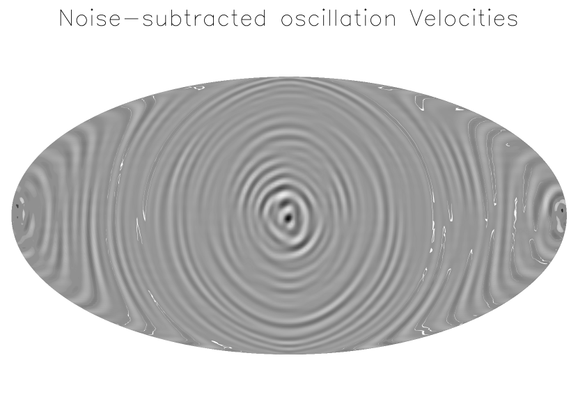
Figure 2: Mollweide projection of the radial oscillation velocities derived from a simulation with a sound-speed perturbation - displayed are raw oscillation data (upper panel) and noise-subtracted velocities (lower panel). The scattering, invisible in the upper panel, becomes far more evident when the realization noise subtraction is performed, i.e. when the velocities of the quiet data are subtracted. This principle also applies to the travel times. Note that the method of noise subtraction is entirely theoretical; no analog exists when dealing with real observations.

2.1 Thermal Anomalies

The existence of a form of thermal asphericity in the tachocline has been suspected for a while now (e.g. Christensen-Dalsgaard et al., 1996). We study here the possibilities relating to the inference of the nature of these deep-interior anomalies. Changes in the thermal structure and hence the sound speed are effected by altering $\Gamma_{1}$, the first adiabatic index, as opposed to perturbations in the pressure or density of the background model which result in hydrostatic inconsistencies and consequently, strong numerical instabilities. Spatially, the perturbations resemble pancakes, thin in the radial direction and broad in the horizontal $(\theta,\phi)$ directions, where $(\theta,\phi)$ denote latitude and longitude respectively. In Figure 3, we show the sound-speed perturbations.

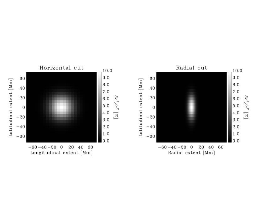
Figure 3: Spatial structure of the sound-speed perturbation. A horizontal and radial cut are displayed. Three cases with the perturbation placed at different radial locations, $r=0.55,0.7,1.0R_{\odot}$ are studied. In all cases, the perturbation is placed at the equator.

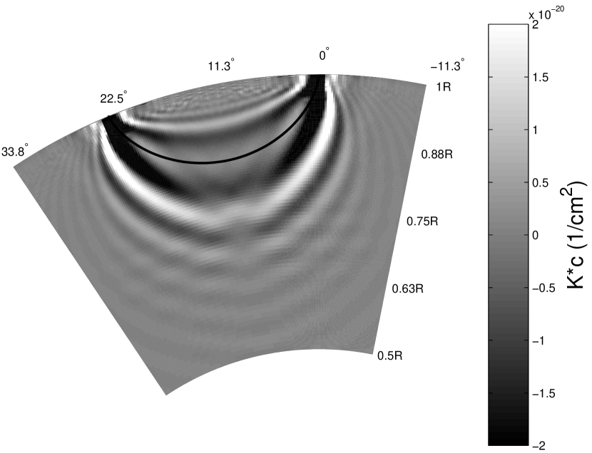
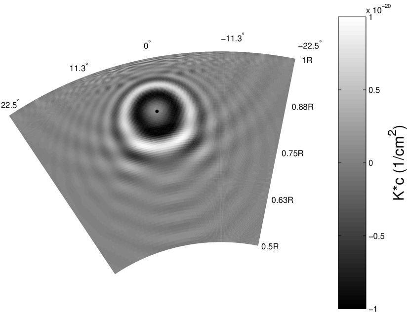
Figure 4: Radial (left panel) and horizontal (right panel) slices of a sound-speed kernel, reproduced from Birch & Kosovichev (2000). A sensitivity kernel is defined as the response as seen in the travel times of a delta-function sized perturbation. In this case, the kernel was computed for the monochromatic frequency of 5 mHz. Complex interference patterns are seen in both slices - provided perturbations are sufficiently small, the alternating signs of the lobes engender oscillating time shifts.

2.2 Time-distance analysis

We use the common midpoint method of analysis (Duvall, 2003) to average the data and extract $p$-mode travel times. Note that we do not perform any form of phase-speed filtering. The analysis proceeds as follows: for a given point $(\theta_{0},\phi_{0})$ and a travel distance at the surface $\Delta$, we search for all points that lie on a circle of diameter $\Delta$ with center $(\theta_{0},\phi_{0})$. Subsequently, we cross correlate signals at points that are located diametrically opposite each other and average these pairwise cross correlations over the circular region. We then fit the averaged cross correlation using the method of Gizon & Birch (2002) to obtain the travel time at the point $\tau(\theta_{0},\phi_{0})$. Since there is no directional bias in the averaging procedure, the quantity $\tau$ is classified as the ‘mean travel time’ and is sensitive primarily to sound-speed anomalies along the ray path.

In Figure 6, we show the time shifts associated with the interactions of the waves with the sound-speed perturbations. It is our understanding that the oscillations seen in the maps are a consequence of the highly sub-wavelength nature of these interactions. The fact that time shifts of both signs are seen, inspite of a solely positive change in the sound speed, is indicative of subtler interference phenomena that are at play. The sensitivity kernels of Birch & Kosovichev (2000) show the appearance of these ‘Fresnel zone’-like structures (see Figure  4), due in part to the complex interference patterns of waves at constant frequency. Duvall et al. (2006) have experimentally recovered the oscillatory travel-time features of these sensitivity kernels that occur when sub-wavelength sized perturbations are encountered.

In Figure 6, the solid lines in the two panels indicate the ray theoretic travel distance for waves whose inner turning point coincides with the radial position of the perturbation. It is seen that waves whose turning points lie well above (shorter travel distance waves) the perturbation seem equally if not more sensitive (due to the proximity of the propagation regions of these waves to the surface) to the perturbation. Evidently, the theoretical picture of waves being sensitive only to perturbations located above their inner turning points is too simplistic to explain this phenomenon. Wave scattering in the Sun is a predominantly linear phenomenon, especially in the deep interior, where the waves and convection are presumably decoupled. Thus the scattering redistributes modal energies across a range of wave numbers, at a fixed frequency. And because we do not phase speed filter this data, the cross correlation for a specific travel distance retains a sensitivity to contributions from scattered waves at different wave numbers (and therefore different travel distances).

The time shifts are measured according to the common mid-point procedure (described above) at a large number of points. The perturbation lies at horizontal co-ordinates $(0,0)$ and as is evident from Figure 3, rotationally symmetric about the center point. Thus, azimuthally averaging the time shifts about $(0,0)$, we are left with two variables (see Figure 5), namely the distance of the point of measurement from the center of the perturbation (x-axis) and the travel distance (y-axis). Having therefore defined the geometry involved in the construction of Figure 6, we are ready to address questions relating to the fringes. Because the radial extent of the perturbation is significantly smaller the wavelength of the acoustic waves at either depth, we must prepare ourselves for the emergence of strong sub-wavelength effects as a function of the travel distance. And indeed, numerous fringes appear in both cases as harbingers of the presence of this sub-wavelength feature. The kernel in Figure 4, which albeit is for a monochromatic wave, contains these oscillating positive and negative signed lobes that hint at the possibility of such effects.

Meanwhile in the horizontal direction, we see some sign switching for the $r=0.55R_{\odot}$ case while not so much for the other. This is because the horizontal size of the perturbation ($\sim 50$ Mm, see Figure 3) is comparable to the wavelength of 58 Mm at $r=0.7R_{\odot}$, while it is decidedly a subwavelength feature when compared to the 70 Mm long waves at $r=0.55R_{\odot}$. As one moves away from the perturbation, these alternating signed lobes are encountered again (Figure 4). Depending on the size of the perturbation, these lobes may end up being averaged, not showing up in the time shifts (size comparable to or greater than the wavelength) or may result in oscillations (size smaller than the wavelength).

Although our knowledge of the structure and dynamics of the tachocline region is limited, it is certainly well within the realm of possibility that there exist thermal asphericities whose dimensions may be smaller than a wavelength. In such a situation, ray theory is untenable, and a wave mechanical description becomes necessary. A prominent source of solar observational data is the Michelson Doppler Imager (MDI; Scherrer et al., 1995) instrument, onboard the Solar and Heliospheric Observatory (SOHO). The MDI medium-$l$ program has approximately 10-yr long line of sight Doppler velocity observations of the solar surface. However, this data is somewhat corrupted by systematics such as strong center-to-limb variations ($\sim$ 6 – 18s) in the zeroth order wave travel time, aliasing across the spatial Nyquist, fore-shortening, line-of-sight projection related effects etc. The resolution of these effects may be in sight (e.g Zhao et al., 2007; Duvall et al., 2008) but the issues are outstanding as yet. Studying the interior thermal structure of the Sun requires the measurement of absolute quantities like the mean travel time, in contrast to investigations of flows which are described by relative quantities like travel-time differences. Absolute quantities are very difficult to pin down precisely because of this center-to-limb variation, sprouting questions like what value of the mean travel time is ‘correct’ and what part is systematic. For some of these reasons, we have not pursued observational investigations of the thermal structure in the deep solar interior. We now turn to studies of jets.

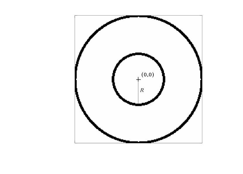
Figure 5: Travel-time averaging geometry. The outer circle represents the observational boundaries of the sphere, while the inner indicates points that are at distance $R$ from the location of the surface projection of the perturbation, $(0,0)$. Each point on the travel-time map is associated with a travel time that is computed by (a) cross correlating signals at points at a distance $\Delta$ with it and (b) fitting the averaged cross correlation by a Gabor wavelet. Within the noise level, we expect identical time shifts at all points along the inner circle due to the (horizontal) directionally unbiased nature of wave scattering by the symmetric thermal anomalies of Figure 3. Thus we may average the time shifts on this annulus to improve the signal-to-noise properties of the analysis; we are then left with two co-ordinates, the travel distance $\Delta$ and distance from the scatterer, $R$, as described in Figure 6.

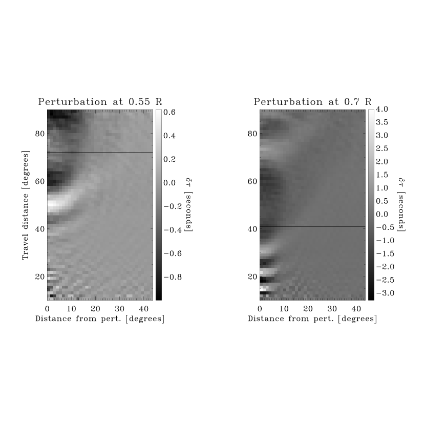
Figure 6: Time shifts caused by localized sound-speed perturbations (see Figure 3) centered at $r=0.55,0.7R_{\odot}$. These shifts are recorded at a series of wave travel distances and at numerous horizontal locations on the surface. Because the perturbation exhibits a horizontal rotational symmetry (see Figure 3) about its center point, we azimuthally average the time shifts around this point. The vertical axis is the travel distance, also the distance between correlation points. The horizontal axis is the angular distance of the measurement point from the horizontal center of the perturbation $(0,0)$. Wavelengths of 4 mHz waves at these depths are approximately 70 and 58 Mm respectively. The radial size of the perturbation is significantly smaller than the wavelength in either case, a manifestion of which are the variations of the time shifts with travel distance. The two horizontal lines show the ray theoretic travel distance for waves whose inner turning point coincides with the radial position of the perturbation. Because the horizontal size of the perturbation is comparable to the wavelength in the $r=0.7R_{\odot}$ case, we do not see a flip in the sign of the time shift as we move horizontally away from the perturbation. It is however visible in the $r=0.55R_{\odot}$, where the sound-speed perturbation is decidedly sub-wavelength in size.

3 Jets in the convection zone

We choose jets with spatial structure of the form displayed in Figure 7. We can no longer apply the straightforward common midpoint analysis of $\S$2.2 because of the inherent directional bias that flows introduce. Waves that move along with flow are sped up and vice versa. Keeping the same geometry as above, i.e. choosing a center point and searching for a set of points at a constant distance away from this point, we then divide up the circle into four sectors: north, south, east, and west. Points on each quadrant are cross correlated with their diametrically opposite counterparts and the averaging is restricted to these quadrants, thus allowing us to study north-south and east-west directed flows in isolation. See Figure 8 for an illustration of this geometry. Time shifts, as before, are computed for a variety of travel distances and at a large number of surface points. Because the jet is invariant over longitude, we average the time shifts over all longitudes, thus leaving us two independent variables, namely the travel distance and latitude.

The difference time shifts (so-called because we take the difference of the travel times) obtained with this averaging scheme are shown in Figure 9. Because of the large horizontal size of the jets, fringe-like time shift oscillations do not appear as the latitudinal distance from the jet grows. The radial extent of jet ($\sim$ 40 Mm) is smaller than the wavelength at $r=0.71R_{\odot}$ (58 Mm) but becomes comparable in the $r=0.81R_{\odot}$ centered case (wavelength of 42 Mm). Thus the time shift fringes are seen in the former but not in the latter.

In the process of discovering these effects related to the sub-wavelength spatial dimensions of scatterers, it was realized that by studying the amplitude of these oscillatory time shifts in comparison to the dominant shift, we could place bounds on the size of the scatterer. In other words, the tachocline thickness, thought by some to be close to a wavelength (e.g. Kosovichev, 1996) and others to be much smaller (e.g. Elliott & Gough, 1999) is then a parameter that can be estimated by this method. Much to our chagrin however, the lack of a sufficient signal-to-noise ratio has blocked our efforts in this regard. This shall be the topic of discussion for the remaining part of this paper.

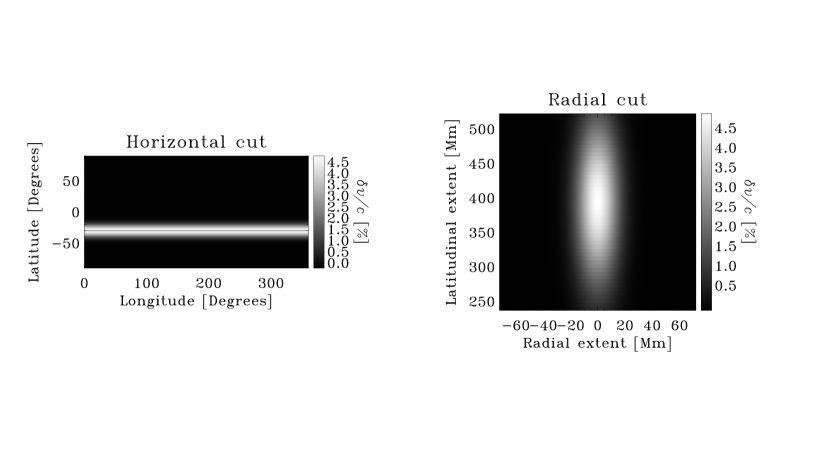
Figure 7: Form of jets used in simulations. The jet structure is highly anisotropic, with large horizontal dimensions but an extremely thin radial extent. The maximum jet velocity is set to 5% of local sound speed, amounting to 11.25 km/s and 8.5 km/s at $r=0.71,0.81R_{\odot}$ respectively. Although the model jet velocities may be unrealistically large, the time shifts may be linearly scaled with the flow velocity, thus allowing us to estimate the expected time shifts for much weaker jets.

Figure 8: Quadrant time-distance averaging geometry used for the study of flows. Points on each quadrant are cross correlated with those diametrically opposite. The east-west quadrants are separated from the north-south so as to study flows in these directions in isolation. For example, the difference time shift $\tau_{e-w}-\tau_{w-e}$ is an indicator of flow magnitude in the east west direction, where $\tau_{e-w}$ is the travel time from a point on the east quadrant to its diametrically opposite counterpart on the west quadrant, and vice-versa for $\tau_{w-e}$.

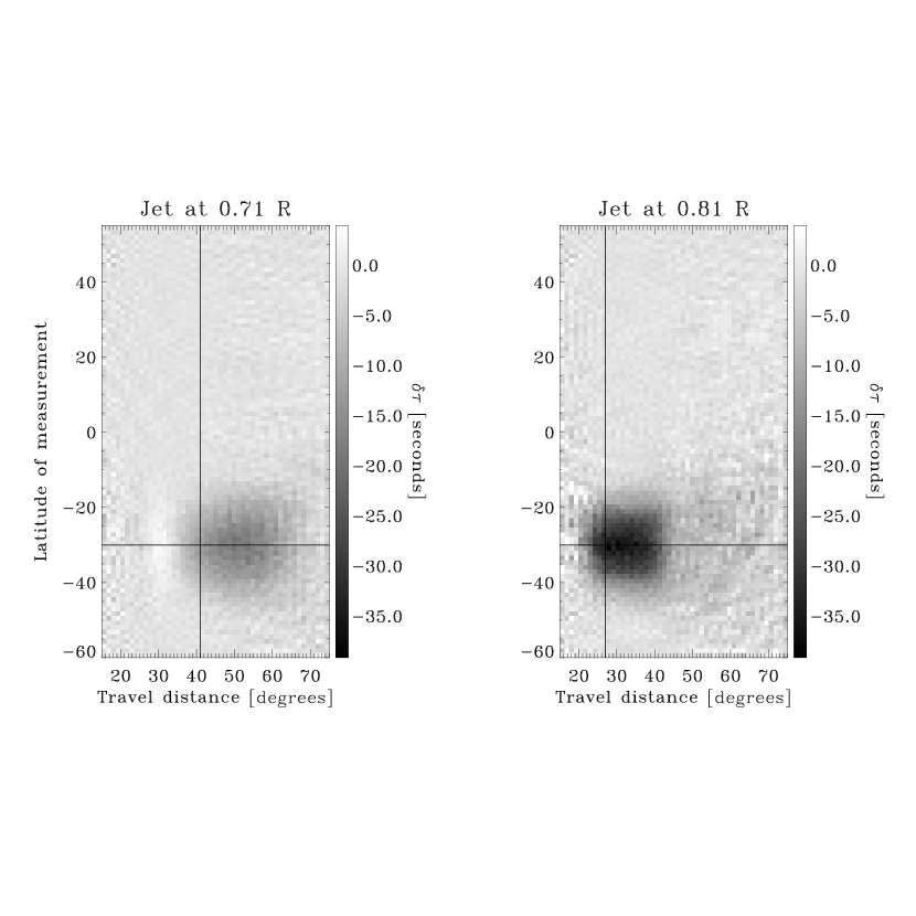
Figure 9: Statistically significant difference time shifts caused by the interaction of waves with jets in the deep interior (see Figure 7). Because the jet is axisymmetric, we average the difference time shifts over all longitudes. The cross-hairs show the center of the jet, i.e. the latitude about which the jet is centered (horizontal line) and the travel distance of a ray whose inner turning point is the radial center of the jet (vertical line). The horizontal extent of the jet is larger than a wavelength, resulting in time shifts of only one sign (as a function of latitude). Radially, it is sub-wavelength in size for the $r=0.71R_{\odot}$ centered jet (wavelength 74 Mm), but comparable to the wavelength for the $r=0.81R_{\odot}$ case (55 Mm long waves), thereby creating weak fringe-like patterns in the time shifts of the former but not so much the latter. The simulation was performed with $l_{max}=95$ and hence the shortest travel distance that could be recovered from the data was approximately $15^{\circ}$.

4 Study of the tachocline

Our initial assessment of the situation was that with a number of years of MDI medium-$l$ observations, a latitudinal band of $\pm 30^{\circ}$ around the equator where differential rotation is nearly absent, we might have enough data to conclude one way or the other about the thickness of the tachocline. Before analyzing observations, we first theoretically investigated the effects of an angular velocity gradient at the base of the convection zone on the travel times. We performed simulations with a velocity perturbation that took the form of a rigidly rotating radiative interior (rotation rate of 9.065 $\mu{\rm Rad}~{}{\rm s}^{-1}$) tied to a non-rotating convection zone. The size of the interface between the rotating and non-rotating zones was varied in order to sharpen/weaken the gradient. With sufficient sharpness, a sub-wavelength sized feature could be created and vice versa. In Figure 10 we display the time shifts recovered from this simulation (the rotation gradient at the interface was $1.1\times 10^{-4}{\rm s}^{-1}$); a Fresnel zone is clearly observed.

As a first step, we analyzed and extracted rotation signals from 1 year of medium-$l$ observations (see Figure 11). The Fresnel zone signals are expected to scale linearly with the rotation gradient at the base of the convection zone. From the rotation inversions of observed frequency splittings (e.g. Schou et al., 1998), we estimate the rotation gradient to be at least $1.44\times 10^{-6}{\rm s}^{-1}$, two orders of magnitude less than the simulated values. The Fresnel zone time shift associated with the solar rotation gradient is possibly 0.01-0.1 seconds or less (the peak modal power occurs at a lower frequency in the Sun than the simulations) in magnitude. Two stumbling blocks lie on the path to the detection of solar Fresnel zones: (1) precisely determining the zeroth order rotation related time shift curve, and (2) achieving high signal-to-noise ratios. While the former presents a somewhat formidable challenge, the latter seems to lie in the realm of impossibility, at least with the current quantity of data available. The error bars in Figure 12 for the one year period appear to be the order of 0.5-0.6 seconds; since the noise goes down as the square root of observational time, we expect a $\sqrt{10}=3.16$ reduction, setting the error bars at around 0.15 - 0.2 seconds. Unfortunately this may well be much larger than the estimated observational effect.

Figure 10: Simulated difference time shifts averaged over the southern latitudes (dotted) and the northern latitides (solid line). The simulated east-west time shifts contain a statistically significant Fresnel zone, seen for waves that travel a distance of $25^{\circ}$ or so (the Fresnel zone disappears when the FWHM becomes comparable to a wavelength). The noise seen at larger distances is presumably from the poor quality of noise subtraction.

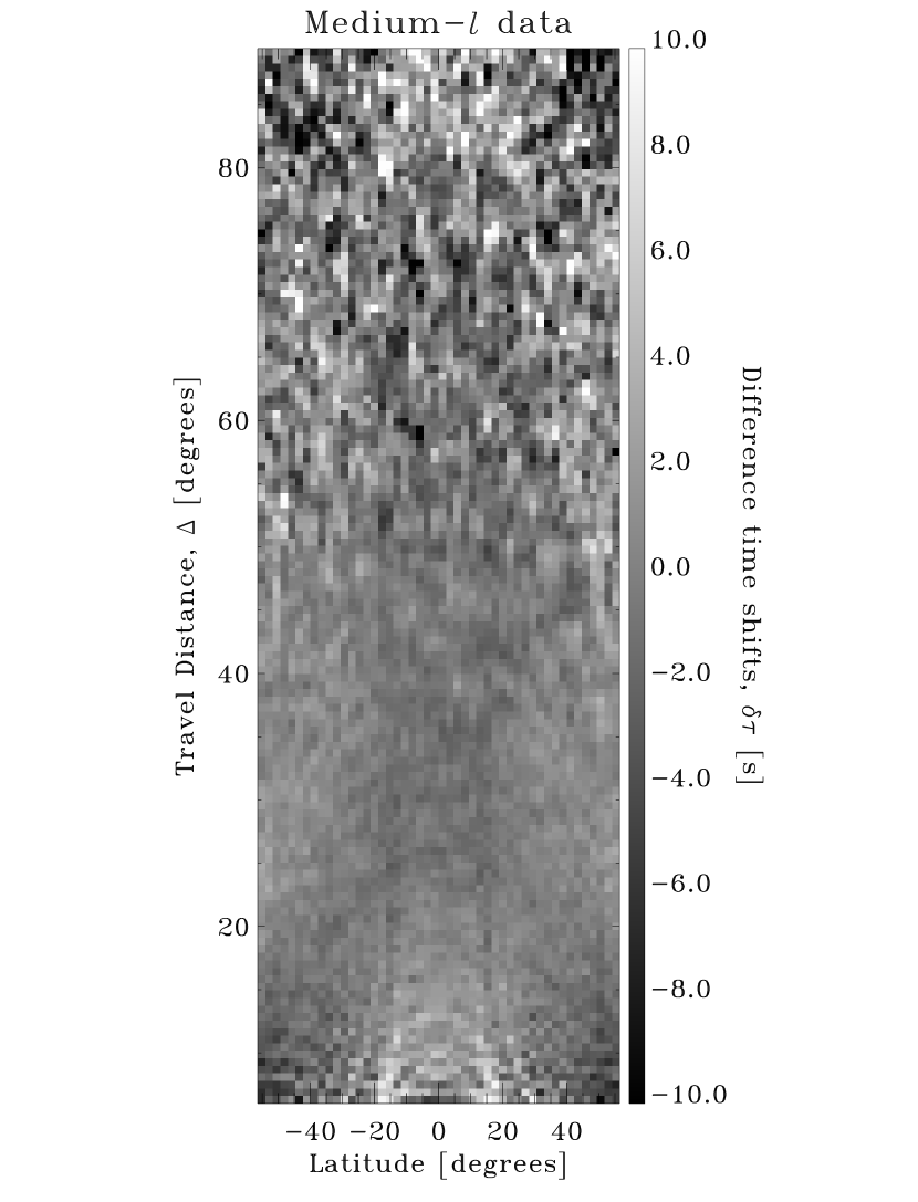
Figure 11: Longitudinally averaged difference time shifts obtained from analyses of 1 year of untracked MDI medium-$l$ observations. Subtle effects such as Fresnel zones are entirely masked by the noise in the travel-time map. A zeroth order rotation related time difference has been subtracted for each distance. This benchmark time was estimated by averaging cross covariances over the entire available disk and fitting the resultant. We believe that the features seen extending over the small distance range are due to systematical issues of unknown origin.

Figure 12: Difference time shifts of Figure 11 averaged over the entire latitude range. Fresnel zones, if any, hide well beneath the noise of the travel-time map, which are indicated by the vertical bars.

5 Conclusions

We have attempted to explore the prospects for the seismology of the solar deep interior through the application of techniques of deep-focusing time-distance helioseismology on numerical simulations and MDI observations. The solar dynamo is possibly closely tied to the dynamics in the tachocline, a remarkably important but relatively poorly understood region. In this regard, any one of the following would be very useful: strong observational constraints on the thickness of the tachocline, inferences of rotational deviants such as jets (Christensen-Dalsgaard et al., 2005), the structure of the thermal anomalies, etc. Azimuthally symmetric features are probably better off being studied using the methods of global helioseismology; however, spatially limited perturbations are perhaps more amenable to the techniques of local helioseismology.

The study of the interactions between waves and sub-wavelength sized perturbations bring to the fore a means of using wave statistical information. We have attempted to exploit the premise that features with sub-wavelength spatial dimensions create Fresnel zones in the difference shifts (while the super-wavelength counterparts do not) in order to place strong constraints on the angular velocity gradient at the bottom of the convection zone.

The prospects? Figure 11 presents an unexciting forecast for local helioseismic investigations of the solar tachocline and the nearby regions. However, encouraging results are derived for studies of the moderately deep convection zone and near-surface regions, which provide reasonable signal-to-noise ratios.

References

- Birch & Kosovichev (2000) Birch, A. C. & Kosovichev, A. G. 2000, ApJ, 192, 193
- Bogdan & Cally (1995) Bogdan, T. J., & Cally, P. S. 1995, ApJ, 453, 919
- Bogdan (1997) Bogdan, T. J. 1997, ApJ, 477, 475
- Bozhevolnyi & Vohnsen (1996) Bozhevolnyi, S. I. & Vohnsen, B. 1996, Physics Review Letters, 77, 3351
- Christensen-Dalsgaard et al. (1995) Christensen-Dalsgaard, J., Monteiro, M. J. P. F. G., & Thompson, M. J. 1995, MNRAS, 276, 283
- Christensen-Dalsgaard et al. (1996) Christensen-Dalsgaard, J., et al. 1996, Science, 272, 1286
- Christensen-Dalsgaard (2002) Christensen-Dalsgaard, J. 2002, RvMP, 74, 1073
- Christensen-Dalsgaard et al. (2003) Christensen-Dalsgaard, J., Thompson, M. J., Miesch, M. S., & Toomre, J. 2003, ARA&A, 41, 599
- Christensen-Dalsgaard et al. (2005) Christensen-Dalsgaard, J. et al. 2005, ASPC, 346, 115
- Couvidat, Birch, & Kosovichev (2006) Couvidat, S., Birch, A. C., & Kosovichev, A. G. 2006, ApJ, 640, 516
- Duvall et al. (1993) Duvall, T. L., Jefferies, S. M., Harvey, J. W., & Pomerantz, M. A. 1993, Nature, 362, 430
- Duvall (2003) Duvall, T. L., Jr. 2003, SOHO 12/GONG+ 2002 proceedings, Ed.: H. Sawaya-Lacoste, ESA Publications Division, 259
- Duvall et al. (2006) Duvall, T. L., Jr., Birch, A. C., & Gizon, L. 2006, ApJ, 646, 553
- Duvall et al. (2008) Duvall, T. L., Jr., Hanasoge, S. M., & Birch, A. C., in prep
- Elliott & Gough (1999) Elliott, J. R. & Gough, D. O. 1999, ApJ, 516, 475
- Gizon & Birch (2002) Gizon, L., & Birch, A. C. 2002, ApJ, 571, 966
- Gizon et al. (2006) Gizon, L., Hanasoge, S. M., & Birch, A. C. 2006, ApJ, 643, 549
- Gizon & Birch (2005) Gizon, L. & Birch, A. C. 2005, Living Reviews in Solar Physics, 2, 6
- Hanasoge et al. (2006) Hanasoge, S. M. et al. 2006, ApJ, 648, 1268
- Hanasoge et al. (2007a) Hanasoge, S. M., Duvall, T. L., Jr., & Couvidat, S. 2007a, ApJ, 664, 1234
- Hanasoge (2007) Hanasoge, S. M. 2007, Ph. D. thesis, Stanford University, http://soi.stanford.edu/papers/dissertations/hanasoge/
- Hanasoge et al. (2008) Hanasoge, S. M., Birch, A. C., Bogdan, T. J., & Gizon, L. 2008, ApJ, 680, 774
- Hu et al. (1996) Hu, F. Q., Hussaini, M. Y., & Manthey, J. L. 1996, Journal of Computational Physics, 124, 177
- Kosovichev (1996) Kosovichev, A. G. 1996, ApJ, 469L, 61
- Kosovichev & Duvall (1997) Kosovichev, A. G. & Duvall, T. L., Jr. 1997, SCORe proceedings, Ed.: F.P. Pijpers, J. Christensen-Dalsgaard, and C.S. Rosenthal, Kluwer Academic Publishers, 241
- Lele (1992) Lele, S. K. 1992, Journal of Computational Physics, 103, 16
- Maynard et al. (1985) Maynard J. D., Williams, E. G., & Lee, Y. 1985, Journal of the Acoustical Society of America, 78, 1395
- Scherrer et al. (1995) Scherrer et al. 1995, Sol. Phys., 162, 129
- Schou et al. (1998) Schou, J. et al. 1998, ApJ, 505, 390
- Thompson (1990) Thompson, K. W. 1990, Journal of Computational Physics, 89, 439
- Zhao et al. (2007) Zhao, J., Hartlep, T., Kosovichev, A. G., & Mansour, N. N. 2007, AGU abstract