Geometric strong segregation theory for compositionally asymmetric diblock copolymer melts

Abstract

We have identified the effect of the Wigner-Seitz cell geometry in the strong segregation limit of diblock copolymer melts with strong composition asymmetry. A variational problem is proposed describing the distortions of the chain paths due to the geometric constraints imposed by the cell shape. We computed the geometric excess energies for cylindrical phases arranged into hexagonal, square, and triangular lattices and explicitly demonstrated that the hexagonal lattice has the lowest energy for a fixed cell area.

Block copolymers are a well-known class of smart materials that can produce a wide variety of complex equilibrium microstructures Bates and Fredrickson (1999); Goodman (1982); Aggarwal (1970); Bates and Fredrickson (1990). Since the late 70’s, these systems have received significant attention by theorists, and many of the copolymer system phases are now well explained on the basis of energy minimization arguments Helfand (1975); Helfand and Wasserman (1976, 1978, 1980); Leibler (1980); Semenov (1985); Ohta and Kawasaki (1986); Likhtman and Semenov (1994); Olmsted and Milner (1998). Further advances in computational techniques allowed studies of the phase behavior in block copolymer systems with the help of direct numerical solution of models which explicitly incorporate statistical mechanics of polymer chains, providing a connection between the observed microstructures and the underlying microscopic material parameters Matsen and Schick (1994); Matsen and Whitmore (1996); Groot and Madden (1998); Murat et al. (1999); Matsen (2001, 2002); Schultz et al. (2002); Cochran et al. (2006); Bosse et al. (2006). More recently, a renewed interest in block copolymer systems was stimulated by the studies of geometrically constrained systems, such as block copolymers confined to the surface of a substrate or the inside of nanopores Lambooy et al. (1994); Knoll et al. (2002); Xiang et al. (2004). Numerical studies of these systems showed a rich variety of microstructures with very intricate geometries Li et al. (2006); Chen et al. (2007); Chantawansri et al. (2007); Yu et al. (2007).

An important regime in which the self-organizing behavior of block copolymer systems becomes especially pronounced is the strong segregation limit, in which monomers of different types segregate almost completely into non-overlapping regions of space. In the case of diblock copolymers, the first theory of the strong segregation limit was proposed by Semenov, who computed the phase coexistence boundaries for several types of microphases with simple geometries Semenov (1985). His results were essentially corroborated by the computational studies of self-consistent mean-field models and extended under a number of simplifying assumptions to include more exotic phases Matsen and Schick (1994); Matsen and Whitmore (1996); Likhtman and Semenov (1994); Olmsted and Milner (1998). Nevertheless, the original Semenov’s theory crucially relies on approximating the Wigner-Seitz cell of the corresponding periodic structure by a disk of the same area in the case of cylindrical phases, or a ball of the same volume in the case of spherical phases. Thus, Semenov’s theory neglects the effect of the cell geometry and, therefore, cannot distinguish between the structures which are characterized by different unit cell types (as, e.g., body-centered cubic versus face-centered cubic lattices of spheres). This point becomes even more critical when considering the effects of confinement, since the domain shape must be truly important in such problems.

In this paper, we propose an extension of the strong segregation theory for block copolymer systems which includes the effect of geometric constraints on the chain configurations. Specifically, we investigate the case of diblock copolymers with strong composition asymmetry, in which most of the “unpleasant” features of the strong segregation limit Matsen (2002) are under control, allowing us to concentrate on essentially the only remaining issue of the effect of the geometry. We formulate a variational problem that gives the excess energy due to geometric factors and, in particular, allows to discriminate between different lattice types with the same unit cell volume in the case of periodic microstructures. To illustrate the latter point, we explicitly compute the excess energies for cylindrical phases on three fundamental two-dimensional lattices and demonstrate that, as intuitively and experimentally expected, the hexagonal lattice has the lowest energy.

Consider a system of linear polymer chains consisting of $N$ monomers of type A bonded covalently with $fN$ monomers of type B, with $f\ll 1$. If each A- and B-monomer has excluded volume $v$, then $f$ is basically the volume fraction of the B-monomer. We introduce the Flory interaction parameter $\chi$, the Kuhn statistical length $b$, and the root-mean-square end-to-end distance $R\simeq b\sqrt{N}$. The confinement domain (or the Wigner-Seitz cell for periodic structures) is denoted by $\Omega\subset\mathbb{R}^{3}$.

In the strong segregation regime $\chi N\gg 1$ the A- and B-monomers locally segregate into disjoint subsets $\Omega_{A}$ and $\Omega_{B}$ of $\Omega$, with a sharply defined interface $\Gamma=\partial\Omega_{A}\cap\partial\Omega_{B}$ containing the A-B junctions. Based on this observation and the Gaussian chain model, Semenov computed the free energy of the system as a sum of three contributions:

$$F=F_{\mathrm{interface}}+F_{\mathrm{core}}+F_{\mathrm{corona}}.$$ (1)

Here, $F_{\mathrm{interface}}$ is the interfacial energy given by

$$F_{\mathrm{interface}}=\sigma\int_{\Gamma}dA,\qquad\sigma=\frac{\sigma_{0}k_{B}T\chi^{1/2}b}{v},$$ (2)

where $\sigma_{0}$ is a dimensionless parameter of order 1, $k_{B}$ is the Boltzmann constant and $T$ is temperature. Next, $F_{\mathrm{core}}$ is the energy of the small B-monomer core, assumed to be radially symmetric Semenov (1985); Likhtman and Semenov (1994); Matsen (2002):

$$F_{\mathrm{core}}=\frac{3\pi^{2}k_{B}T}{8vN^{2}b^{2}f^{2}}\int_{\Omega_{B}}z^{2}(\mathbf{r})\,d\mathbf{r},$$ (3)

where $z(\mathbf{r})$ is the distance from $\mathbf{r}$ to $\Gamma$. Finally, $F_{\mathrm{corona}}$ is the energy of the corona composed of the A-monomers filling $\Omega_{A}$. Both calculations of $F_{\mathrm{core}}$ and $F_{\mathrm{corona}}$ rely on the strongly stretched Gaussian chain assumption. However, the computations differ crucially, since the surface $\Gamma$, as seen from $\Omega_{A}$, is convex, while from the side of $\Omega_{B}$ it is concave. A parabolic brush assumption can be used to compute $F_{\mathrm{core}}$, while one needs to take into account the exclusion zone to compute $F_{\mathrm{corona}}$ Semenov (1985); Ball et al. (1991); Milner (1991); Semenov (1993); Likhtman and Semenov (1994); Belyi (2004); Matsen (2002). In the original Semenov’s theory, the domain $\Omega$ is replaced with a cylindrical or spherical region of the same volume, and the Alexander-de Gennes brush assumption Alexander (1977); de Gennes (1976) is used to compute the energy. This, however, does not affect the leading order contribution to the energy at small volume fractions, since the energy is dominated by the singularity near the interface Semenov (1985); Ball et al. (1991); Semenov (1993); Fredrickson (1993).

We will now compute the corona energy, taking also the geometric effects into account. We start with the self-consistent mean-field theory in which each polymer molecule is treated as a Gaussian chain with the position $\mathbf{r}_{0}\in\Gamma$ of the A-B junction uniformly distributed on the interface (the latter is justified for $f\ll 1$). Then the corona free energy is (up to an additive constant)

$$\frac{F_{\mathrm{corona}}}{k_{B}T}=-\nu\int_{\Gamma}\left(\ln\int_{\Omega_{A}^{N}}e^{-H_{A}/k_{B}T}\prod_{n=1}^{N}d\mathbf{r}_{n}\right)dA.$$ (4)

Here, $\mathbf{r}_{1},\ldots,\mathbf{r}_{N}$ denote the positions of the A-monomers, $\mathbf{r}_{0}$ is the position of the A-B junction, $\nu$ is the density of the A-B junctions on $\Gamma$, and $H_{A}$ is the Gaussian chain Hamiltonian:

$$H_{A} = \frac{3k_{B}T}{2b^{2}}\sum_{n=1}^{N}(\mathbf{r}_{n}-\mathbf{r}_{n-1})^{2}$$ (5)

$$+ \sum_{n=1}^{N}\varphi_{A}(\mathbf{r}_{n})-\frac{\int_{\Omega_{A}}\varphi_{A}(\mathbf{r})d\mathbf{r}}{\nu v\int_{\Gamma}dA},$$

where $\varphi_{A}$ is the self-consistent field (a Lagrange multiplier) enforcing the average monomer density to be $v^{-1}$ everywhere in $\Omega_{A}$.

In the strong segregation limit the chains are highly stretched, i.e. we have $|r_{N}-r_{0}|\gg R_{g}$, so one would naturally want to use the method of steepest descent to evaluate the integral in (4). However, to proceed further we note a general difficulty that in the strong segregation limit the integral in (4) is not dominated by the global minimizer of $H_{A}$, the fluctuations of the end-point positions $\mathbf{r}_{N}$ actively contribute to the free energy of the chains Matsen (2002). Nevertheless, when $\Gamma$ is convex, as seen from $\Omega_{A}$, an exclusion zone must form around $\Omega_{B}$ which is free of the chain ends Semenov (1985); Ball et al. (1991). Moreover, for $f\ll 1$ this exclusion zone must occupy most of $\Omega_{A}$, pushing chain ends close to the cell boundary. In the case when $\Omega$ is a disk an exact solution to the problem shows that the exclusion layer extends to the fraction of $2/\pi\simeq 0.64$ of the disk radius, and in fact the majority of the chain ends are located within about 6% of the outer boundary Ball et al. (1991). For a sphere the distribution of chain ends is even tighter, with the dead layer extending to about 0.76 of the radius, with the majority of the ends within about 4% of the outer boundary Belyi (2004). Therefore, for sufficiently small values of $f$ a very good approximation to the problem with an exclusion zone should be given by the Alexander-de Gennes brush Alexander (1977); de Gennes (1976), in which all chain ends are assumed to lie on the outer boundary $\partial\Omega$ Semenov (1993). In the following, we adopt this approximation to eliminate the need to deal with the precise chain end statistics. We also note that this assumption is expected to be asymptotically exact when the free end of the A-chains is capped by sticky end-groupsSijbesma et al. (1997); Ruokolainen et al. (1998) or by a short block of C-monomers which is immiscible with either A- or B-blocks.

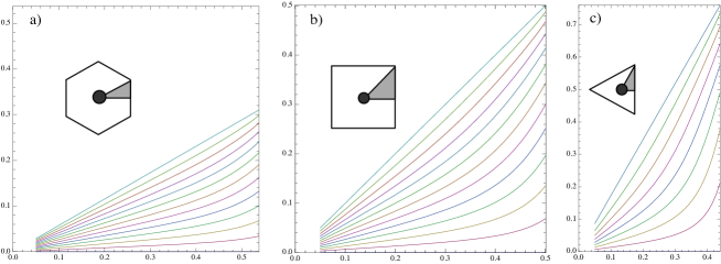
Figure 1: The minimal action paths for the hexagonal (a), square (b), and triangular (c) lattices of cylinders. The gray-shaded regions indicate the computational domain in each cell. Black circles indicate the minority domains.

Under the assumption of Alexander-de Gennes brush for the corona, the integral in (4) is dominated by the minimizers of $H_{A}$ with $\mathbf{r}_{0}\in\Gamma$ fixed and $\mathbf{r}_{N}$ restricted to $\partial\Omega$:

$$F_{\mathrm{corona}}\simeq\nu\int_{\Gamma}\min_{\{\mathbf{r}_{1},\ldots,\mathbf{r}_{N-1}\}}H_{A}\,dA(\mathbf{r}_{0}).$$ (6)

Now, introducing

$$S=\frac{Nb^{2}}{3k_{B}T}\,H_{A},\qquad U=-\frac{N^{2}b^{2}}{3k_{B}T}\,\varphi_{A},$$ (7)

and then passing to continuous chains: $\mathbf{r}_{n}\simeq\mathbf{r}(n/N)$, where $\mathbf{r}:[0,1]\to\Omega_{A}$ are continuous paths, we can write the corona energy as

$$F_{\mathrm{corona}}\simeq\frac{3k_{B}T\nu}{2Nb^{2}}\int_{\Gamma}\int_{0}^{1}\left|\frac{d\mathbf{r}}{dt}\right|^{2}dt\,dA,$$ (8)

where each path $\mathbf{r}(t)$ minimizes

$$S=\int_{0}^{1}\biggl{\{}\frac{1}{2}\left|\frac{d\mathbf{r}}{dt}\right|^{2}-U(\mathbf{r})\biggr{\}}dt$$ (9)

with fixed endpoints.

Note that to be in the mechanical equilibrium the chains must come out normally from the interface $\Gamma$. Then, from the constant monomer density requirement near $\Gamma$ one can get the initial conditions for the minimizers $\mathbf{r}(t)$, given a potential $U(\mathbf{r})$ enforcing the constraint:

$$\mathbf{r}(0)=\mathbf{r}_{0},\qquad\frac{d\mathbf{r}(0)}{dt}=Nv\nu\,\mathbf{n}(\mathbf{r}_{0}),$$ (10)

where $\mathbf{n}$ is the outward (from $\Omega_{B}$) normal to $\Gamma$ at $\mathbf{r}_{0}\in\Gamma$.

We now point out a mechanical analogy, according to which $\mathbf{r}(t)$ can be interpreted as the trajectory of a point particle with unit mass in $\mathbb{R}^{3}$ moving under the action of potential energy $U$. The function $S$ plays the role of the action Landau and Lifshits (1976). Therefore, the equation of motion for $\mathbf{r}(t)$ becomes simply

$$\frac{d^{2}\mathbf{r}}{dt^{2}}=-\nabla U(\mathbf{r}).$$ (11)

Note that the initial condition in (10) then uniquely determines the point at which the trajectory $\mathbf{r}(t)$ hits $\partial\Omega$. We can also easily write down the corresponding Hamilton-Jacobi equation Landau and Lifshits (1976):

$$\frac{d\mathbf{r}}{dt}=\nabla S(\mathbf{r}),\qquad\frac{1}{2}|\nabla S|^{2}+U=U_{0},$$ (12)

where $U_{0}$ is a constant which a posteriori turns out to be independent of the initial point $\mathbf{r}_{0}$ of the trajectory that passes through $\mathbf{r}$.

Note that we still need to determine the self-consistent field, now given by $U$, enforcing the constant monomer density constraint, which in terms of $\mathbf{r}(t)$ becomes

$$\nu N\int_{\Gamma}\int_{0}^{1}\delta(\mathbf{r}-\mathbf{r}(t))dt\,dA=v^{-1},$$ (13)

where $\delta(\mathbf{r})$ is the three-dimensional delta-function, and we assumed that the family of trajectories $\mathbf{r}(t)$ foliates $\Omega_{A}$. On the other hand, observe that it is, in fact, sufficient to find only the action $S$ appearing in (12). The Hamiltonian structure of equation of motion (11) imposes certain restrictions on the possible trajectories $\mathbf{r}(t)$, in particular, it forces the dynamics of $\mathbf{r}$ to be a gradient flow. In fact, it is easy to see that this gradient flow also has to be divergence-free. Indeed, consider a tube formed by trajectories originating on some closed curve in $\Gamma$ enclosing an area $A$, and write down the total number $M$ of A-monomers contained in the cylinder between $t=t_{0}$ and $t=t_{0}+\tau$ cross-sections of that tube. One easily gets $M=\nu NA\tau$, which is clearly independent of $t_{0}$. Hence, differentiating this quantity with respect to $t_{0}$, we see that the total flow in/out of the cylinder along the trajectories must equal zero. In view of arbitrariness of $t_{0},\tau$ and $A$, we must have $\nabla\cdot(d\mathbf{r}/dt)=0$ in $\Omega_{A}$.

The arguments above immediately imply that the action $S$ must be a harmonic function:

$$\Delta S=0~{}\mathrm{in}~{}\Omega_{A},\qquad\mathbf{n}\cdot\nabla S=Nv\nu~{}\mathrm{on}~{}\Gamma,$$ (14)

where $\Delta$ is the Laplacian, and we also used (10). On the other hand, the boundary data on $\partial\Omega$ must be chosen in an unusual way: every trajectory starting on $\Gamma$ at $t=0$ and flowing up the gradient of $S$ must reach $\partial\Omega$ at $t=1$. This condition can also be reformulated as:

$$\int\frac{|d\mathbf{r}|}{|\nabla S(\mathbf{r})|}=1~{}~{}\mathrm{on~{}every~{}field~{}line~{}of~{}}S.$$ (15)

It is also easy to see from (13) that

$$Nv\nu\int_{\Gamma}\int_{0}^{1}\left|\frac{d\mathbf{r}}{dt}\right|^{2}dt\,dA=\int_{\Omega_{A}}|\nabla S|^{2}\,d\mathbf{r}.$$ (16)

With this, the expression for the corona energy becomes

$$F_{\mathrm{corona}}\simeq\frac{3k_{B}T}{2vN^{2}b^{2}}\,D[S],\quad D[S]=\int_{\Omega_{A}}|\nabla S|^{2}\,d\mathbf{r}.$$ (17)

Let us note that existence and uniqueness of solutions to the proposed problem is not guaranteed a priori for any given $\Omega$ and $\Gamma$. In view of (17), one should, in fact, be interested in minimizers of $D[S]$ which also satisfy the condition in (15). Notice that the location of $\Gamma$ relative to $\Omega$ is also part of the minimization problem. A radial solution (presumably, the unique minimizer) trivially exists when $\Omega_{B}$ and $\Omega$ are concentric balls. One would then expect from perturbative considerations that this solution should persist when $\partial\Omega$ is slightly distorted away from a sphere.

In view of the assumption $f\ll 1$, the solution of (14) coincides to the leading order with that of

$$\Delta S=|\Omega|\delta(\mathbf{r}).$$ (18)

Indeed, if $\Omega_{B}$ is a ball of radius $R$ centered at the origin, then $4\pi R^{2}\nu Nv=|\Omega|$ to the leading order in $f$, where $|\Omega|$ denotes the volume of $\Omega$ (same argument applies in two dimensions). From this, one can see that since $S$ should behave as the free space Green’s function of the Laplacian near the origin, $D[S]$ will diverge as $R\to 0$. The leading order singular term will only depend on $|\Omega|$ and not the shape of $\Omega$ and is precisely what was calculated by Semenov for the corona energy Semenov (1985). On the other hand, for small but finite values of $R$ the solution will also contain an excess energy associated with the geometry of $\Omega$.

We applied our variational procedure to compute the excess energy in the case of two-dimensional hexagonal, square, and triangular lattices of straight cylinders $\Omega_{B}$ of radius $R$ and unit height. We note first that the exact solution of the problem in a coaxial cylinder of the same volume $|\Omega|$ gives straightforwardly

$$D_{0}=\frac{|\Omega|^{2}}{4\pi}\ln f^{-1}.$$ (19)

To compute the excess energy $D-D_{0}$ for Wigner-Seitz cells corresponding to the considered lattices, we implemented a finite element-based minimization algorithm to find minimizers of $D$ satisfying (15) Muratov et al. . The minimizing trajectories in cells whose area is normalized to unity are presented in Fig. 1. From dimensional arguments, we find that for $f\ll 1$ we have

$$D-D_{0}\simeq C_{\Omega}|\Omega|^{2},$$ (20)

where the dimensionless constant $C_{\Omega}$ depends on the geometry of the cell only. Numerically, we found $C_{\mathrm{hex}}\simeq 0.00922$, $C_{\mathrm{sq}}\simeq 0.0453$, and $C_{\mathrm{triang}}\simeq 0.179$ for the hexagonal, square, and triangular lattices, respectively. Note that for fixed values of $R$ and $f$ both the interfacial energy $F_{\mathrm{interface}}$, the core energy $F_{\mathrm{core}}$, and the leading-order corona energy $F_{\mathrm{corona}}$ obtained from (17) with $D$ replaced by $D_{0}$ are the same. Therefore, to compare the energies of different geometric arrangements of the B-domains, one needs to compare the excess energies. From our calculation above we can immediately conclude that among the considered types of lattices of cylinders with the same radius $R$ and volume fraction $f$ the hexagonal lattice is the most energetically favorable in the limit $f\to 0$, an intuitively expected result which is put on a rigorous footing by our computations. Let us point out that our approach should also be applicable to spherical phases to help identify the minimizer among different types of three-dimensional lattices. We note that the answer to this question in the strong segregation limit lies beyond the scope of Semenov’s theory Semenov (1985) and its extensions Semenov (1993); Likhtman and Semenov (1994). Let us also point out that the method of Refs. Likhtman and Semenov (1994); Olmsted and Milner (1998) cannot be applied here, since it ignores the effect of the exclusion zone.

Let us note that our calculation is akin to the one performed by Fredrickson Fredrickson (1993), who estimated the excess energy due to geometric factors for a hexagonal Wigner-Seitz cell in the strong segregation limit. Fredrickson used linear elasticity and the Alexander-de Gennes assumption to study the extra contribution to the elastic energy of the corona due to chain distortions. His result, however, differs from ours quantitatively. In particular, we find the excess energy obtained by us is greater than the one obtained by Fredrickson by a factor of 1.5. We attribute this discrepancy to strong chain distortions, which invalidate the linear elasticity approximation. Thus, at small $f$ the excess energy due to geometry of the Wigner-Seitz cell may have a larger contribution than previously expected.

To conclude, we have developed a variational characterization of the leading geometric corrections to the Semenov’s strong segregation theory in the case of strong composition asymmetries. Our theory thus should be able to account for the effect of the confinement geometry on microstructures consisting of small droplets of the minority species and, in particular, help identify the equilibrium lattice configurations of these droplets, as was explicitly demonstrated in the case of cylindrical phases. Perhaps more importantly, our theory provides a new way to study questions of metastability and instability of nonequilibrium copolymer microstructures under external perturbations Ohta and Kawasaki (1986); Muratov (1997, 2002); Matsen (2006).

We wish to thank G. Fredrickson for valuable comments. The work of C. G.-C. was supported by NSF DMS-0505738 grant. C.B.M., M.N., and G.O. gratefully acknowledge support by GNAMPA.

References

- Bates and Fredrickson (1999) F. S. Bates and G. H. Fredrickson, Physics Today 52, 32 (1999).
- Goodman (1982) I. Goodman, ed., Developments in block copolymers (Applied Science Publishers, New York, 1982).
- Aggarwal (1970) S. L. Aggarwal, ed., Block polymers (Plenum Press, New York, 1970).
- Bates and Fredrickson (1990) F. S. Bates and G. H. Fredrickson, Annu. Rev. Phys. Chem. 41, 525 (1990).
- Helfand (1975) E. Helfand, Macromolecules 8, 552 (1975).
- Helfand and Wasserman (1976) E. Helfand and Z. R. Wasserman, Macromolecules 9, 879 (1976).
- Helfand and Wasserman (1978) E. Helfand and Z. R. Wasserman, Macromolecules 11, 960 (1978).
- Helfand and Wasserman (1980) E. Helfand and Z. R. Wasserman, Macromolecules 13, 994 (1980).
- Leibler (1980) L. Leibler, Macromolecules 13, 1602 (1980).
- Semenov (1985) A. N. Semenov, Sov. Phys. JETP 61, 733 (1985).
- Ohta and Kawasaki (1986) T. Ohta and K. Kawasaki, Macromolecules 19, 2621 (1986).
- Likhtman and Semenov (1994) A. E. Likhtman and A. N. Semenov, Macromolecules 27, 3103 (1994).
- Olmsted and Milner (1998) P. D. Olmsted and S. T. Milner, Macromolecules 31, 4011 (1998).
- Matsen and Schick (1994) M. W. Matsen and M. Schick, Phys. Rev. Lett. 72, 2660 (1994).
- Matsen and Whitmore (1996) M. W. Matsen and M. D. Whitmore, J. Chem. Phys. 105, 9698 (1996).
- Groot and Madden (1998) R. D. Groot and T. J. Madden, J. Chem. Phys. 108, 8713 (1998).
- Murat et al. (1999) M. Murat, G. S. Grest, and K. Kremer, Macromolecules 32, 595 (1999).
- Matsen (2001) M. W. Matsen, J. Chem. Phys. 114, 10528 (2001).
- Matsen (2002) M. W. Matsen, J. Phys.: Condens. Matter 14, R21 (2002).
- Schultz et al. (2002) A. J. Schultz, C. K. Hall, and J. Genzer, J. Chem. Phys. 117, 10329 (2002).
- Cochran et al. (2006) E. W. Cochran, C. J. Garcia-Cervera, and G. H. Fredrickson, Macromolecules 39, 2449 (2006), ibid. 39, 4264 (2006).
- Bosse et al. (2006) A. Bosse, S. Sides, K.Katsov, C. García-Cervera, and G. Fredrickson, J. Polym. Sci. Part B: Polym. Phys. 44, 2495 (2006).
- Lambooy et al. (1994) P. Lambooy, T. P. Russell, G. J. Kellogg, A. M. Mayes, P. D. Gallagher, and S. K. Satija, Phys. Rev. Lett. 72, 2899 (1994).
- Knoll et al. (2002) A. Knoll, A. Horvat, K. S. Lyakhova, G. Krausch, G. J. A. Sevink, A. V. Zvelindovsky, and R. Magerle, Phys. Rev. Lett. 89, 035501 (2002).
- Xiang et al. (2004) H. Xiang, K. Shin, T. Kim, S. Moon, T. McCarthy, and T. Russell, Macromolecules 37, 5660 (2004).
- Li et al. (2006) W. Li, R. A. Wickham, and R. A. Garbary, Macromolecules 39, 806 (2006).
- Chen et al. (2007) P. Chen, H. Liang, and A.-C. Shi, Macromolecules 40, 7329 (2007).
- Chantawansri et al. (2007) T. L. Chantawansri, A. W. Bosse, A. Hexemer, H. D. Ceniceros, C. J. García-Cervera, E. J. Kramer, and G. H. Fredrickson, Phys. Rev. E 75, 031802 (2007).
- Yu et al. (2007) B. Yu, P. Sun, T. Chen, Q. Jin, D. Ding, B. Li, and A.-C. Shi, J. Chem. Phys. 126, 204903 (2007).
- Ball et al. (1991) R. C. Ball, J. F. Marko, S. T. Milner, and T. A. Witten, Macromolecules 24, 693 (1991).
- Milner (1991) S. T. Milner, Science 251, 905 (1991).
- Semenov (1993) A. N. Semenov, Macromolecules 26, 2273 (1993).
- Belyi (2004) V. A. Belyi, J. Chem. Phys. 121, 6547 (2004).
- Alexander (1977) S. Alexander, J. de Physique 38, 977 (1977).
- de Gennes (1976) P. G. de Gennes, J. de Physique 37, 1445 (1976).
- Fredrickson (1993) G. H. Fredrickson, Macromolecules 26, 4351 (1993).
- Sijbesma et al. (1997) R. P. Sijbesma, F. H. Beijer, L. Brunsveld, B. J. B. Folmer, J. J. K. K. Hirschberg, R. F. M. Lange, J. K. L. Lowe, and E. W. Meijer, Science 278, 1601 (1997).
- Ruokolainen et al. (1998) J. Ruokolainen, R. Mäkinen, M. Torkkeli, T. Mäkelä, R. Serimaa, G. ten Brinke, and O. Ikkala, Science 280, 557 (1998).
- Landau and Lifshits (1976) L. D. Landau and E. M. Lifshits, Course of Theoretical Physics, vol. 1 (Pergamon Press, London, 1976).
- (40) C. B. Muratov, M. Novaga, G. Orlandi, and C. J. García-Cervera, in preparation.
- Muratov (1997) C. B. Muratov, Phys. Rev. Lett. 78, 3149 (1997).
- Muratov (2002) C. B. Muratov, Phys. Rev. E 66, 066108 (2002).
- Matsen (2006) M. W. Matsen, J. Chem. Phys. 124, 074906 (2006).