Analyzing the Effects of Neutron Polarizabilities in Elastic Compton Scattering off ³He

Abstract

Motivated by the fact that a polarized ³He  nucleus behaves as an ‘effective’ neutron target, we examine manifestations of neutron electromagnetic polarizabilities in elastic Compton scattering from the Helium-3 nucleus. We calculate both unpolarized and double-polarization observables using chiral perturbation theory to next-to-leading order (${\mathcal{O}}(e^{2}Q)$) at energies, $\omega\,\,\raisebox{-3.44444pt}{$\stackrel{{\scriptstyle\textstyle<}}{{\sim}}$ }m_{\pi}$, where $m_{\pi}$ is the pion mass. Our results show that the unpolarized differential cross section can be used to measure neutron electric and magnetic polarizabilities, while two double-polarization observables are sensitive to different linear combinations of the four neutron spin polarizabilities.

I Introduction

The response of an object – that has sub-structure – to a quasi-static electromagnetic (EM) field is characterized in terms of quantities called polarizabilities. For example, when an object, having charged constituents, is placed in an electrostatic field the centers of positive and negative charge separate resulting in an induced electric dipole moment, $\vec{p}=\alpha\vec{E}$, where $\vec{E}$ is the external electrostatic field. The strength of this response, $\alpha$, is defined as the “electric polarizability”. Similarly, we can imagine a magnetic dipole moment $\vec{\mu}=\beta\vec{H}$ being induced in the presence of an external magnetic field, $\vec{H}$, and this magnetic response is quantified in terms of the magnetic polarizability, $\beta$. If an object has intrinsic spin, then in the presence of an EM field the orientation of the spin may be altered. This is the spin-dipole response; in fact, spin responses are quantified in terms of four spin polarizabilities. Here, in this work we shall focus on the electric, magnetic and the spin polarizabilities of the neutron. Investigating the neutron polarizabilities would contribute immensely to our understanding of the neutron structure and also proton-neutron as isospin-doublet. We investigate neutron polarizabilities by calculating elastic Compton scattering off ³He  because there are no free neutron targets and ³He  behaves as an ‘effective’ neutron (as we shall see later).

For the following discussion we consider both the proton and the neutron, which we commonly call nucleon. Using the concept of an effective theory, the most important contributions for the interaction of a nucleon with an EM field can be identified. The interaction Hamiltonian can then be formulated in terms of the EM fields and nucleon EM moments. The symmetries of the EM interaction ensure that only those terms need to be considered that obey the following rules barry :

1. Only terms quadratic in $\vec{A}$ (the EM vector potential) are allowed.

2. The Hamiltonian is gauge invariant,

3. a rotational scalar, and,

4. P (parity), T (time-reversal) even.

Defining $\omega$ as the photon energy, the leading-order response in $\omega$ for a nucleon in an EM field is given by–

$$H^{(0)}_{\mathrm{eff}}=\frac{(\vec{p}-e\vec{A})^{2}}{2M}+e\phi,$$ (1)

where $\vec{A}$ and $\phi$ are the EM vector and scalar potentials. At the next order the following terms appear in the Hamiltonian (see e.g. barry ; Ba98 ):

$$H^{(2)}_{\mathrm{eff}}=-\frac{1}{2}\,4\pi\left[{\alpha}_{E1}\,\vec{E}^{2}+{\beta}_{M1}\,\vec{B}^{2}\right].$$ (2)

Here, ${\alpha}_{E1}$ and ${\beta}_{M1}$ are the electric and magnetic dipole polarizabilities and are the most prominent of the nucleon polarizabilities. This Hamiltonian (Eq. (2)), however, includes only terms of second order in $\omega$ and can be extended, as long as the aforementioned conditions are respected. Apart from $\alpha_{E1}$ and $\beta_{M1}$ there exist other polarizabilities, such as the spin-dependent polarizabilities. Therefore, we can modify and rewrite Eq. (2), extended to the spin dipole polarizabilities barry ; Ba98 :

$$H^{(3)}_{\mathrm{eff}} = -2\pi\,\left[\alpha_{E1}\,\vec{E}^{2}+\beta_{M1}\,\vec{B}^{2}+\gamma_{E1E1}\,\vec{\sigma}\cdot\vec{E}\times\dot{\vec{E}}+\gamma_{M1M1}\,\vec{\sigma}\cdot\vec{B}\times\dot{\vec{B}}\right.$$ (3)

$$-\left.2\,\gamma_{M1E2}\,\sigma_{i}\,E_{ij}\,B_{j}+2\,\gamma_{E1M2}\,\sigma_{i}\,B_{ij}\,E_{j}\right],$$

with $\vec{\sigma}$ denoting the intrinsic nucleon spin. The various subscripts in $\alpha$, $\beta$ and $\gamma$ denote different multipoles of the nucleon’s response to the external EM field and

$$E_{ij} = \frac{1}{2}(\nabla_{i}E_{j}+\nabla_{j}E_{i})$$ (4)

$$B_{ij} = \frac{1}{2}(\nabla_{i}H_{j}+\nabla_{j}H_{i}).$$ (5)

In this work, we use $\gamma_{1}$, $\gamma_{2}$, $\gamma_{3}$ and $\gamma_{4}$ ragusa to represent the four spin polarizabilities and these are related to the $\gamma$’s in Eq. (3) as –

$$\gamma_{E1E1} = -\gamma_{1}-\gamma_{3},$$

$$\gamma_{M1M1} = \gamma_{4},$$

$$\gamma_{M1E2} = \gamma_{2}+\gamma_{4},$$

$$\gamma_{E1M2} = \gamma_{3}.$$ (6)

An electromagnetic probe by nature, Compton scattering captures information about the response of the charge and current distributions inside a nucleon, and hence the polarizabilities, to a quasi-static electromagnetic field. To lowest order in photon energy (${\mathcal{O}}(\omega^{0})$), the spin-averaged amplitude for Compton scattering on the nucleon is given by the Thomson term

$${\rm Amp}=-\frac{{\mathcal{Z}}^{2}e^{2}}{M}\hat{\epsilon}\cdot\hat{\epsilon}^{\prime},$$ (7)

where ${\mathcal{Z}}e,M$ represent the nucleon charge and mass respectively and $\hat{\epsilon},\hat{\epsilon}^{\prime}$ specify the polarization vectors of the initial and final photons respectively. At the next order in photon energy, contributions arise from electric and magnetic polarizabilities—$\bar{\alpha}_{E}$ and $\bar{\beta}_{M}$—which measure the response of the nucleon to the application of quasi-static electric and magnetic fields. The spin-averaged amplitude is expressed in the laboratory frame as:

$${\rm Amp}={\hat{\epsilon}}\cdot{\hat{\epsilon}\,^{\prime}}\left(-\frac{{\mathcal{Z}}^{2}e^{2}}{M}+\omega\omega^{\prime}\;4\pi\bar{\alpha}_{E}\right)+{\hat{\epsilon}}\times\hat{k}\cdot{\hat{\epsilon}\,^{\prime}}\times{\hat{k}\,^{\prime}}\;\omega\omega^{\prime}4\pi\bar{\beta}_{M}+\;{\mathcal{O}}(\omega^{4})\;.$$ (8)

Here, $k_{\mu}=(\omega,\vec{k})$, ${k^{\prime}}_{\mu}=(\omega^{\prime},\vec{k}^{\prime})$ specify the four-momenta of the initial and final photons respectively and $\hat{k}$ and ${\hat{k}\,^{\prime}}$ are unit vectors associated with the photon momenta. When we square the amplitude (8), the associated differential scattering cross section on the proton is given by

$${d\sigma\over d\Omega} = \left({e^{2}\over 4\pi M}\right)^{2}\left({\omega^{\prime}\over\omega}\right)^{2}\left[{1\over 2}(1+\cos^{2}\theta)\right.$$

$$- \left.{4\pi M\omega\omega^{\prime}\over e^{2}}\left({1\over 2}(\bar{\alpha}_{E}+\bar{\beta}_{M})(1+\cos\theta)^{2}+{1\over 2}(\bar{\alpha}_{E}-\bar{\beta}_{M})(1-\cos\theta)^{2}\right)+\ldots\right].$$

(9)

From Eq. (9) it is evident that the differential cross-section is sensitive to $(\bar{\alpha}_{E}+\bar{\beta}_{M})$ at forward angles and to $(\bar{\alpha}_{E}-\bar{\beta}_{M})$ at backward angles.

It is essential to mention here that for the purpose of this work, $\bar{\alpha}_{E}$ and $\bar{\beta}_{M}$ are the so-called Compton polarizabilities and measure the “true deformation” effect on the nucleon. In other words, Compton polarizabilities measure the distortion effects of charge and current distributions inside a nucleon subjected to an EM field. In the non-relativistic limit, these reduce to the static electromagnetic polarizabilities described in Eq. (2). For example, the static electric polarizability, $\alpha_{E1}=\bar{\alpha}_{E}+{\kappa^{2}\over M}$ Ba97 , where $\kappa$ is the anomalous magnetic moment of the nucleon and $M$ is its mass. From here on we shall drop the subscripts $E$ and $M$ as well as the bars over $\alpha$ and $\beta$ from the Compton polarizabilities. Therefore all polarizabilities discussed from now on are the Compton polarizabilities. At the next order in $\omega$ beyond that considered in Eq. (8), one can access the spin polarizabilities ($\gamma$’s) of the nucleon.

The last fifteen years or so has been witness to a concerted effort on the part of both theorists and experimentalists to comprehend the structure of nucleons as manifested in Compton scattering. Through various experiments on the proton, its electric and magnetic polarizabilities have been effectively pinned down. There has been an avalanche of experimental data on unpolarized Compton scattering on the proton at photon energies below 200 MeV Fe91 ; Ze92 ; Ha93 ; Ma95 ; Ol01 . The current Particle Data Group (PDG) values for the proton are:

$$\alpha_{p} = (12.0\pm 0.6)\times 10^{-4}\,{\rm fm}^{3},$$

$$\beta_{p} = (1.9\pm 0.5)\times 10^{-4}\,{\rm fm}^{3}.$$ (10)

Most of the extractions of the proton electromagnetic polarizabilities were performed via a dispersion relation approach by a multipole analysis of the photoabsorption amplitudes Ar96 ; Lv97 . Calculations have also been done up to $\mathcal{O}(e^{2}Q^{2})$ in $\chi$PT  McG01 ; Be02 ; Be04 and these calculations give a very impressive description of the data for $\omega$, $\sqrt{|t|}<$200 MeV.

Note that it is necessary to measure only one of $\alpha$ and $\beta$. In practice, one can then use the dispersion sum rule (Baldin sum rule) derived from the optical theorem bkmrev

$$\alpha+\beta=\frac{1}{2\pi^{2}}\int_{\omega_{th}}^{\infty}\frac{\sigma_{p}^{tot}(\omega)}{\omega^{2}}\,\mathrm{d}\omega,$$ (11)

that relates the sum of the polarizabilities to the total photoabsorption cross-section in order to extract the other. In Eq. (11), $\sigma_{p}^{tot}(\omega)$ is the total photoabsorption cross-section and $\omega_{th}$ is the pion-production threshold. For the proton Ol01 ,

$$\alpha_{p}+\beta_{p}=(13.8\pm 0.4)\times 10^{-4}\,{\rm fm}^{3}.$$ (12)

There are several evaluations of the dispersion relation in Eq. (11) for the neutron nbaldin ; Ba98 ; Lv00 . However, there is discrepancy between the numbers extracted. A recent extraction of the sum rule by Levchuk and L’vov Lv00 using relevant neutron photo-production multipoles gives

$$\alpha_{n}+\beta_{n}=(15.2\pm 0.5)\times 10^{-4}\,{\rm fm}^{3}.$$ (13)

Because of the discrepancy in the extraction of the neutron sum rule, as far as the neutron polarizabilities go, we still strive to extract precise numbers for the polarizabilities. Since neutrons are very short-lived, we lack free neutron targets and this poses a serious handicap in the study of neutron structure. The drawback caused by not having free neutron targets encouraged the community to look at other avenues to extract information about the neutron.

There were attempts to measure neutron polarizabilities via scattering neutrons on lead to access the Coulomb field of the target and examining the cross-section as a function of energy. Currently there is much controversy over what this technique gives for $\alpha_{n}$. Two experiments using this same technique obtained different results for $\alpha_{n}$ (Refs. Sc91 ; Ko95 ).

$$\alpha_{n} = (12.6\pm 1.5\pm 2.0)\times 10^{-4}\,{\rm fm}^{3};$$ (14)

$$\alpha_{n} = (0.6\pm 5.0)\times 10^{-4}\,{\rm fm}^{3}.$$ (15)

Enik et al En97 revisited Ref. Sc91 (Eq. (14)) and recommended a value of $\alpha_{n}$ between $7\times 10^{-4}$ fm³ and $19\times 10^{-4}$ fm³.

In addition, quasi-free Compton scattering from the deuteron was measured at SAL Ko00a for incident photon energies of $E_{\gamma}=(236-260)$ MeV and one-sigma constraints on the polarizabilities were reported to be:

$$\alpha_{n} = (7.6-14.0)\times 10^{-4}\,{\rm fm}^{3},$$

$$\beta_{n} = (1.2-7.6)\times 10^{-4}\,{\rm fm}^{3}.$$ (16)

Another quasi-free experiment was performed at Mainz Ko03 and the difference in the polarizabilities was obtained:

$$\alpha_{n}-\beta_{n}=(9.8\pm 3.6{\rm(stat)}\pm 2.2{\rm(model)}{}^{+2.1}_{-1.1}{\rm(sys)})\times 10^{-4}\,{\rm fm}^{3}.$$ (17)

Until now, however, there have been only limited efforts to measure nucleon spin polarizabilities. The only ones that have been extracted from the experimental data are the forward and backward spin polarizabilities. The backward spin polarizability is defined as:

$$\gamma_{\pi}=\gamma_{1}+\gamma_{2}+2\gamma_{4}.$$ (18)

The neutron backward spin polarizability was determined to be

$$\gamma_{\pi n}=(58.6\pm 4.0)\times 10^{-4}\,{\rm fm}^{4},$$ (19)

from quasi-free Compton scattering on the deuteron Ko03 . This experiment used the Mainz 48 cm $\varnothing\times$ 64 cm NaI detector and the Göttingen recoil detector SENECA in coincidence. For comparison, an experiment Ca02 using the same detector set-up extracted a proton backward polarizability value ranging from (-36.5 to -39.1)$\times 10^{-4}$ fm⁴. These values are consistent with earlier Mainz measurements Ol01 ; Ga01 ; Wo01 .

The theoretical prediction for $\gamma_{\pi p}$ from $\chi$PT is $-36.7\times 10^{-4}$ fm⁴ He98 ; Pa03 and these calculations were done up to the next-to-leading order with the $\Delta$-isobar as an explicit degree of freedom. The prediction $\chi$PT for $\gamma_{\pi n}$ is $57.4\times 10^{-4}$ fm⁴ Pa03 . Both predictions are in agreement with the experimental numbers to within their quoted uncertainties.

The forward spin polarizability, $\gamma_{0}$, is related to energy-weighted integrals of the difference in the helicity-dependent photoreaction cross-sections ($\sigma_{1/2}-\sigma_{3/2}$). Using the optical theorem one can derive the following sum rule for the forward spin polarizability bkmrev ; ggt :

$$\gamma_{0}=\gamma_{1}-(\gamma_{2}+2\gamma_{4})=\frac{1}{4\pi^{2}}\int_{\omega_{th}}^{\infty}\frac{\sigma_{1/2}-\sigma_{3/2}}{\omega^{3}}\,\mathrm{d}\omega,$$ (20)

where $\omega_{th}$ is the pion-production threshold. The following results on $\gamma_{0}$ were estimated using the VPI-FA93 multipole analysis Sa94 to calculate the integral on the RHS of Eq. (20):

$$\gamma_{0p} \simeq -1.34\times 10^{-4}\,{\rm fm}^{4},$$ (21)

$$\gamma_{0n} \simeq -0.38\times 10^{-4}\,{\rm fm}^{4}.$$ (22)

The $\chi$PT prediction for $\gamma_{0p}$ is $-2.1\times 10^{-4}$ fm⁴ Pa03 and for $\gamma_{0n}$ is consistent with 0 Pa03 .

Let us now summarize the “state of the nucleon polarizabilities”. The quantities $\alpha_{p}$ and $\beta_{p}$ are well known, $\alpha_{n}$ and $\beta_{n}$ are also known. However, looking at the numbers in Eqs. (13)–(17), it is evident that the extractions of $\alpha_{n}$ and $\beta_{n}$ have large error bars. Strikingly, there is no consensus on the numbers for $\gamma_{1p}\ldots\gamma_{4p}$ or on $\gamma_{1n}\ldots\gamma_{4n}$. Of these, $\gamma_{1p}\ldots\gamma_{4p}$ are not known due to a lack of experimental data. But it is clear that the extraction of $\alpha_{n}$, $\beta_{n}$ and $\gamma_{1n}\ldots\gamma_{4n}$ require efforts from both the theoretical and the experimental community.

As there are no free neutron targets, the theoretical community has directed focus on elastic Compton scattering from light nuclei to access the neutron polarizabilities. The main advantage of such a reaction process compared to the more complex n-Pb scattering is that the theoretical analysis of the few-body reactions is much better controlled. The lightest nucleus is the deuteron and elastic $\gamma d$ scattering has been studied with the intent of extracting information about the neutron polarizabilities from unpolarized and polarization observables. It should be noted, however, that processes with $A>1$ pose a different kind of challenge because they require an understanding of the inter-nucleon interaction. Deuteron structure is governed by the NN interaction and hence, when analyzing $\gamma$d data, one has to include the effects of photons coupling to mesons being exchanged between nucleons (‘two-body currents’) over and above the single-nucleon $\gamma$N amplitude. There exist calculations for $\gamma$d scattering in the framework of conventional potential models We83 ; Wi95a ; Lv95 ; Lv98 ; Lv00 ; Ka99 . All of these calculations use a realistic NN interaction and usually give a good description of the data. However, the predictions of these calculations depend somewhat on the NN model chosen. $\chi$PT on the other hand allows a model independent framework to systematically build the theory for $\gamma$d scattering. The amplitude for coherent Compton scattering on the deuteron has been calculated to $\mathcal{O}(e^{2}Q^{2})$ by Beane et. al. Be02 ; Be04 . At this order there are four new parameters in the theory (two of which can be fit to the $\gamma p$ data) and since the deuteron is an isoscalar, the nucleon isoscalar polarizabilities were extracted from the above experimental data by fitting the other two parameters. The isoscalar polarizabilities are linear combinations of the proton and neutron polarizabilities, $\alpha_{N}\equiv{(\alpha_{p}+\alpha_{n})\over 2}$ and $\beta_{N}\equiv{(\beta_{p}+\beta_{n})\over 2}$. Beane $et\,al.$ obtained–

$$\alpha_{N} = (8.9\pm 1.5)^{+4.7}_{-0.9}\times 10^{-4}\,{\rm fm}^{3},$$

$$\beta_{N} = (2.2\pm 1.5)^{+1.2}_{-0.9}\times 10^{-4}\,{\rm fm}^{3}.$$ (23)

Subsequently, next-to-leading order calculations for deuteron Compton scattering have been performed that include the $\Delta$ as an explicit degree of freedom and also incorporate the low-energy NN rescattering contributions in the intermediate state Hi05a ; Hi05b ; Hi05 . Thus, sophisticated calculations on $\gamma$d scattering already exist and with more experimental data soon to come from MAXLab in Sweden there is hope that $\alpha_{n}$ and $\beta_{n}$ can be extracted with good precision from that experiment.

Recent experimental advances (for example technology to polarize targets) have made it possible to venture into the area of polarization observables. Hildebrandt $et\,al.$ Hi04b ; Hi05 have also studied polarization observables for Compton scattering on the nucleon (both proton and neutron) with a focus on the spin polarizabilities. Their calculation involves free nucleons and may be beneficial for understanding processes that involve quasi-free kinematics like $\gamma d\rightarrow\gamma np$. Choudhury and Phillips Ch05 ; mythesis focused on $\vec{\gamma}d\rightarrow\gamma d$ and $\vec{\gamma}\vec{d}\rightarrow\gamma d$ to analyze the effects of the electric, magnetic and the spin polarizabilities of the neutron. They reported that one of the double-polarization observables was sensitive to a linear combination of the neutron spin polarizabilities and the deuteron Compton scattering observables alone were not enough to extract the neutron polarizabilities. Calculations for polarization observables for deuteron Compton scattering with explicit $\Delta$-isobar and low-energy resummation have also been completed and the results are forthcoming Sh08 .

These studies We83 ; Wi95a ; Lv95 ; Lv98 ; Lv00 ; Ka99 ; Be99 ; Be02 ; Be04 ; Hi05a ; Hi05b ; Hi04b ; Hi05 ; Ch05 ; mythesis ; Sh08 make it evident that not all of the neutron polarizabilities can be extracted from deuteron Compton scattering. This means that several different observables or combinations of observables from different reactions are necessary to effectively pin down the neutron polarizabilities. To this end, physicists should focus on other alternatives, for instance, quasi-free kinematics in deuteron Compton scattering, or other nuclear targets to extract information about the neutron. Such parallel calculations to study the effect of the same neutron polarizabilities combined with experiments can build confidence in the extraction of the polarizabilities. In principle, one should extract the same numbers, no matter what the process or the target is. Thus, these parallel studies would reassure us about our understanding of “nuclear” effects.

One alternative target is the polarized ³He  nucleus. This nucleus has the nice property that the two proton spins are anti-aligned for the most dominant part of the ³He  wavefunction, the principal ‘$s$-state’. Since approximately 90% of the wavefunction is given by this state, the spin of ³He  nucleus is mostly carried by the unpaired neutron alone. Fig. 1 shows the configurations for the principal ‘$s$-state’ and for one other possible contributions to the ³He  wavefunction he3pol ; No03 . This paper reports our calculations for Compton scattering on a ³He  nucleus.

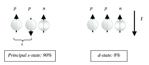
Figure 1: The polarized ³He  nucleus. 90% of the time the nucleus is in the principal s-state configuration.

Note that, for $\gamma$³He  scattering we now have to understand the interplay of the three nucleons over and above the two-nucleon effects.

In this work, we calculate elastic Compton scattering on $\,{}^{3}$He to $\mathcal{O}(e^{2}Q)$ and focus on specific observables so as to construct road-maps to extract the neutron polarizabilities, $\alpha_{n}$, $\beta_{n}$ and $\gamma_{1n}\ldots\gamma_{4n}$. It should be mentioned here that these are the first  ³He Compton scattering calculations in any framework. These calculations include the processes $\gamma^{3}$He$\rightarrow\gamma^{3}$He and $\vec{\gamma}\vec{{}^{3}He}\rightarrow\gamma^{3}$He and are necessarily exploratory. They are expected to provide benchmark results for elastic Compton scattering on $\,{}^{3}$He. As such, our results will serve to attract further explorations of these observables at $\mathcal{O}(e^{2}Q^{2})$ and beyond. The main conclusions of this work have already been reported in Ref. long ; mythesis . This paper is intended to be a comprehensive discussion on the calculations that lead to these conclusions.

This paper is organized in the following manner. Sec. II lays out the structure of our calculation. In Sec. III we describe the various observable that we focus on and then Sec. V we report our results. In order to make this work comprehensive, a discussion on inherent sources of uncertainties that may affect the final result is provided in Sec. VII. Finally, in Sec. VIII, the calculation is summarized and also future directions for calculations of $\gamma$³He  scattering are pointed out.

II Anatomy of the Calculation

The irreducible amplitudes for the elastic scattering of real photons from the NNN system are first ordered and calculated in HB$\chi$PT . Then these amplitudes are sandwiched between the nuclear wavefunctions to finally obtain the scattering amplitudes (see Fig. 2). This amplitude can be written as–

$${\mathcal{M}}=\langle\Psi_{f}|{\hat{O}}|\Psi_{i}\rangle$$ (24)

Here, $|\Psi_{i}\rangle$ or $|\Psi_{f}\rangle$ are the ³He  wavefunctions that are anti-symmetrized in order to take into account that the nucleons are identical fermions. We will employ ³He  wavefunctions obtained from Faddeev calculations in momentum space. We first calculate a specific Faddeev component $|\psi\rangle_{3}$ for ³He  which is related to the fully anti-symmetrized wavefunction $|\Psi\rangle$ No97 by

$$|\Psi\rangle=(1+P)|\psi\rangle_{3}$$ (25)

where $P=P_{31}P_{12}+P_{32}P_{12}$ is the sum of the cyclic and anti-cyclic permutation operators and the numbered subscripts denote the nucleon number.

Figure 2: The anatomy of the calculation. The irreducible amplitude is computed in HB$\chi$PT and sandwiched between external ³He  wavefunctions to give the matrix element for Compton scattering on ³He .

In our case, since we are calculating only up to $\mathcal{O}(e^{2}Q)$ in HB$\chi$PT , the operator ${\hat{O}}$ consists of a one-body part

$${\hat{O}}^{1B}={\hat{O}}^{1B}(1)+{\hat{O}}^{1B}(2)+{\hat{O}}^{1B}(3),$$ (26)

and a two-body part

$${\hat{O}}^{2B}={\hat{O}}^{2B}(1,2)+{\hat{O}}^{2B}(2,3)+{\hat{O}}^{2B}(3,1).$$ (27)

The mechanisms that contribute to the two different pieces are shown in Figs. 3, 4 and 5. The structure of the $\gamma$N and the $\gamma$NN amplitudes follows Refs. bkmrev ; Be99 and they are shown in Apps. A and B. In the notation used in Eq. (26), ${\hat{O}}^{1B}(a),a=1\ldots 3$ represents the one-body current where the external photon interacts with nucleon ‘$a$’ and in Eq. (27), ${\hat{O}}^{2B}(a,b)$ represents a two-body current where the external photon interacts with the nucleon pair ‘$(a,b)$’. In short, the different terms in Eqs. (26) and (27) represent different permutations of the three nucleons inside ³He . Note that, we do not have any three-body currents because they appear only at ${\mathcal{O}}(e^{2}Q^{3})$ in the $\chi$PT power-counting.

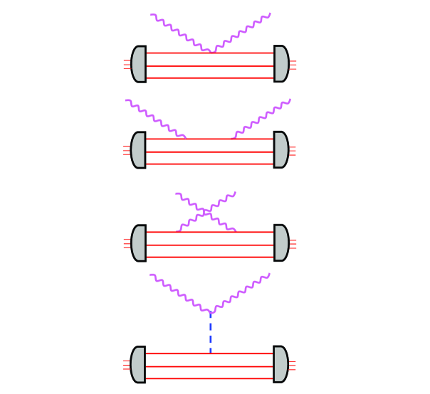
Figure 3: Tree level diagrams for the one-body amplitude.

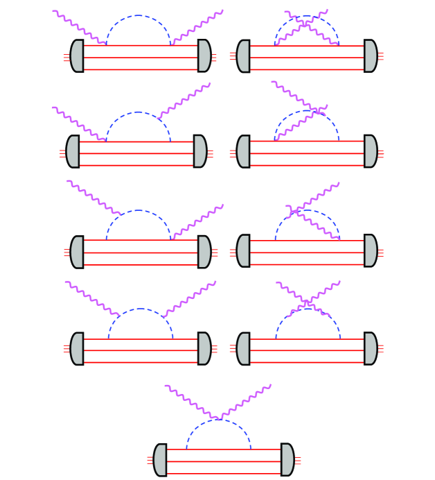
Figure 4: Contribution to the one-body amplitude at $\mathcal{O}(e^{2}Q)$. These diagrams contain one pion loop.

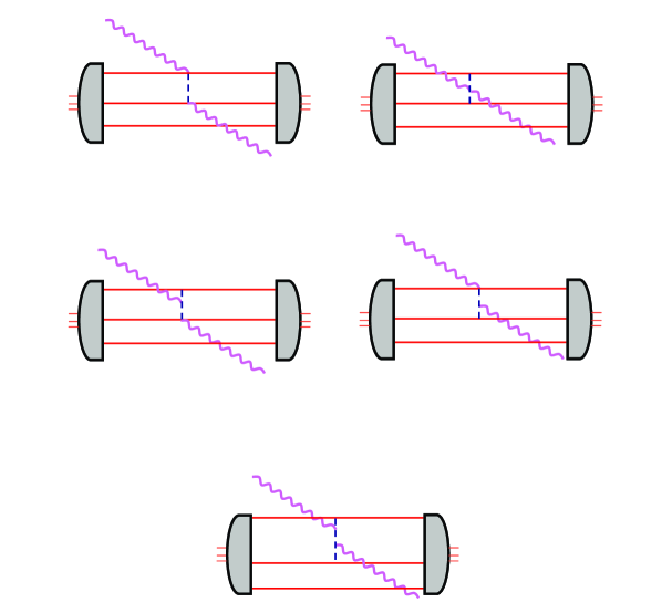
Figure 5: Contributing two-body diagrams at $\mathcal{O}(e^{2}Q)$. Permutations are not shown.

If we now take into account the identity of the three nucleons, we can rewrite Eq. (24) as–

$${\mathcal{M}}=3\langle\Psi_{f}|{\hat{O}}^{1B}(1)+{\hat{O}}^{2B}(1,2)|\Psi_{i}\rangle$$ (28)

For our calculations we draw upon the work of Kotlyar et al Ko00 . They developed an approach for calculating matrix elements of meson-exchange current operators between three-nucleon basis states. They applied this approach in studying ³He  photo- and electro-disintegration. The three-nucleon basis states were expressed in a $jj$-coupling scheme (final configuration) and a three-nucleon bound state (initial configuration). These matrix elements were then expressed in terms of multiple integrals in momentum space. Since they studied photo- and electro-disintegration, they had only one external momentum transfer vector $\vec{q}$ that they could choose to align in a preferred direction in order to simplify the calculations. Here in contrast, since we have an incoming and outgoing photon with different three-momenta, we do not have the same liberty and hence we needed to extend their prescription. Also, we choose to calculate the one-body currents too in the two-nucleon spin-isospin basis and hence it is more convenient to express Eq. (28) as–

$${\mathcal{M}}=3\langle\Psi_{f}|\frac{1}{2}\big{(}{\hat{O}}^{1B}(1)+{\hat{O}}^{1B}(2)\big{)}+{\hat{O}}^{2B}(1,2)|\Psi_{i}\rangle=3\langle\Psi_{f}|{\hat{O}}(1,2)|\Psi_{i}\rangle.$$ (29)

The advantage of this formulation is that the structure of the calculation is similar for both the one-body and the two-body parts. The next step is then to actually calculate the matrix elements. To do this, we project the state-vectors and the operators on to the basis–

$$|p_{12}p_{3}\,\alpha\rangle=|p_{12}p_{3}\rangle|(l_{12}s_{12})j_{12}(l_{3}{1\over 2})j_{3}(j_{3}j_{12})JM_{J}\rangle|(t_{12}{1\over 2})TM_{T}\rangle_{3}=|p_{12}p_{3}\rangle|\alpha_{J}\rangle|\alpha_{T}\rangle_{3}.$$ (30)

Here, $p_{12}$ and $p_{3}$ denote the magnitude of the Jacobi momenta of the pair “(1,2)” and the spectator nucleon “3” and this choice ensures that the set of basis states are complete and orthonormalized. The subscript ‘3’ represents the choice of the Jacobi momenta (Fig. 6) defined as–

$$\vec{p}_{12} = {1\over 2}(\vec{k}_{2}-\vec{k}_{1})$$

$$\vec{p}_{3} = {1\over 3}(2\vec{k}_{3}-\vec{k}_{2}-\vec{k}_{1}).$$ (31)

$i.e.$ nucleon ‘3’ serves as the spectator.

Figure 6: Jacobi momenta for the three-nucleon system.

The total angular momentum of the nucleus $J$ is a result of coupling between $j_{12}$ and $j_{3}$, the total angular momenta of the ‘(1,2)’ subsystem and the spectator nucleon ‘3’ respectively. The orbital angular momentum $l_{12}$ and the spin $s_{12}$ of the two-body subsystem ‘(1,2)’ combine to give $j_{12}$ and similarly, $l_{3}$ and $s_{3}={1\over 2}$ combine to give $j_{3}$. $t_{12}$ is the isospin of the two-nucleon subsystem and it combines with the isospin of the spectator nucleon to give the total isospin $T$ and $M_{T}$ is simply the projection of $T$. Since we are concerned with the ³He  nucleus–

$$|TM_{T}\rangle = |{1\over 2}{1\over 2}\rangle$$

$$|JM_{J}\rangle = |{1\over 2}M_{J}\rangle.$$ (32)

The basis states as defined above are not completely anti-symmetrized. The antisymmetry is carried by the complete wavefunction. However, for the two-body subsystem quantum numbers the antisymmetry within the subsystem leads to the additional constraint that $l_{12}+s_{12}+t_{12}=2n+1,(n=0,1,2,\ldots)$.

Before delving into the matrix element calculations, let us first consider the kinematics of Compton scattering from a ³He  nucleus with momenta assigned in this way.

II.1 Kinematics

Since we are interested in two-body currents at the most, the kinematics of our problem becomes a little simplified. In our calculations we shall be working in the $\gamma\,^{3}$He c.m. frame.

Figure 7: The kinematics of the calculation in $\gamma$³He  c.m. frame. The vectors $\vec{k}$ ($-\vec{k}$) and $\vec{k}^{\prime}$ ($-\vec{k}^{\prime}$) are the three-momenta of the incoming and outgoing photon (³He) in the $\gamma$³He  c.m. frame.

As we can see in Fig. 7, nucleon “3” serves as a mere spectator to the $\gamma$NN $\rightarrow\gamma$NN scattering process and this means that in our calculations we can treat the “(1,2)” and “3” momentum spaces separately. Moreover, since the third nucleon does not partake in the interaction, we have a three-momentum conserving delta-function from–

$$\vec{p}_{3}\,^{\prime}-{\vec{k}^{\prime}\over 3} = \vec{p}_{3}-{\vec{k}\over 3}$$

$$\Rightarrow\vec{p}_{3}\,^{\prime} = \vec{p}_{3}+{(\vec{k}^{\prime}-\vec{k})\over 3}$$ (33)

$$= \vec{p}_{3}+{\vec{q}\over 3},$$

where, $\vec{q}=(\vec{k}^{\prime}-\vec{k})$. Hence, in principle, any integral in $\vec{p}_{3}\,^{\prime}$ space can be eliminated by using this simplification. However, as is evident from Fig. 7, there are still three unknown three-momenta and hence we have to perform a nine-dimensional integral to calculate the matrix elements. We shall see later that the matrix-elements pertaining to the one-body currents are further reduced to six-dimensional integrals because of an additional three-momentum conserving delta-function.

Figure 8: The co-ordinate system.

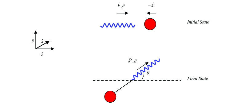
Figure 9: Compton scattering - before and after picture.

Before we go further into the discussion of the calculation, let us first mention that in the subsequent descriptions the following convention for the co-ordinate system is used (see Fig. 8). The beam direction is defined as the $z$ axis. The $x-z$ plane is the scattering plane with the $y$ axis being normal to it. Fig. 9 shows the before and after picture for Compton scattering from a target. The wiggly line depicts a photon, the red circle depicts the target. As mentioned earlier, the scattering takes place in the $x-z$ plane with $\theta$ defining the angle of scattering in the center of mass (c.m.) frame. For linearly polarized photons, the polarization vectors in the initial state can be along the $x$ or the $y$ axis, $i.e.$, ${\hat{\epsilon}}=\hat{x}$ or $\hat{y}$. For circularly polarized photons in the initial state, the beam helicity, $\lambda$, can be $\pm 1$. The photons are right circularly polarized (RCP) if the beam helicity, $\lambda=+1$ (${\hat{\epsilon}}_{+}=-\frac{\hat{x}+i\hat{y}}{\sqrt{2}}$) or left circularly polarized (LCP) if the beam helicity, $\lambda=-1$ (${\hat{\epsilon}}_{-}=\frac{\hat{x}-i\hat{y}}{\sqrt{2}}$).

II.2 The Matrix Element

Focusing back on our matrix element calculation, we now introduce complete sets of momentum states to obtain–

$${\mathcal{M}}(M_{J}^{\prime},M_{J}) = 3\langle\Psi_{f}{({1\over 2};M_{J}^{\prime})}|{\hat{O}}(1,2)|\Psi_{i}{({1\over 2};M_{J})}\rangle$$ (34)

$$= 3\int d^{3}p_{12}\,^{\prime}\int d^{3}p_{3}\,^{\prime}\int d^{3}p_{12}\int d^{3}p_{3}\sum\limits_{\alpha,\alpha^{\prime},m_{12},m_{12}^{\prime}}$$

$$\langle\Psi_{f}{({1\over 2};M_{J}^{\prime})}|\vec{p}_{12}\,^{\prime}\vec{p}_{3}\,^{\prime}\alpha^{\prime}\rangle\langle\vec{p}_{12}\,^{\prime}\vec{p}_{3}\,^{\prime}\alpha^{\prime}|{\hat{O}}(1,2)|\vec{p}_{12}\vec{p}_{3}\alpha\rangle\langle\vec{p}_{12}\vec{p}_{3}\alpha|\Psi_{i}{({1\over 2};M_{J})}\rangle$$

$$= \int d^{3}p_{12}\,^{\prime}\int d^{3}p_{3}\,^{\prime}\int d^{3}p_{12}\int d^{3}p_{3}$$

$$\sum\limits_{\alpha,\alpha^{\prime},m_{12},m_{12}^{\prime}}\varphi(p_{12}\,^{\prime},p_{3}\,^{\prime},\alpha^{\prime})\varphi(p_{12},p_{3},\alpha)$$

$${\mathcal{Y}}_{l_{12}^{\prime},s_{12}^{\prime},j_{12}^{\prime},m_{12}^{\prime}}^{*}(\hat{p}_{12}\,^{\prime}){\mathcal{Y}}_{l_{3}^{\prime},{1\over 2},j_{3}^{\prime},M_{J}^{\prime}-m_{12}^{\prime}}^{*}(\hat{p}_{3}\,^{\prime})\delta(\vec{p}_{3}\,^{\prime}-(\vec{p}_{3}+{\vec{q}\over 3}))$$

$$\langle\vec{p}_{12}\,^{\prime}\vec{p}_{3}\,^{\prime};\alpha_{T}^{\prime}|{\hat{O}}(1,2)|\vec{p}_{12}\vec{p}_{3};\alpha_{T}\rangle{\mathcal{Y}}_{l_{12},s_{12},j_{12},m_{12}}(\hat{p}_{12}){\mathcal{Y}}_{l_{3},{1\over 2},j_{3},M_{J}-m_{12}}(\hat{p}_{3}).$$

where $|\Psi_{i}({1\over 2};M_{J})\rangle$ and $\langle\Psi_{f}({1\over 2};M_{J}^{\prime})|$ denote that the ³He nucleus is in a specific isospin and total spin projected state. In Eq. (34), we define

$${\mathcal{Y}}_{l,s,j,m}(\hat{p})=\sum\limits_{m_{s}}(l,m-m_{s},s,m_{s}|l,s,j,m)Y_{l,m-m_{s}}(\hat{p})|sm_{s}\rangle$$ (35)

and

$$\varphi(p_{12},p_{3},\alpha)=(j_{12},m_{12},j_{3},M_{J}-m_{12}|j_{12},j_{3},J,M_{J})$$

$$(t_{12},mt_{12},{1\over 2},mt_{3}|t_{12},{1\over 2},{1\over 2},{1\over 2})\langle p_{12}p_{3}\alpha|\Psi\rangle.$$ (36)

where the ³He  wavefunction $\langle p_{12}p_{3}\alpha|\Psi\rangle$ is independent of $M_{J}$.

For a consistent calculation of the matrix element, the nuclear interaction used to generate the ³He  wavefunction should be based on the same chiral effective field theory approach that we used for the derivation of the operators. Strictly speaking, the available nuclear interactions have been derived in slightly different frameworks. Therefore, in order to get an idea of the dependence of our results on the choice of the wavefunction, we have employed several nuclear interactions to obtain the ³He  wavefunctions. These are the chiral $NLO$ interactions of Refs. Ep99 ; Ep00 , the chiral Idaho $N^{3}LO$ interaction En03 and the high precision model interaction Wi95 . In order to correct for the underbinding of the ³He  system when only NN interactions are used, we augment these interactions also by NNN interactions No06 ; Pu95 as specified later. Based on this range of interactions, the binding energy of ³He  is between 6.89–7.83 MeV (the experimental one is 7.72 MeV). It turns out that a rather small number of partial waves is sufficient to sufficient to achieve convergence for the Compton scattering matrix elements. We found that the one-body (two-body) matrix elements are converged to within 0.1% (0.2%) using partial waves with $j_{12}\leq$2 ($j_{12}\leq$1).

In the sum in Eq. (34), we can use the fact that the isospin projection of the third particle remains unchanged, as does the total isospin projection, to introduce the kronecker-delta $\delta_{mt_{12}^{\prime},mt_{12}}$. Eq. (34) is a 12-dimensional integral and it can be reduced to a 10-dimensional one by simply implementing the delta-functions over the angular parts of $\vec{p_{3}\,^{\prime}}$. Since we are separating the angular and magnitude part of the three-momenta, from here on we shall drop the ‘vector’ sign in the momenta; for example $|\vec{p}_{3}\,^{\prime}|\equiv p_{3}\,^{\prime}$. This leads to–

$${\mathcal{M}}(M_{J}^{\prime},M_{J}) = 3\sum\limits_{j_{12}^{\prime},j_{12},m_{12}^{\prime},m_{12},s_{12}^{\prime},s_{12},l_{12}^{\prime},l_{12},j_{3}^{\prime},j_{3},l_{3}^{\prime},l_{3},mt_{12}}$$ (37)

$$\int p_{12}\,^{\prime 2}dp_{12}\,^{\prime}\int p_{12}^{2}dp_{12}\int dp_{3}^{\prime}\int p_{3}^{2}dp_{3}$$

$$\varphi(p_{12}\,^{\prime},p_{3}\,^{\prime},\alpha^{\prime})\varphi(p_{12},p_{3},\alpha)$$

$$\int d{\hat{p}_{12}\,^{\prime}}\int d{\hat{p}_{12}}{\mathcal{Y}}_{l_{12}^{\prime},s_{12}^{\prime},j_{12}^{\prime},m_{12}^{\prime}}^{*}(\hat{p}_{12}\,^{\prime})\langle\vec{p}_{12}\,^{\prime};t_{12}^{\prime}mt_{12}|{\hat{O}}(1,2)|\vec{p}_{12};t_{12}mt_{12}\rangle$$

$${\mathcal{Y}}_{l_{12},s_{12},j_{12},m_{12}}(\hat{p}_{12})\int d{\hat{p}_{3}}{\mathcal{Y}}_{l_{3}^{\prime},{1\over 2},j_{3}^{\prime},M_{J}^{\prime}-m_{12}^{\prime}}^{*}\left(\widehat{p_{3}+{q\over 3}}\right)$$

$$\delta\left(p_{3}\,^{\prime}-|\vec{p_{3}}+\vec{{q\over 3}}|\right){\mathcal{Y}}_{l_{3},{1\over 2},j_{3},M_{J}-m_{12}}(\hat{p}_{3})$$

$$= 3\sum\limits_{j_{12}^{\prime},j_{12},m_{12}^{\prime},m_{12},s_{12}^{\prime},s_{12},l_{12}^{\prime},l_{12},j_{3}^{\prime},j_{3},l_{3}^{\prime},l_{3},mt_{12}}$$

$$\int p_{12}\,^{\prime 2}dp_{12}\,^{\prime}\int p_{12}^{2}dp_{12}\int p_{3}^{2}dp_{3}\varphi(p_{12},p_{3},\alpha)$$

$${\mathcal{I}}_{2}(p_{12},p_{12}\,^{\prime};l_{12},l_{12}^{\prime},s_{12},s_{12}^{\prime},j_{12},j_{12}^{\prime},m_{12},m_{12}^{\prime},mt_{12})$$

$$\int dp_{3}\,^{\prime}\varphi(p_{12}\,^{\prime},p_{3}\,^{\prime},\alpha^{\prime}){\mathcal{I}}_{3}(p_{3},p_{3}^{\prime};l_{3},l_{3}^{\prime},j_{3},j_{3}^{\prime},m_{12},m_{12}^{\prime},M_{J},M_{J}^{\prime}).$$

The integral

$${\mathcal{I}}_{2}(p_{12},p_{12}\,^{\prime};l_{12},l_{12}^{\prime},s_{12},s_{12}^{\prime},j_{12},j_{12}^{\prime},m_{12},m_{12}^{\prime},mt_{12})=$$

$$\int d{\hat{p}_{12}\,^{\prime}}\int d{\hat{p}_{12}}\,{\mathcal{Y}}_{l_{12}^{\prime},s_{12}^{\prime},j_{12}^{\prime},m_{12}^{\prime}}^{*}(\hat{p}_{12}\,^{\prime})$$

$$\langle\vec{p}_{12}\,^{\prime};t_{12}^{\prime}mt_{12}|{\hat{O}}(1,2)|\vec{p}_{12};t_{12}mt_{12}\rangle{\mathcal{Y}}_{l_{12},s_{12},j_{12},m_{12}}(\hat{p}_{12})$$ (38)

is a four-dimensional integral and is computed numerically. By using the delta-function we can reduce the dimensionality of

$${\mathcal{I}}_{3}(p_{3},p_{3}^{\prime};l_{3},l_{3}^{\prime},j_{3},j_{3}^{\prime},m_{12},m_{12}^{\prime},M_{J},M_{J}^{\prime})=$$

$$\int d{\hat{p}_{3}}{\mathcal{Y}}_{l_{3}^{\prime},{1\over 2},j_{3}^{\prime},M_{J}^{\prime}-m_{12}^{\prime}}^{*}\left(\widehat{p_{3}+{q\over 3}}\right)\delta\left(p_{3}\,^{\prime}-|\vec{p_{3}}+\vec{{q\over 3}}|\right){\mathcal{Y}}_{l_{3},{1\over 2},j_{3},M_{J}-m_{12}}(\hat{p}_{3})$$ (39)

which is two-dimensional, thereby making the final integral a nine-dimensional one. We shall first talk about how ${\mathcal{I}}_{3}(p_{3},p_{3}^{\prime};l_{3},l_{3}^{\prime},j_{3},j_{3}^{\prime},m_{12},m_{12}^{\prime},M_{J},M_{J}^{\prime})$ is reduced and then focus on ${\mathcal{I}}_{2}(p_{12},p_{12}\,^{\prime};l_{12},l_{12}^{\prime},s_{12},s_{12}^{\prime},j_{12},j_{12}^{\prime},m_{12},m_{12}^{\prime},mt_{12})$. However, even at that point our job is far from being done because the operators also have to be evaluated in this same basis. We shall discuss this procedure right after we finish discussing how the integrals were calculated.

II.2.1 Reduction of Integral ${\mathcal{I}}_{3}$

As noted in Eq. (37), ${\mathcal{I}}_{3}$ is a two-dimensional integral involving the angular integration of the momentum ${\vec{p_{3}}}$. However, we can translate the delta-function in ${\vec{|p_{3}\,^{\prime}}}|$ to one that involves the azimuthal angle of ${\vec{p_{3}}}$ using the following steps.

$$\delta\left(p_{3}\,^{\prime}-|\vec{p_{3}}+\vec{q\over 3}|\right) = 2p_{3}\,^{\prime}\delta\left(p_{3}\,^{\prime 2}-|\vec{p_{3}}+\vec{q\over 3}|^{2}\right)$$ (40)

$$= 2p_{3}\,^{\prime}\delta\left(p_{3}\,^{\prime 2}-p_{3}^{2}-{q^{2}\over 9}-\frac{2p_{3}q}{3}(\widehat{p_{3}\cdot q})\right).$$

Since, we work in the co-ordinate system defined in Sec. II.1, ${\hat{k}}=(0,0,1)$ and ${\hat{k}^{\prime}}=(\sin\theta,0,\cos\theta)$ and this means that ${\hat{q}}$ is in the $x-z$ plane or $\phi_{q}=0$. Then defining ${\hat{p_{3}}}=(\sin\theta_{3}\cos\phi_{3},\sin\theta_{3}\sin\phi_{3},\cos\theta_{3})$ we can rewrite Eq. (40) as–

$$\delta\left(p_{3}\,^{\prime}-|\vec{p_{3}}+\vec{q\over 3}|\right) = \frac{3p_{3}\,^{\prime}}{p_{3}q}\frac{1}{\sin\theta_{3}\sin\theta_{q}}\delta\left(\cos\phi_{3}-\frac{z_{3}-\cos\theta_{3}\cos\theta_{q}}{\sin\theta_{3}\sin\theta_{q}}\right)$$ (41)

$$= \frac{3p_{3}\,^{\prime}}{p_{3}q}\frac{1}{\sin\theta_{3}\sin\theta_{q}}\frac{1}{|\sin\tilde{\phi_{3}}|}\left[\delta(\phi_{3}-\tilde{\phi_{3}})+\delta(\phi_{3}+\tilde{\phi_{3}})\right],$$

where,

$$z_{3} = \frac{p_{3}\,^{\prime 2}-p_{3}^{2}-{q^{2}\over 9}}{\frac{2p_{3}q}{3}}$$

$$\cos\tilde{\phi_{3}} = \frac{z_{3}-\cos\theta_{3}\cos\theta_{q}}{\sin\theta_{3}\sin\theta_{q}}.$$ (42)

Using Eq. (41) we can now eliminate the $\phi_{3}$ integral in ${\mathcal{I}}_{3}$. The delta-function $\delta\left(p_{3}\,^{\prime}-|\vec{p_{3}}+\vec{q\over 3}|\right)$ further sets the bounds of integration for both the $p_{3}\,^{\prime}$ and the $\theta_{3}$ integrals. Implementing the above steps, we can now express the last line of Eq. (37) as–

$$\int dp_{3}\,^{\prime}\varphi(p_{12}\,^{\prime},p_{3}\,^{\prime},\alpha^{\prime}){\mathcal{I}}_{3}(p_{3},p_{3}^{\prime};l_{3},l_{3}^{\prime},j_{3},j_{3}^{\prime},m_{12},m_{12}^{\prime},M_{J},M_{J}^{\prime})=$$ (43)

$$\int\limits_{|{p_{3}}-{q\over 3}|}^{{p_{3}}+{q\over 3}}dp_{3}\,^{\prime}\varphi(p_{12}\,^{\prime},p_{3}\,^{\prime},\alpha^{\prime})\frac{3p_{3}\,^{\prime}}{p_{3}q\sin\theta_{q}}$$

$$\int\limits_{|\theta_{q}-\arccos z_{3}|}^{\theta_{q}+\arccos z_{3}}\sin\theta_{3}d\theta_{3}\frac{1}{|\sin\tilde{\phi_{3}}|\sin\theta_{3}}\sum\limits_{ms_{3}^{\prime},ms_{3}}\delta_{ms_{3}^{\prime},ms_{3}}$$

$$(l_{3}^{\prime},M_{J}^{\prime}-m_{12}^{\prime}-ms_{3}^{\prime},{1\over 2},ms_{3}^{\prime}|l_{3}^{\prime},{1\over 2},j_{3}^{\prime},M_{J}^{\prime}-m_{12}^{\prime})$$

$$(l_{3},M_{J}-m_{12}-ms_{3},{1\over 2},ms_{3}|l_{3},{1\over 2},j_{3},M_{J}-m_{12})$$

$$([Y_{l_{3}^{\prime},M_{J}^{\prime}-m_{12}^{\prime}-ms_{3}^{\prime}}^{*}(\widehat{p_{3}+{q\over 3}})Y_{l_{3},M_{J}-m_{12}-ms_{3}}(\hat{p_{3}})]_{\phi_{3}=\tilde{\phi_{3}}}$$

$$+[Y_{l_{3}^{\prime},M_{J}^{\prime}-m_{12}^{\prime}-ms_{3}^{\prime}}^{*}(\widehat{p_{3}+{q\over 3}})Y_{l_{3},M_{J}-m_{12}-ms_{3}}(\hat{p_{3}})]_{\phi_{3}=-\tilde{\phi_{3}}})$$

$$= \int\limits_{|{p_{3}}-{q\over 3}|}^{{p_{3}}+{q\over 3}}dp_{3}\,^{\prime}\varphi(p_{12}\,^{\prime},p_{3}\,^{\prime},\alpha^{\prime})\tilde{{\mathcal{I}}_{3}}(p_{3},p_{3}^{\prime};l_{3},l_{3}^{\prime},j_{3},j_{3}^{\prime},m_{12},m_{12}^{\prime},M_{J},M_{J}^{\prime}).$$

with $\tilde{{\mathcal{I}}_{3}}(p_{3},p_{3}^{\prime};l_{3},l_{3}^{\prime},j_{3},j_{3}^{\prime},m_{12},m_{12}^{\prime},M_{J},M_{J}^{\prime})$ as a one-dimensional integral over $\theta_{3}$. The kronecker-delta $\delta_{ms_{3}^{\prime},ms_{3}}$ comes from the fact that our operator does not act on the spin of the third nucleon. Thus, the final expression for the matrix element looks like–

$${\mathcal{M}}(M_{J}^{\prime},M_{J}) = 3\sum\limits_{j_{12}^{\prime},j_{12},m_{12}^{\prime},m_{12},s_{12}^{\prime},s_{12},l_{12}^{\prime},l_{12},j_{3}^{\prime},j_{3},l_{3}^{\prime},l_{3},mt_{12}}$$ (44)

$$\int p_{12}\,^{\prime 2}dp_{12}\,^{\prime}\int p_{12}^{2}dp_{12}\int p_{3}^{2}dp_{3}\varphi(p_{12},p_{3},\alpha)$$

$${\mathcal{I}}_{2}(p_{12},p_{12}\,^{\prime};l_{12},l_{12}^{\prime},s_{12},s_{12}^{\prime},j_{12},j_{12}^{\prime},m_{12},m_{12}^{\prime},mt_{12})$$

$$\int\limits_{|{p_{3}}-{q\over 3}|}^{{p_{3}}+{q\over 3}}dp_{3}\,^{\prime}\varphi(p_{12}\,^{\prime},p_{3}\,^{\prime},\alpha^{\prime})$$

$$\tilde{{\mathcal{I}}_{3}}(p_{3},p_{3}^{\prime};l_{3},l_{3}^{\prime},j_{3},j_{3}^{\prime},m_{12},m_{12}^{\prime},M_{J},M_{J}^{\prime}).$$

II.2.2 Further Reduction of One-Body Matrix Elements

At this point, we would like to recall that the operator has a one-body and a two-body part and the kinematics make it further evident that the one-body calculations should be simpler and involve fewer integrals. The one-body matrix element is–

$${\mathcal{M}}=3\langle\Psi_{f}|\frac{1}{2}\big{(}{\hat{O}}^{1B}(1)+{\hat{O}}^{1B}(2)\big{)}|\Psi_{i}\rangle={3\over 2}(\langle\Psi_{f}|{\hat{O}}^{1B}(1,2)|\Psi_{i}\rangle)$$ (45)

where ${\hat{O}}^{1B}(1,2)$ is the one-body operator in the two-nucleon spin-isospin space. This means that only one of the three nucleons is involved in the scattering process and we are gifted with yet another three-momentum conserving delta-function. For the purpose of this discussion, considering nucleon ‘1’ (see Fig. 7) as the ‘struck’ nucleon, we can use–

$$-\vec{p}_{12}\,^{\prime}-{\vec{p}_{3}\,^{\prime}\over 2}-{\vec{k}^{\prime}\over 3} = -\vec{p}_{12}-{\vec{p}_{3}\over 2}-{\vec{k}\over 3}$$

$$\Rightarrow\vec{p}_{12}\,^{\prime} = \vec{p}_{12}-{\vec{q}\over 2},$$ (46)

after using Eq. (33). We have to be careful here because in our calculations we use the basis of two-nucleon spin and isospin. However, we use the fact that the spin and isospin sums are performed only over allowed partial waves and hence we can assume that nucleon ‘1’ is the struck nucleon and use Eq. (46) to relate $\vec{p}_{12}\,^{\prime}=\vec{p}_{12}-{\vec{q}\over 2}$. This is very useful because we can now reduce integral ${\mathcal{I}}_{2}$ in the same manner as ${\mathcal{I}}_{3}$. After going through all the steps described in Sec. II.2.1 we arrive at–

$${\mathcal{M}}^{1B}(M_{J}^{\prime},M_{J}) = {3\over 2}\sum\limits_{j_{12}^{\prime},j_{12},m_{12}^{\prime},m_{12},s_{12}^{\prime},s_{12},l_{12}^{\prime},l_{12},j_{3}^{\prime},j_{3},l_{3}^{\prime},l_{3},mt_{12}}$$ (47)

$$\int p_{12}^{2}dp_{12}\int p_{3}^{2}dp_{3}\varphi(p_{12},p_{3},\alpha)$$

$$\int\limits_{|{p_{3}}-{q\over 3}|}^{{p_{3}}+{q\over 3}}dp_{3}\,^{\prime}\int\limits_{|{p_{12}}-{q\over 2}|}^{p_{12}+{q\over 2}}dp_{12}\,^{\prime}\varphi(p_{12}\,^{\prime},p_{3}\,^{\prime},\alpha^{\prime})$$

$$\tilde{{\mathcal{I}}_{2}}(p_{12},p_{12}\,^{\prime};l_{12},l_{12}^{\prime},s_{12},s_{12}^{\prime},j_{12},j_{12}^{\prime},m_{12},m_{12}^{\prime},mt_{12})$$

$$\tilde{{\mathcal{I}}_{3}}(p_{3},p_{3}^{\prime};l_{3},l_{3}^{\prime},j_{3},j_{3}^{\prime},m_{12},m_{12}^{\prime},M_{J},M_{J}^{\prime}).$$

where,

$$\tilde{{\mathcal{I}}_{2}}(p_{12},p_{12}\,^{\prime};l_{12},l_{12}^{\prime},s_{12},s_{12}^{\prime},j_{12},j_{12}^{\prime},m_{12},m_{12}^{\prime},mt_{12})$$ (48)

$$= \frac{2p_{12}\,^{\prime}}{p_{12}q\sin\theta_{q}}\int\limits_{|\theta_{q}-\arccos z_{12}|}^{\theta_{q}+\arccos z_{12}}\sin\theta_{12}d\theta_{12}$$

$$\frac{1}{|\sin\tilde{\phi_{12}}|\sin\theta_{12}}\sum\limits_{ms_{12}^{\prime},ms_{12}}$$

$$(l_{12}^{\prime},m_{12}^{\prime}-ms_{12}^{\prime},s_{12}^{\prime},ms_{12}^{\prime}|l_{12}^{\prime},s_{12}^{\prime},j_{12}^{\prime},m_{12}^{\prime})$$

$$(l_{12},m_{12}-ms_{12},s_{12},ms_{12}|l_{12},s_{12},j_{12},m_{12})$$

$$([Y_{l_{12}^{\prime},m_{12}^{\prime}-ms_{12}^{\prime}}^{*}(\widehat{p_{12}-{q\over 2}})Y_{l_{12},m_{12}-ms_{12}}(\hat{p_{12}})]_{\phi_{12}=\tilde{\phi_{12}}}$$

$$+[Y_{l_{12}^{\prime},m_{12}^{\prime}-ms_{12}^{\prime}}^{*}(\widehat{p_{12}-{q\over 2}})Y_{l_{12},m_{12}-ms_{12}}(\hat{p_{12}})]_{\phi_{12}=-\tilde{\phi_{12}}})$$

$$\langle t_{12}^{\prime}mt_{12}|\langle s_{12}^{\prime}ms_{12}^{\prime}|{\hat{O}}^{1B}(1,2)|s_{12}ms_{12}\rangle|t_{12}mt_{12}\rangle$$

and,

$$z_{12} = \frac{p_{12}^{2}+{q^{2}\over 4}-p_{12}\,^{\prime 2}}{p_{12}q}$$

$$\cos\tilde{\phi_{12}} = \frac{z_{12}-\cos\theta_{12}\cos\theta_{q}}{\sin\theta_{12}\sin\theta_{q}}.$$ (49)

Now that we have the structure of the matrix elements, let us look at the operators. We have to translate the one-body operator (from App. A) and the two-body operators (from App. B) into the two-nucleon spin-isospin space.

II.2.3 One-Body operator in Two-Nucleon Spin-Isospin Space

The one-body operator as described in App. A can not be used directly. So, using Eq. (2) we write–

$${\hat{O}}^{1B}(1,2)=T_{\gamma N}^{(1)}+T_{\gamma N}^{(2)}=\sum\limits_{i=1\ldots 6}(A_{i}^{(1)}t_{i}^{(1)}+A_{i}^{(2)}t_{i}^{(2)})$$ (50)

where $t_{i}$ are the operators involving the photon polarization, momenta and nucleon spin and the superscripts ‘(1)’ and ‘(2)’ refer to specific nucleons. Then defining

$$A_{i}=A_{i}^{(IS)}+A_{i}^{(IV)}\tau_{3}$$ (51)

where, the superscripts $(IS)$ and $(IV)$ refer to isoscalar and isovector pieces of $A_{i}$ respectively, we can rewrite Eq. (50) as–

$${\hat{O}}^{1B}(1,2) = \sum\limits_{i=1\ldots 6}[A_{i}^{(IS)}(t_{i}^{(1)}+t_{i}^{(2)})+A_{i}^{(IV)}(t_{i}^{(1)}\tau_{3}^{(1)}+t_{i}^{(2)}\tau_{3}^{(2)})]$$ (52)

$$= \sum\limits_{i=1\ldots 6}[A_{i}^{(IS)}(t_{i}^{(1)}+t_{i}^{(2)})+{1\over 2}A_{i}^{(IV)}\{(\tau_{3}^{(1)}+\tau_{3}^{(2)})(t_{i}^{(1)}+t_{i}^{(2)})$$

$$+(\tau_{3}^{(1)}-\tau_{3}^{(2)})(t_{i}^{(1)}-t_{i}^{(2)})\}].$$

And we have,

$$\langle t_{12}^{\prime}mt_{12}|(\tau_{3}^{(1)}+\tau_{3}^{(2)})|t_{12}mt_{12}\rangle=2$$ (53)

only for $t_{12}^{\prime}=t_{12}=1$ and $mt_{12}=1$. (We do not consider the case when $mt_{12}=-1$ because it is not possible for a ³He  nucleus.) Also,

$$\langle t_{12}^{\prime}mt_{12}|(\tau_{3}^{(1)}-\tau_{3}^{(2)})|t_{12}mt_{12}\rangle=1$$ (54)

for $\langle 10|\leftarrow|00\rangle$ and $\langle 00|\leftarrow|10\rangle$ only and the rest are zero.

For the spin part of the operator we have either $(t_{i}^{(1)}+t_{i}^{(2)})$ or $(t_{i}^{(1)}-t_{i}^{(2)})$. And we can write–

$$(t_{i}^{(1)}+t_{i}^{(2)})=2(t_{1}+t_{2})+2i\sum\limits_{i=3\ldots 6}\vec{S}\cdot\vec{V}_{i}$$ (55)

where $\vec{S}$ is the total spin operator of the two-nucleon system and $\vec{V}_{i}$ is a vector that contains the photon polarization and momenta. Similarly,

$$(t_{i}^{(1)}-t_{i}^{(2)})=i\sum\limits_{i=3\ldots 6}(\vec{\sigma}^{(1)}-\vec{\sigma}^{(2)})\cdot\vec{V}_{i}$$ (56)

This operator induces the transitions $\langle 00|\leftarrow|1ms_{12}\rangle$ and $\langle 1ms_{12}^{\prime}|\leftarrow|00\rangle$.

II.2.4 The One-Body Matrix Element

At this point, lets summarize how the different pieces combine to give ${\mathcal{M}}^{1B}(M_{J}^{\prime},M_{J})$. Since, $\tilde{{\mathcal{I}}_{3}}(p_{3},p_{3}^{\prime};l_{3},l_{3}^{\prime},j_{3},j_{3}^{\prime},m_{12},m_{12}^{\prime},M_{J},M_{J}^{\prime})$ does not have any pieces of the Compton operator, it is calculated separately. Then using the information from Eqs. (53) and (54) we calculate the isospin matrix elements in two-body isospin space. Now, for each of the non-zero isospin transitions, the spin transition matrix elements are calculated using the information from Eqs. (55) and (56), $i.e.$ by calculating the expectation values of $\vec{S}$ or $(\vec{\sigma}^{(1)}-\vec{\sigma}^{(2)})$ between two-nucleon spin states as dictated by Eq. (52). Now that we have $\langle t_{12}^{\prime}mt_{12}|\langle s_{12}^{\prime}ms_{12}^{\prime}|{\hat{O}}^{1B}(1,2)|s_{12}ms_{12}\rangle|t_{12}mt_{12}\rangle$, we put this in Eq. (48) and numerically calculate $\tilde{{\mathcal{I}}_{2}}(p_{12},p_{12}\,^{\prime};l_{12},l_{12}^{\prime},s_{12},s_{12}^{\prime},j_{12},j_{12}^{\prime},$$m_{12},m_{12}^{\prime},mt_{12})$. Then we plug in the values of $\tilde{{\mathcal{I}}_{3}}(p_{3},p_{3}^{\prime};l_{3},l_{3}^{\prime},j_{3},j_{3}^{\prime},m_{12},m_{12}^{\prime},M_{J},M_{J}^{\prime})$ and $\tilde{{\mathcal{I}}_{2}}(p_{12},p_{12}\,^{\prime};l_{12},l_{12}^{\prime},s_{12},s_{12}^{\prime},j_{12},j_{12}^{\prime},m_{12},m_{12}^{\prime},mt_{12})$ in Eq. (47), evaluate the integrals over $p_{3}\,^{\prime}$, $p_{3}$, $p_{12}\,^{\prime}$ and $p_{12}$ after introducing the wavefunctions projected into the equivalent basis and finally, sum over all angular momentum and isospin quantum numbers to obtain ${\mathcal{M}}^{1B}(M_{J}^{\prime},M_{J})$.

Next, we shall describe the procedure for the two-body operators and put everything back together to obtain the two-body matrix element.

II.2.5 Structure of Two-Body Matrix Elements

The two-body matrix element can be written as–

$${\mathcal{M}}^{2B}(M_{J}^{\prime},M_{J}) = 3\sum\limits_{j_{12}^{\prime},j_{12},m_{12}^{\prime},m_{12},s_{12}^{\prime},s_{12},l_{12}^{\prime},l_{12},j_{3}^{\prime},j_{3},l_{3}^{\prime},l_{3},mt_{12}}$$ (57)

$$\int p_{12}^{2}dp_{12}\int p_{12}\,^{\prime 2}dp_{12}\,^{\prime}\int p_{3}^{2}dp_{3}\varphi(p_{12},p_{3},\alpha)$$

$$\int\limits_{|{p_{3}}-{q\over 3}|}^{{p_{3}}+{q\over 3}}dp_{3}\,^{\prime}\varphi(p_{12}\,^{\prime},p_{3}\,^{\prime},\alpha^{\prime})$$

$${\mathcal{I}}_{2}(p_{12},p_{12}\,^{\prime};l_{12},l_{12}^{\prime},s_{12},s_{12}^{\prime},j_{12},j_{12}^{\prime},m_{12},m_{12}^{\prime},mt_{12})$$

$$\tilde{{\mathcal{I}}_{3}}(p_{3},p_{3}^{\prime};l_{3},l_{3}^{\prime},j_{3},j_{3}^{\prime},m_{12},m_{12}^{\prime},M_{J},M_{J}^{\prime}).$$

where, ${\mathcal{I}}_{2}(p_{12},p_{12}\,^{\prime};l_{12},l_{12}^{\prime},s_{12},s_{12}^{\prime},j_{12},j_{12}^{\prime},m_{12},m_{12}^{\prime},mt_{12})$ in its entire glory is given by–

$${\mathcal{I}}_{2}(p_{12},p_{12}\,^{\prime};l_{12},l_{12}^{\prime},s_{12},s_{12}^{\prime},j_{12},j_{12}^{\prime},m_{12},m_{12}^{\prime},mt_{12})=$$

$$\int d{\hat{p}_{12}\,^{\prime}}\int{\hat{p}_{12}}{\mathcal{Y}}_{l_{12}^{\prime},s_{12}^{\prime},j_{12}^{\prime},m_{12}^{\prime}}^{*}(\hat{p}_{12}\,^{\prime})$$

$$\langle\vec{p}_{12}\,^{\prime};t_{12}^{\prime}mt_{12}|{\hat{O}}(1,2)|\vec{p}_{12};t_{12}mt_{12}\rangle{\mathcal{Y}}_{l_{12},s_{12},j_{12},m_{12}}(\hat{p}_{12})$$

$$=\int d{\hat{p}_{12}\,^{\prime}}\int{\hat{p}_{12}}\sum\limits_{ms_{12},m_{12}^{\prime}}(l_{12}^{\prime},m_{12}^{\prime}-ms_{12}^{\prime},s_{12}^{\prime},ms_{12}^{\prime}|l_{12}^{\prime},s_{12}^{\prime},j_{12}^{\prime},m_{12}^{\prime})$$

$$(l_{12},m_{12}-ms_{12},s_{12},ms_{12}|l_{12},s_{12},j_{12},m_{12})$$

$$Y^{*}_{l_{12}^{\prime},m_{12}^{\prime}-ms_{12}^{\prime}}(\hat{p}_{12}\,^{\prime})Y_{l_{12},m_{12}-ms_{12}}(\hat{p}_{12})$$

$$\langle\vec{p}_{12}\,^{\prime};t_{12}^{\prime}mt_{12}s_{12}^{\prime}ms_{12}^{\prime}|{\hat{O}}^{2B}(1,2)|\vec{p}_{12};t_{12}mt_{12}s_{12}ms_{12}\rangle$$ (58)

Let us then see how $\langle\vec{p}_{12}\,^{\prime};t_{12}^{\prime}mt_{12}^{\prime}s_{12}^{\prime}ms_{12}^{\prime}|{\hat{O}}^{2B}(1,2)|\vec{p}_{12};t_{12}mt_{12}s_{12}ms_{12}\rangle$ is evaluated.

II.2.6 Two-Body Operator in Two-Nucleon Spin-Isospin Space

The two-body operator is given by Eq. (1) and each of the terms in that equation are expressed in the equations following it. Symbolically, we can write each of those diagrams as (for example, for the first diagram in Fig. 5)–

$$T_{\gamma NN}^{(a)} = -\frac{{e^{2}}{g_{A}^{2}}}{2f_{\pi}^{2}}\;({\vec{\tau}}^{\;(1)}\cdot{\vec{\tau}}^{\;(2)}-\tau^{(1)}_{3}\tau^{(2)}_{3})\frac{{{\hat{\epsilon}}\cdot{\vec{\sigma}^{\scriptscriptstyle 1}}}\;{{\hat{\epsilon}\,^{\prime}}\cdot{\vec{\sigma}^{\scriptscriptstyle 2}}}}{2[{\omega^{2}}-{m_{\pi}^{2}}-({\vec{p}}-{{\vec{p}}\,^{\prime}}+{\frac{1}{2}({\vec{k}}+{{\vec{k}}\,^{\prime}})})^{2}]}$$ (59)

$$= \digamma^{(a)}({\vec{\tau}}^{(1)}\cdot{\vec{\tau}}^{(2)}-\tau^{(1)}_{3}\tau^{(2)}_{3}){{\hat{\epsilon}}\cdot{\vec{\sigma}^{\scriptscriptstyle 1}}}\;{{\hat{\epsilon}\,^{\prime}}\cdot{\vec{\sigma}^{\scriptscriptstyle 2}}}$$

In general, the spin-isospin structure of the two-body operator would be–

$$\digamma^{(..)}({\vec{\tau}}^{(1)}\cdot{\vec{\tau}}^{(2)}-\tau^{(1)}_{3}\tau^{(2)}_{3}){{\vec{\sigma}^{\scriptscriptstyle 1}}\cdot\vec{A}}\;{{\vec{\sigma}^{\scriptscriptstyle 2}}\cdot\vec{B}}.$$ (60)

The only transitions in isospin space that are non-zero are $\langle 00|\leftarrow|00\rangle$ and $\langle 10|\leftarrow|10\rangle$ and both of these are–

$$\langle 00|({\vec{\tau}}^{\;(1)}\cdot{\vec{\tau}}^{\;(2)}-\tau^{(1)}_{3}\tau^{(2)}_{3})|00\rangle=-\langle 10|({\vec{\tau}}^{\;(1)}\cdot{\vec{\tau}}^{\;(2)}-\tau^{(1)}_{3}\tau^{(2)}_{3})|10\rangle=-2.$$ (61)

For the spin part of the operator we can write–

$${{\vec{\sigma}^{\scriptscriptstyle 1}}\cdot\vec{A}}\;{{\vec{\sigma}^{\scriptscriptstyle 2}}\cdot\vec{B}}={1\over 2}({\hat{O}}_{s}+{\hat{O}}_{a})$$ (62)

where ${\hat{O}}_{s}$ is the symmetric combination of the LHS of Eq. (62) and ${\hat{O}}_{a}$ is the asymmetric combination under the interchange of nucleons. Then, we can write ${\hat{O}}_{s}$ as–

$${\hat{O}}_{s}=4\vec{S}\cdot\vec{A}\vec{S}\cdot\vec{B}-2\vec{A}\cdot\vec{B}-2i\vec{S}\cdot(\vec{A}\times\vec{B}).$$ (63)

Here, $2\vec{S}={\vec{\sigma}^{\scriptscriptstyle 1}}+{\vec{\sigma}^{\scriptscriptstyle 2}}$ and we have used the identity ${\sigma\cdot\vec{A}}\;{\sigma\cdot\vec{B}}=\vec{A}\cdot\vec{B}+i\vec{\sigma}\cdot(\vec{A}\times\vec{B})$. Since this is a spin-symmetric combination ${\hat{O}}_{s}$ induces the transitions $\langle 00|\leftarrow|00\rangle$ and $\langle 1ms_{12}^{\prime}|\leftarrow|1ms_{12}\rangle$. The different spin transition matrix elements can be written in terms of general vectors $\vec{A}$ and $\vec{B}$ as –

$$\langle 00|{\hat{O}}_{s}|00\rangle = -2\vec{A}\cdot\vec{B}$$

$$\langle 1ms_{12}^{\prime}|{\hat{O}}_{s}|1ms_{12}\rangle = -2\vec{A}\cdot\vec{B}\delta_{ms_{12}^{\prime},ms_{12}}$$ (64)

$$+8\sum\limits_{\mu\alpha\beta}(1,\alpha,1,\mu|1,1,1,ms_{12}^{\prime})(1,\beta,1,ms_{12}|1,1,1,\mu)A_{\alpha}^{\dagger}B_{\beta}^{\dagger}$$

$$+i2\sqrt{2}\sum\limits_{\gamma}(1,\gamma,1,ms_{12}|1,1,1,ms_{12}^{\prime})(\vec{A}\times\vec{B})_{\gamma}^{\dagger}$$

where we have introduced spherical components of vectors $\vec{A}$ and $\vec{B}$. Similarly, we can simplify the asymmetric combination to–

$${\hat{O}}_{a}=2\vec{S}\cdot\vec{A}({\vec{\sigma}^{\scriptscriptstyle 1}}-{\vec{\sigma}^{\scriptscriptstyle 2}})\cdot\vec{B}-i({\vec{\sigma}^{\scriptscriptstyle 1}}-{\vec{\sigma}^{\scriptscriptstyle 2}})\cdot(\vec{A}\times\vec{B}).$$ (65)

This, being a spin-asymmetric combination, it induces transitions between $\langle 00|\leftarrow|1ms_{12}\rangle$ or $\langle 1ms_{12}^{\prime}|\leftarrow|00\rangle$. After going through some spin algebra we obtain–

$$\langle 1ms_{12}^{\prime}|{\hat{O}}_{a}|00\rangle = 2\sqrt{2}\sum\limits_{\alpha\beta}(1,\alpha,1,\beta|1,1,1,ms_{12}^{\prime})A_{\alpha}^{\dagger}B_{\beta}^{\dagger}$$ (66)

$$-i\sum\limits_{\gamma}\delta_{ms_{12}^{\prime},\gamma}(\vec{A}\times\vec{B})_{\gamma}^{\dagger}.$$

We can calculate $\langle 00|{\hat{O}}_{a}|1ms_{12}\rangle$ by taking the hermitian conjugate of Eq. (66).

II.2.7 The Two-Body Matrix Element

We can now summarize how the different pieces combine to give ${\mathcal{M}}^{2B}(M_{J}^{\prime},M_{J})$. Again, $\tilde{{\mathcal{I}}_{3}}(p_{3},p_{3}^{\prime};l_{3},l_{3}^{\prime},j_{3},j_{3}^{\prime},m_{12},m_{12}^{\prime},M_{J},M_{J}^{\prime})$ does not have any pieces of the Compton operator, it is calculated separately. The isospin transition matrix elements are simple in this case and given by Eq. (61). For each of these two isospin transitions, the spin transition matrix elements are calculated using the expressions from Eqs. (64) and (66). (Remember, the vectors $\vec{A}$ and $\vec{B}$ are different combinations of photon polarization and momentum vectors and nucleon momenta.) Now that we have $\langle\vec{p}_{12}\,^{\prime};t_{12}^{\prime}mt_{12}s_{12}^{\prime}ms_{12}^{\prime}|{\hat{O}}^{2B}(1,2)$$|\vec{p}_{12};t_{12}mt_{12}s_{12}ms_{12}\rangle$, we put this in Eq. (58) and numerically calculate it. Then we plug in the values of $\tilde{{\mathcal{I}}_{3}}(p_{3},p_{3}^{\prime};l_{3},l_{3}^{\prime},j_{3},j_{3}^{\prime},m_{12},m_{12}^{\prime},M_{J},M_{J}^{\prime})$ and ${\mathcal{I}}_{2}(p_{12},p_{12}\,^{\prime};l_{12},l_{12}^{\prime},s_{12},s_{12}^{\prime},j_{12},j_{12}^{\prime},$$m_{12},m_{12}^{\prime},mt_{12})$ in Eq. (57), numerically evaluate the integrals over $p_{3}\,^{\prime}$, $p_{3}$, $p_{12}\,^{\prime}$ and $p_{12}$ after introducing the wavefunctions projected into the equivalent basis and finally, sum over all angular momentum and isospin quantum numbers to obtain ${\mathcal{M}}^{2B}(M_{J}^{\prime},M_{J})$ (Eq. (57)).

Finally, we add the one-body and the two-body pieces to obtain–

$${\mathcal{M}}(M_{J}^{\prime},M_{J})={\mathcal{M}}^{1B}(M_{J}^{\prime},M_{J})+{\mathcal{M}}^{2B}(M_{J}^{\prime},M_{J})$$ (67)

and using this we can now calculate various observables. In the next section we discuss the observables that we concentrate on and then in Sec. V we discuss some of our results for those observables.

III Observables

III.1 Differential Cross-section

The differential cross-section (dcs) is proportional to the spin-averaged sum of the square of the scattering amplitude:

$$\frac{d\sigma}{d\Omega}=\frac{1}{4}\left(\frac{M_{{}^{3}He}}{4\pi\,\sqrt{s(\omega)}}\right)^{2}\sum_{M_{J}^{\prime},M_{J},{\hat{\epsilon}\,^{\prime}}=(\hat{x},\hat{y}),{\hat{\epsilon}}=(\hat{x},\hat{y})}|\langle M_{J}^{\prime},{\hat{\epsilon}\,^{\prime}}|{\hat{O}}|{\hat{\epsilon}},M_{J}\rangle|^{2}.$$ (68)

Here, $M_{J}$ and $M_{J}^{\prime}$ are the initial and final spin projections of the nucleus respectively, $M_{{}^{3}He}$ is the mass of the ³He  nucleus and $s(\omega)$ is Mandelstam $s$. The factor of $\frac{1}{4}$ comes from the averaging over the initial ³He  spin and photon polarization states.

III.2 Double-Polarization Asymmetry

Figure 10: The double-polarization observables. The inset in the bottom left shows possible circular polarization states for the incoming photons (on the left) and possible initial target spin polarized states (on the right).

The double-polarization asymmetry involves circularly polarized photons and a spin-polarized target (see Fig. 10). The expectation is that these observables can provide insight into the spin polarizabilities of the target.

When the target is polarized along the beam direction (parallel or anti-parallel), the corresponding observable is called the parallel target polarization asymmetry and is defined to be:

$$\Sigma_{z,(\lambda=\pm 1)}=\frac{(\frac{d\sigma}{d\Omega})_{\uparrow\uparrow}-(\frac{d\sigma}{d\Omega})_{\uparrow\downarrow}}{(\frac{d\sigma}{d\Omega})_{\uparrow\uparrow}+(\frac{d\sigma}{d\Omega})_{\uparrow\downarrow}}.$$ (69)

Parallel (anti-parallel) arrows in the subscript symbolize target polarization parallel (anti-parallel) to the beam helicity and $\lambda$ denotes the helicity of the incoming photon. This observable can be depicted only in terms of the numerator of Eq.(69) as a difference in cross-section as–

$$\Delta_{z,(\lambda=\pm 1)}=\left(\frac{d\sigma}{d\Omega}\right)_{\uparrow\uparrow}-\left(\frac{d\sigma}{d\Omega}\right)_{\uparrow\downarrow}.$$ (70)

The target may be polarized along $\pm\hat{x}$ too. In this case, the observable is called the perpendicular polarization asymmetry and is given by:

$$\Sigma_{x,(\lambda=\pm 1)}=\frac{(\frac{d\sigma}{d\Omega})_{\uparrow\rightarrow}-(\frac{d\sigma}{d\Omega})_{\uparrow\leftarrow}}{(\frac{d\sigma}{d\Omega})_{\uparrow\rightarrow}+(\frac{d\sigma}{d\Omega})_{\uparrow\leftarrow}}.$$ (71)

Again, the direction of the second arrow in the subscript denotes the target polarization is along the $+\hat{x}$ or $-\hat{x}$ directions. $\lambda$ is the helicity of the incoming photon. For this observable one must be careful in defining the matrix elements because the spin state of the target is an eigenstate of $S_{x}$ and not of $S_{z}$. The eigenstates of $S_{x}$ should be first expressed in terms of those of $S_{z}$ and then one can proceed with the calculations. As before, this observable can also be expressed as a difference in cross-sections as–

$$\Delta_{x,(\lambda=\pm 1)}=\left(\frac{d\sigma}{d\Omega}\right)_{\uparrow\rightarrow}-\left(\frac{d\sigma}{d\Omega}\right)_{\uparrow\leftarrow}.$$ (72)

It should be mentioned here that the results reported in this paper are for $\Delta_{z}$ and $\Delta_{x}$.

IV How do Polarizabilities Enter into the Calculation?

The one-body amplitude (App. A) has six invariant structures $A_{1}\ldots A_{6}$ that depend on the photon energy. When these amplitudes are Taylor-expanded in $\omega$ around $\omega\sim 0$ we obtain the following expressions McG01 –

$$A_{1} = -\frac{{\mathcal{Z}}^{2}}{M}+(\alpha+\beta\cos(\theta))\omega^{2}+{\mathcal{O}}(\omega^{4}),$$

$$A_{2} = \frac{{\mathcal{Z}}^{2}\omega}{M^{2}}+\beta\omega^{2}+{\mathcal{O}}(\omega^{4}),$$

$$A_{3} = \frac{\omega}{2M^{2}}[{\mathcal{Z}}({\mathcal{Z}}+2\kappa)-({\mathcal{Z}}+\kappa)^{2}\cos\theta]+A_{3}^{\pi^{0}}+(\gamma_{1}-(\gamma_{2}+2\gamma_{4})\cos(\theta))\omega^{3}+{\mathcal{O}}(\omega^{5}),$$

$$A_{4} = -\frac{({\mathcal{Z}}+\kappa)^{2}\omega}{2M^{2}}+\gamma_{2}\omega^{3}+{\mathcal{O}}(\omega^{5}),$$

$$A_{5} = \frac{({\mathcal{Z}}+\kappa)^{2}\omega}{2M^{2}}+A_{5}^{\pi^{0}}+\gamma_{4}\omega^{3}+{\mathcal{O}}(\omega^{5}),$$

$$A_{6} = -\frac{{\mathcal{Z}}({\mathcal{Z}}+\kappa)\omega}{2M^{2}}+A_{6}^{\pi^{0}}+\gamma_{3}\omega^{3}+{\mathcal{O}}(\omega^{5}).$$ (73)

Here, $A_{3}^{\pi^{0}}$, $A_{5}^{\pi^{0}}$ and $A_{6}^{\pi^{0}}$ are contributions from the $\pi^{0}$-pole graph (see Fig. 3, lower-most diagram). The zeroth-order term in $\omega$ is the leading-order Thomson term (as in Eq. (7)) and the first-order term contains contributions from the anomalous magnetic moment. The $\omega^{2}$ term depends on $\alpha$ and $\beta$ and the spin polarizabilities ($\gamma$’s), appear in the $\omega^{3}$ term. At ${\mathcal{O}}(e^{2}Q)$ the following results for the polarizabilities can be obtained (Be91, ; Be92, ) by matching Eq. (4) to Eq. (73):

$$\alpha_{p}=\alpha_{n}=\frac{5e^{2}g_{A}^{2}}{384\pi^{2}f_{\pi}^{2}m_{\pi}} = 12.2\times 10^{-4}\,{\rm fm}^{3},$$

$$\beta_{p}=\beta_{n}=\frac{e^{2}g_{A}^{2}}{768\pi^{2}f_{\pi}^{2}m_{\pi}} = 1.2\times 10^{-4}\,{\rm fm}^{3},$$

$$\gamma_{1p}=\gamma_{1n}=\frac{e^{2}g_{A}^{2}}{98\pi^{3}f_{\pi}^{2}m_{\pi}^{2}} = 4.4\times 10^{-4}\,{\rm fm}^{4},$$

$$\gamma_{2p}=\gamma_{2n}=\frac{e^{2}g_{A}^{2}}{192\pi^{3}f_{\pi}^{2}m_{\pi}^{2}} = 2.2\times 10^{-4}\,{\rm fm}^{4},$$

$$\gamma_{3p}=\gamma_{3n}=\frac{e^{2}g_{A}^{2}}{384\pi^{3}f_{\pi}^{2}m_{\pi}^{2}} = 1.1\times 10^{-4}\,{\rm fm}^{4},$$

$$\gamma_{4p}=\gamma_{4n}=-\frac{e^{2}g_{A}^{2}}{384\pi^{3}f_{\pi}^{2}m_{\pi}^{2}} = -1.1\times 10^{-4}\,{\rm fm}^{3}.$$ (74)

The manner in which we investigate the impact of the neutron polarizabilities is by varying them when calculating any observable around these central ${\mathcal{O}}(e^{2}Q)$ values. We introduce six new parameters as corrections to the ${\mathcal{O}}(e^{2}Q)$ values, which we call $\Delta\alpha_{n}$, $\Delta\beta_{n}$ and $\Delta\gamma_{in}(i=1,2,3,4)$:

$$A_{1} = A_{1}({\mathcal{O}}(Q^{3}))+(\Delta\alpha_{n}+\Delta\beta_{n}\cos(\theta))\omega^{2},$$

$$A_{2} = A_{2}({\mathcal{O}}(Q^{3}))+\Delta\beta_{n}\omega^{2},$$

$$A_{3} = A_{3}({\mathcal{O}}(Q^{3}))+(\Delta\gamma_{1n}-(\Delta\gamma_{2n}+2\Delta\gamma_{4n})\cos(\theta))\omega^{3},$$

$$A_{4} = A_{4}({\mathcal{O}}(Q^{3}))+\Delta\gamma_{2n}\omega^{3},$$

$$A_{5} = A_{5}({\mathcal{O}}(Q^{3}))+\Delta\gamma_{4n}\omega^{3},$$

$$A_{6} = A_{6}({\mathcal{O}}(Q^{3}))+\Delta\gamma_{3n}\omega^{3}.$$ (75)

But, note that, this only includes one set of higher-order contributions. It does not represent a full calculation at ${\mathcal{O}}(e^{2}Q^{2})$ and it only examines a limited set of the contributions generated by the $\Delta$-isobar.

For one particular plot only one of these parameters, for instance, $\Delta\alpha_{n}$ is varied with the rest being set arbitrarily to zero. This gives us a measure of the sensitivity of that particular observable to $\Delta\alpha_{n}$. In principle, one should fit these parameters to experimental data and thus extract them, but at present we are still waiting for data on most of these observables.

V Results

V.1 Coherent Compton Scattering

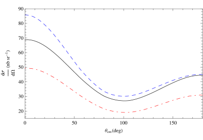
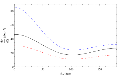
Figure 11: Comparison of differential cross-section calculated at different orders in the c.m. frame. The top two panels are for calculations at 60 MeV (left) and 80 MeV (right) and the bottom two panels are calculations at 100 MeV (left) and 120 MeV (right). The dashed (blue) curves are the ${\mathcal{O}}(e^{2})$ results, the solid (black) curves are the impulse approximation results and the dot-dashed (red) curves are the ${\mathcal{O}}(e^{2}Q)$ results.

In Fig. 11 we plot the dcs for coherent $\gamma\,^{3}$He scattering. For the results reported in this section we employ the ³He  wavefunction obtained using the Idaho chiral $N^{3}LO$ NN potential En03 with the cut-off at 500 MeV together with a chiral three-nucleon interaction No06 . All the different panels are for calculations at different energies (60, 80, 100 and 120 MeV) in the c.m. frame. Each of the panels shows the dcs calculation at different orders– $\mathcal{O}(e^{2})$, Impulse Approximation (IA) and $\mathcal{O}(e^{2}Q)$. Here, Impulse Approximation means that the calculation is done up to ${\mathcal{O}}(e^{2}Q)$ but does not have any two-body contribution– this is not the full $\mathcal{O}(e^{2}Q)$ calculation. As expected, we see that there is a sizeable difference between the IA and the ${\mathcal{O}}(e^{2}Q)$ dcs which means that the two-body currents are important and cannot be neglected. Also, we see that the difference between the $\mathcal{O}(e^{2})$ and $\mathcal{O}(e^{2}Q)$ is very small at 60 MeV and it gradually increases with energy. This can be attributed to the fact that, as energy increases, the energy-dependent contributions from the $A_{1}\ldots A_{6}$ terms increase and this means that there is an opportunity to extract the neutron polarizabilities. At the lowest energy the dcs is still dominated by the proton Thomson term and hence the $\mathcal{O}(e^{2}Q)$ dcs is closest to the $\mathcal{O}(e^{2})$ one, or in other words, $\chi$PT converges well there. Another notable feature is that the $\mathcal{O}(e^{2})$ dcs is independent of the c.m. energy at forward angles, or we can say that the dcs at $\mathcal{O}(e^{2})$ converges to a single value at zero momentum transfer.

Now, focusing just on the $\mathcal{O}(e^{2}Q)$ curves for all four energies it is evident that there is a rapid decrease in the dcs as one goes from 60 MeV to 120 MeV. It remains to be seen whether this drop-off is compensated by addition of the $\Delta$-isobar to the theory. Also notable is the fact that the  ³He Compton scattering dcs is around four times bigger in magnitude compared to deuteron Compton scattering dcs. We conclude that Compton scattering experiments on ³He  are potentially more accurate than on deuteron.

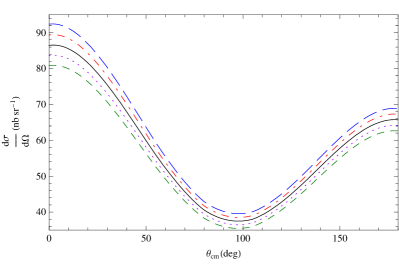
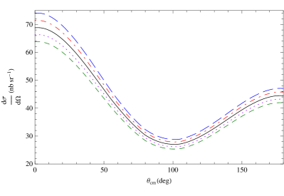
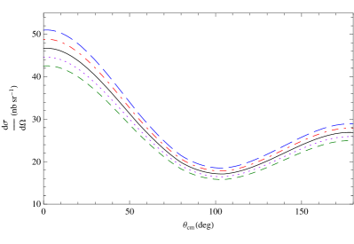
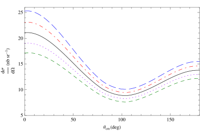
Figure 12: The differential cross-sections in the c.m. frame with varying $\Delta\alpha_{n}$. The top two panels are for calculations at 60 MeV (left) and 80 MeV (right) and the bottom two panels are calculations at 100 MeV (left) and 120 MeV (right). The solid (black) curves correspond to the full $\mathcal{O}(e^{2}Q)$ results. The long-dashed (blue) curves correspond to $\Delta\alpha_{n}=-4\times 10^{-4}$fm³, dot-dashed (red) to $\Delta\alpha_{n}=-2\times 10^{-4}$fm³, dotted (magenta) to $\Delta\alpha_{n}=2\times 10^{-4}$fm³ and dashed (green) to $\Delta\alpha_{n}=4\times 10^{-4}$fm³

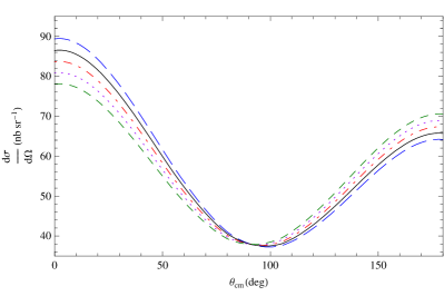
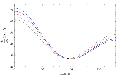
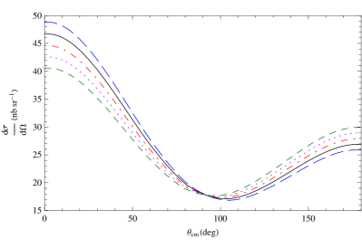
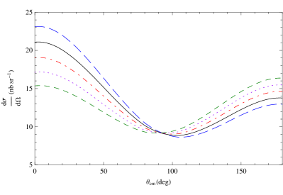
Figure 13: The differential cross-sections in the c.m. frame with varying $\Delta\beta_{n}$. The top two panels are for calculations at 60 MeV (left) and 80 MeV (right) and the bottom two panels are calculations at 100 MeV (left) and 120 MeV (right). The solid (black) curves correspond to the full $\mathcal{O}(e^{2}Q)$ results. The long-dashed (blue) curves correspond to $\Delta\beta_{n}=-2\times 10^{-4}$fm³, dot-dashed (red) to $\Delta\beta_{n}=2\times 10^{-4}$fm³, dotted (magenta) to $\Delta\beta_{n}=4\times 10^{-4}$fm³ and dashed (green) to $\Delta\beta_{n}=6\times 10^{-4}$fm³

Next in Figs. 12 and 13 we plot the $\mathcal{O}(e^{2}Q)$ dcs at different energies by varying $\Delta\alpha_{n}$ and $\Delta\beta_{n}$ respectively. Here we vary $\Delta\alpha_{n}$ between $(-4\ldots 4)\times 10^{-4}$ fm³ and $\Delta\beta_{n}$ between $(-2\ldots 6)\times 10^{-4}$ fm³. (The range of variation of $\Delta\beta_{n}$ is chosen in this manner because of a strong paramagnetic contribution from the $\Delta$-isobar Hi05a ; Hi05 .) What is striking in these figures is that because the ³He  dcs is large compared to that of the deuteron, the sensitivity to $\Delta\alpha_{n}$ and $\Delta\beta_{n}$ is also similarly magnified. It should be evident from the figures that the size of the absolute differences in the dcs as we vary $\Delta\alpha_{n}$ and $\Delta\beta_{n}$ is roughly the same at all energies. However, we would like to advocate that if such measurements were necessary (we expect that $\alpha_{n}$ and $\beta_{n}$ could be determined from ongoing coherent $\gamma d$ experiments at MAXLab at Lund) then it would be better to do them at lowest energy possible. At the lower energies, the dominant contributions come from $\alpha_{n}$ and $\beta_{n}$, apart from the proton Thomson terms. In this regime, we best understand the dynamics and the extraction will not be tainted by contributions from the spin polarizabilities entering via $A_{3}\ldots A_{6}$ and other higher-order contributions. The figures show that even at 60 MeV, the sensitivity to $\alpha_{n}$ and $\beta_{n}$ is sizeable. Another message to take away from these two figures is the beautiful feature in Fig. 13 that sensitivity to ${\beta_{n}}$ vanishes at $\theta=90$ deg and the curves themselves turn over. Thus, in principle one could extract ${\alpha_{n}}$ and ${\beta_{n}}$ independently from the same experiment as opposed to measuring one and then using the sum rule to get the other. A measurement near $\theta=90$ deg would yield ${\alpha_{n}}$ and then one could perform a forward/backward dcs ratio measurement to extract ${\beta_{n}}$. The various curves for $\Delta\alpha_{n}$ suggest that this ratio should not vary much as $\Delta\alpha_{n}$ is varied, but, on the other hand the effect of $\Delta\beta_{n}$ would be magnified compared to what we show in Fig. 13.

In summary, the extraction of ${\alpha_{n}}$ and ${\beta_{n}}$ is possible through coherent Compton scattering on unpolarized $\,{}^{3}$He. Extraction of ${\alpha_{n}}$ and ${\beta_{n}}$ in this manner would also serve as a check for the extractions of ${\alpha_{n}}$ and ${\beta_{n}}$ from the unpolarized $\gamma$d experiments at MAXLab.

V.2 Polarized Compton Scattering

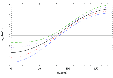
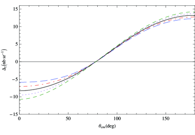
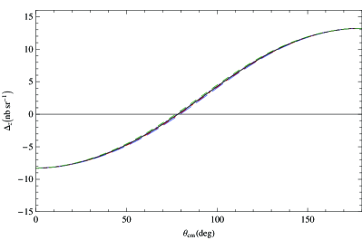
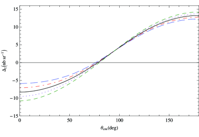
Figure 14: The four panels above correspond to $\Delta_{z}$ with varying each of $\Delta\gamma_{1n}$ (top left), $\Delta\gamma_{2n}$ (top right), $\Delta\gamma_{3n}$ (bottom left) and $\Delta\gamma_{4n}$ (bottom right), one at a time. The calculations are done in c.m. frame at 120 MeV. The solid (black) curves correspond to the full $\mathcal{O}(e^{2}Q)$ results. The long-dashed (blue) curves correspond to $\Delta\gamma_{in}=-\gamma_{in}(\mathcal{O}(e^{2}Q))$, dot-dashed (red) to $\Delta\gamma_{in}=-\gamma_{in}(\mathcal{O}(e^{2}Q))/2$, dotted (magenta) to $\Delta\gamma_{in}=\gamma_{in}(\mathcal{O}(e^{2}Q))/2$ and dashed (green) to $\Delta\gamma_{in}=\gamma_{in}(\mathcal{O}(e^{2}Q))$.

In Fig. 14 we plot $\Delta_{z}$ vs. the c.m. angle at 120 MeV and the different panels correspond to varying the four spin polarizabilities one by one. Here we choose to vary $\gamma_{in},i=1\ldots 4$ between $\pm 100\%$ of their $\mathcal{O}(e^{2}Q)$ prediction (Eqs. (74)). Looking at the plots, the message one gets is that this observable is quite sensitive to $\gamma_{1n}$, $\gamma_{2n}$ and $\gamma_{4n}$. Especially with the expected increase in photon flux at HI$\vec{\gamma}$S such differences in cross-sections should easily be measured and we can expect to extract a linear combination of $\gamma_{1n}$, $\gamma_{2n}$ and $\gamma_{4n}$. The linear combination that readily comes to mind is $\gamma_{0n}$ or $\gamma_{\pi n}$ but we should bear in mind that we are measuring $\Delta_{z}$ as a function of angle which means that we should be able to extract the combination $\gamma_{1n}-(\gamma_{2n}+2\gamma_{4n})\cos\theta$ (see Eq.(73)). Observing the different plots in Fig. 14 we can already see the effect of the $\cos\theta$ term in the panels for $\gamma_{2n}$ and $\gamma_{4n}$.

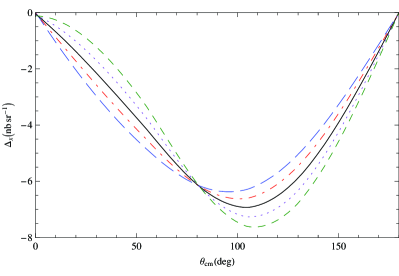
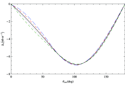
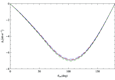
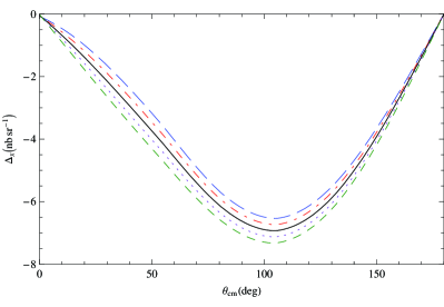
Figure 15: he four panels above correspond to $\Delta_{x}$ with varying each of $\Delta\gamma_{1n}$ (top left), $\Delta\gamma_{2n}$ (top right), $\Delta\gamma_{3n}$ (bottom left) and $\Delta\gamma_{4n}$ (bottom right), one at a time. The calculations are done in c.m. frame at 120 MeV. The solid (black) curves correspond to the full $\mathcal{O}(e^{2}Q)$ results. The long-dashed (blue) curves correspond to $\Delta\gamma_{in}=-\gamma_{in}(\mathcal{O}(e^{2}Q))$, dot-dashed (red) to $\Delta\gamma_{in}=-\gamma_{in}(\mathcal{O}(e^{2}Q))/2$, dotted (magenta) to $\Delta\gamma_{in}=\gamma_{in}(\mathcal{O}(e^{2}Q))/2$ and dashed (green) to $\Delta\gamma_{in}=\gamma_{in}(\mathcal{O}(e^{2}Q))$.

Next, in Fig. 15 we plot $\Delta_{x}$ vs. the c.m. angle at 120 MeV and the different panels correspond to varying the four spin polarizabilities one by one. This figure also suggests that we are sensitive to a combination of the same spin polarizabilities as in $\Delta_{z}$ but this combination is obviously not the same as before $i.e.$ $\gamma_{1n}-(\gamma_{2n}+2\gamma_{4n})\cos\theta$. We can say that because the curves in the right panels of Fig. 15 should coincide at 90 deg because of the $\cos\theta$ term but they do not. Hence, we should be able to extract a different linear combination of the $\gamma_{n}$s from $\Delta_{x}$.

Thus, we are sensitive to two different linear combinations of $\gamma_{1n}$, $\gamma_{2n}$ and $\gamma_{4n}$ through $\Delta_{z}$ and $\Delta_{x}$ and at least we can expect that we can extract one, say $\gamma_{1n}$ unambiguously, out of the three and put constraints on the values of the other two. For $\vec{\gamma}\vec{d}$ scattering we found that we were sensitive to a combination of $\gamma_{1n}$ and $\gamma_{3n}$ Ch05 . This means that if we combine all the information, we should be able to extract at least two of the four spin polarizabilities and constrain the remaining two. Also we can definitely hope that through polarized Compton scattering on deuteron and ³He  we can perform a nuclei independent extraction of at least one of the neutron spin polarizabilities, presumably $\gamma_{1n}$.

It is worth mentioning here that the curves in Figs. 14 and 15 look very similar to those obtained if one calculates the reaction $\vec{\gamma}\vec{n}\rightarrow\gamma n$, i.e. Compton scattering off a free neutron. This would then suggest that polarized ³He  indeed behaves as an “effective” neutron target.

VI Polarized ³He  is Interesting

In this section we would like to point out a couple of very interesting facts about Compton scattering on polarized $\,{}^{3}$He.

1. We know that ³He  is a spin-${1\over 2}$ target and hence, we should be able to write the photon scattering amplitude as a sum of six structure functions like in Eq.(2). However in this case these six functions have to be a sum of one-body and two-body parts and are not as simple as the $A_{i}$s in Eq. (2).

   $$T_{\gamma^{3}He} = \sum\limits_{i=1\ldots 6}A_{i}^{{}^{3}He}t_{i},$$

   $$A_{i}^{{}^{3}He} = A_{i}^{1B}+A_{i}^{2B}.$$ (76)

   Here, $A_{i}^{1B}$ are the same as in Eq.(2) to the extent that ³He is an “effective” neutron. Meanwhile, we found that, numerically, $A_{i}^{2B},i=3\ldots 6$ are negligible. Hence we conclude that $A_{i}^{2B}$ does not contribute to the spin structure functions at $\mathcal{O}(e^{2}Q)$. Moreover, since the two protons (to a good approximation) have spins anti-aligned in a spin-polarized $\,{}^{3}$He target, we can safely assume that all the sensitivity to the spin polarizabilities in the observables come from the unpaired neutron alone. This reasoning supports our claim (made in the previous section) that the curves for ³He  Compton scattering resemble those obtained from $n$-Compton scattering. Thus, Compton scattering on $\,{}^{3}$He is an ideal avenue to extract the neutron spin polarizabilities.

2. Let us consider the double polarization observables, $\Delta_{z}$ and $\Delta_{x}$. If we take Eq. (76) to calculate these observables then we shall obtain expressions similar to Eqs. (3.19) and (3.22) of Ref. mythesis but with $A_{i}$ replaced by $A_{i}^{{}^{3}He}$. From these equations we know that to the lowest order in $\omega$ (${\mathcal{O}}(\omega^{3})$) the spin polarizabilities manifest themselves via the interference terms of $A_{3}\ldots A_{6}$ with $A_{1}$. Hence, to the extent that polarized $\,{}^{3}$He is an effective neutron, we can expect the $A_{3}\ldots A_{6}$ for the neutron will be multiplied by $A_{1}^{{}^{3}He}$, which– at least at low energies– is dominated by the two proton Thomson terms, thus giving a much enhanced effect compared to $\gamma$d.

VII Sources of Uncertainties

VII.1 Wavefunction Dependence

In calculating the matrix elements (Eq. (24)), ideally, the wavefunctions and the operator should be calculated within the same chiral framework, so that the formalism is consistent. Although few-nucleon bound state wavefunctions based on chiral nuclear interactions have been calculated, the currently used approaches are not entirely consistent with the approach used for the Compton scattering operators. Therefore, we employ several wavefunctions based on chiral perturbation theory and additional wavefunction obtained from the state-of-the-art interaction models. In this way we expect to cover the entire dependence on the choice for the wavefunctions. Specifically we chose-

1. The phenomenological potential $AV18$ Wi95 with the $3N$ interaction Urbana IX Pu95 .

2. The Idaho $N^{3}LO$ chiral potential En03 with the cut-off $\Lambda=500$ MeV with a chiral $3N$ force No06 (called $3NFB$ here).

3. The Idaho $N^{3}LO$ chiral potential En03 with the cut-off $\Lambda=500$ MeV with another chiral $3N$ force No06 (called $3NFA$ here). The difference between $3NFA$ and $3NFB$ is that they are parameterized differently so that they reproduce the triton and alpha-particle binding energy but lead to different spectra for heavier nuclei No06 .

4. The Idaho $N^{3}LO$ chiral potential En03 with the cut-off $\Lambda=500$ MeV and no $3NF$.

5. The Idaho $N^{3}LO$ chiral potential En03 with the cut-off $\Lambda=600$ MeV and no $3NF$.

6. The $NLO$ chiral potential with dimensional regularization Ep02 with the cut-off in the Lippman-Schwinger set to $\Lambda=600$ MeV and no $3NF$.

In the future, it will also be interesting to employ wavefunctions based on $NLO$, $N^{2}LO$ and $N^{3}LO$ interactions of Ep05 , which use a different regularization scheme and allow one to compare several orders of the chiral interaction within the one framework. However, we believe that the set of interaction from above should give a reasonable idea of possible wavefunction dependence in this exploratory study. What we want to demonstrate through the choice of these particular wavefunctions is that-

• A contrast between the $NLO$ chiral wavefunction ($\Lambda=600$ MeV) and the Idaho $N^{3}LO$ wavefunction ($\Lambda=600$ MeV) will demonstrate the effect of terms of higher chiral order.

• A contrast between the Idaho $N^{3}LO$ wavefunction ($\Lambda=600$ MeV) without a $3NF$ and the Idaho $N^{3}LO$ wavefunction ($\Lambda=500$ MeV) will demonstrate the effect of varying the cut-off which translates into studying the impact of short-distance physics.

• A contrast between the Idaho $N^{3}LO$ wavefunction ($\Lambda=500$ MeV) and the Idaho $N^{3}LO$ wavefunction ($\Lambda=500$ MeV) with $3NFA$ will demonstrate the effect of ‘a’ three-nucleon force.

• A contrast between the Idaho $N^{3}LO$ wavefunction ($\Lambda=500$ MeV) with $3NFA$ and the Idaho $N^{3}LO$ wavefunction ($\Lambda=500$ MeV) with $3NFB$ will demonstrate the effect of choosing three-nucleon forces with different parameters.

• A contrast between the Idaho $N^{3}LO$ wavefunction ($\Lambda=500$ MeV) with $3NFB$ and the $AV18+$Urbana-IX wavefunction will demonstrate the effect of choosing a wavefunction constructed with a phenomenological potential.

We have calculated the dcs at two different energies (60 & 120 MeV) and also $\Delta_{x}$ and $\Delta_{z}$ at 120 MeV with these six wavefunctions. The results are plotted in Fig. 16.

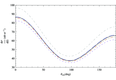
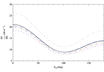
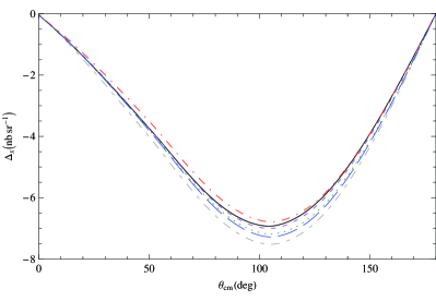
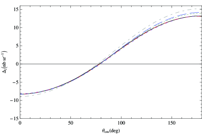
Figure 16: The top two panel show the dcs at 60 MeV (left) and 120 MeV (right) calculated with different wavefunctions. The bottom left panel corresponds to $\Delta_{x}$ at 120 MeV and the bottom right panel corresponds to $\Delta_{z}$ at 120 MeV. These have also been calculated using different wavefunctions. The dashed-shortdashed (grey) curves correspond to $AV18+UrbIX$, solid (black) corresponds to Idaho $N^{3}LO+3NFB$, the long-dashed (blue) curves correspond to Idaho $N^{3}LO+3NFA$, the dot-dashed (red) curves correspond to Idaho $N^{3}LO$ with $\Lambda=500$, the dotted (green) curves correspond to Idaho $N^{3}LO$ with $\Lambda=600$ and the dashed (magenta) curves correspond to $NLO$ chiral wavefunction with $\Lambda=600$. All the calculations have been done in the c.m. frame.

Let us first compare the top two panels that show the dcs. The first thing to notice is that the shape of the dcs is the same no matter what wavefunction we use. Another fact that stands out is that all the chiral potentials produce dcses that are close to one another, whereas the choice of $AV18+$Urbana-IX causes the dcs to be quite different. Also the size of the difference in the dcs due to the choice of different wavefunctions increases as we go from 60 to 120 MeV. One major difference between the chiral wavefunctions and the $AV18+$Urbana-IX wavefunction is that the latter has explicit high-momentum components in the NN interaction and this causes the dcs also to be significantly different. Having said that, it is essential to acknowledge the fact that the dcs is sensitive to the choice of different chiral potentials too. Of these, the chiral wavefunctions with three-nucleon forces and the $N^{3}LO$ chiral wavefunctions are actually of a higher chiral order than our Compton scattering operator and we expect some sensitivity to the higher chiral order terms. Nevertheless, looking at the dcs it can be said that the uncertainty due to the choice of wavefunctions (chiral wavefunctions only) is $\lesssim 15\%$ at 120 MeV. Of course this is lower at 60 MeV ($\lesssim 8\%$) and we advocate that if a measurement of the dcs is necessary to extract $\alpha_{n}$ or $\beta_{n}$ it should be done at lower energies.

Next, observe the lower panels of Fig. 16. What immediately stands out is that even though these calculations were done at 120 MeV, the sensitivity to the choice of wavefunctions is much smaller than in the dcs. This is a good sign because we want to use these double-polarization observables to extract the $\gamma_{n}$s. The uncertainty due to the choice of different wavefunctions in these observables is $\lesssim 7.5\%$. Also, the calculations with the different chiral potentials converge to a single value ($i.e.$ uncertainty is $\sim 0\%$) at forward angles for $\Delta_{z}$ and this augurs well for us because (as we see in Fig. 14) there is maximum sensitivity to the $\gamma_{n}$s at forward angles. Similarly, a measurement of $\Delta_{x}$ at forward angles will also reduce the effect of the wavefunction dependence. But, it should be pointed out that, experimentally, at forward angles there are large background effects and it will be difficult to separate the $\gamma\,^{3}$He scattering events from the background at HI$\vec{\gamma}$S.

VII.2 Position of Pion-production Threshold

In HB$\chi$PT it is assumed that the nucleon rest four momenta dominate their total four momenta, in other words, the nucleons are virtually at rest. In consequence the pion-production threshold occurs at $\omega=m_{\pi}$, because the nucleus cannot recoil. Hence, this assumption creates a problem for all processes involving baryons near the pion-production threshold. The position of the pion-production threshold in $\gamma\,^{3}$He scattering is actually at a photon energy of

$$\omega=-B_{{}^{3}He}+m_{\pi}+\frac{m_{\pi}^{2}}{2M_{{}^{3}He}}+{\mathcal{O}}(m_{\pi}^{3}),$$ (77)

and not at $\omega=m_{\pi}$. Hence, for the purpose of understanding the effect of this in our calculations, we redefined

$$\tilde{\omega}=-B_{{}^{3}He}+\omega+\frac{\omega^{2}}{2M_{{}^{3}He}}$$ (78)

as the energy ‘going into’ the $\gamma N$ amplitude and calculated the dcs at $\omega=$100 MeV. $B_{{}^{3}He}$ is the binding energy of the ³He nucleus in Eq. (78). We found that there was a $\sim 5\%$ difference in the dcs at 100 MeV. In $\Delta_{x}$ the difference was $\sim 1\%$ and in $\Delta_{z}$ the difference was $\sim 3\%$ at 100 MeV. It is encouraging that the percentage uncertainty in the double polarization observables is again less than that in the dcs. This investigation was just exploratory and a proper treatment of this issue is an important topic for future study.

VII.3 Boost Corrections

Our calculation of the $\gamma$³He  scattering process is in the $\gamma{}^{3}$He c.m. frame. However, the one-body amplitude (Eq. (2)) is defined to be in the $\gamma$N c.m. frame and similarly the two-body amplitude is defined to be in the $\gamma$NN c.m. frame. Thus, we need to boost these amplitudes to the $\gamma$NNN c.m. frame. This is necessary to ensure that the vectors ${\hat{\epsilon}}$ and ${\hat{\epsilon}\,^{\prime}}$ stay orthogonal to $\hat{k}$ and ${\hat{k}\,^{\prime}}$ respectively in the new frame. Consequently, a ‘boosting’ term has to be added to the $\gamma$N amplitude which is given by-

$${\hat{O}}_{Boost}^{(1B)} = \frac{e^{2}}{M^{2}\omega}\left[1+{1\over 2}(\tau_{3}^{(1)}+\tau_{3}^{(2)})\right]$$ (79)

$$\left[{1\over 3}\vec{\epsilon}^{\prime}\cdot\vec{k}\,\vec{\epsilon}\cdot\vec{k}^{\prime}+{1\over 2}(\vec{\epsilon}^{\prime}\cdot\vec{p_{3}}\,\vec{\epsilon}\cdot\vec{k}^{\prime}+\vec{\epsilon}\cdot\vec{p_{3}}\,\vec{\epsilon}^{\prime}\cdot\vec{k})\right]$$

$$- {1\over 2}\frac{e^{2}}{M^{2}\omega}(\tau_{3}^{(1)}-\tau_{3}^{(2)})[\vec{\epsilon}^{\prime}\cdot\vec{p_{12}}\,\vec{\epsilon}\cdot\vec{k}^{\prime}+\vec{\epsilon}\cdot\vec{p_{12}}\,\vec{\epsilon}^{\prime}\cdot\vec{k}].$$

Here, all symbols have their usual meanings. The structure of the two-body operator is such that it is Galilean boost invariant. We calculated the effect of this boost at 100 MeV and found that it is truly a perturbative effect and the difference is $\lesssim 0.01\%$ in the dcs. This is because the boost corrections to the transition matrix elements that dominate are really very small if not zero. The boost pieces contribute to those matrix elements that are themselves small and hence play only a small role in the observables.

VIII Summary and Future Prospects

We have performed the first ${\mathcal{O}}(e^{2}Q)$ HB$\chi$PT calculations of Compton scattering on ³He. Indeed we are not aware of any previous theoretical calculation of this reaction process in any framework. We have shown that ³He  Compton scattering is an exciting prospect for mining the neutron polarizabilities. Polarized ³He  is unique and interesting because it does seem to behave as an “effective neutron” (refer to Sec. VI) in Compton scattering. With the added advantage of a significant Compton cross-section due to the presence of the two protons, whose Thomson terms can interfere with the neutron polarizabilities, we get a significantly magnified effect compared to $\gamma$d. The results reported in Sec. V are quite encouraging because they show that not only can we access $\alpha_{n}$ and $\beta_{n}$ through the dcs but we can also hope to extract two different linear combinations of $\gamma_{1n}$, $\gamma_{2n}$ and $\gamma_{4n}$ from the double-polarization observables, $\Delta_{z}$ and $\Delta_{x}$.

Meanwhile, priorities for HI$\vec{\gamma}$S (at Triangle Universities Nuclear laboratory) were discussed at a Compton workshop held prior to the Fifth International Workshop on Chiral Dynamics, 2006 Ha06 and they included polarized $\vec{\gamma}\vec{p}$, $\vec{\gamma}\vec{d}$ and $\vec{\gamma}\vec{{}^{3}He}$ experiments. The idea is that the $\vec{\gamma}\vec{p}\rightarrow\gamma p$ experiments will reveal $\gamma_{1p}\ldots\gamma_{4p}$ and the set for the proton polarizabilities will be complete. This will set the stage for the neutron polarizabilities. Moreover, if the MAXLab experiments generate enough data to extract $\alpha_{n}$ and $\beta_{n}$ unambiguously, then $\gamma{{}^{3}}$He can be used to focus on the neutron spin polarizabilities. One can also hope that coherent  ³He Compton scattering measurements may be done at MAXLab in the future. The expectation is that, at the completion of all these planned experiments we will be able to complete the set of polarizabilities for the neutron.

However, there is a lot of scope for improving the theoretical calculations on ³He  Compton scattering. This being the first calculation was exploratory in nature. Improvements on the theoretical side could include higher-order (${\mathcal{O}}(e^{2}Q^{2})$) calculations and/or explicit inclusion of the $\Delta-$isobar. (We have seen that explicit inclusion of the $\Delta$-isobar causes noticeable changes in the results for $\vec{\gamma}\vec{d}$ scattering.) Also dedicated effort is required to shrink the theoretical uncertainties associated with the choice of nuclear wavefunctions. Hildebrandt $et\,al.$ Hi05b ; Hi05 have demonstrated that by resumming the intermediate NN scattering states they were able to restore the Thomson limit for deuteron Compton scattering and also significantly reduce the dependence on the choice of deuteron wavefunctions. Such an exercise can also be done for ³He  Compton scattering. Effort is also required to rigorously study the effect of the incorrect position of the pion-production threshold due to the “static approximation” for nucleons in HB$\chi$PT . These effects have been studied for $\pi d$ scattering by Baru $et\,al.$ Ba04 and for $\gamma d\rightarrow\pi^{+}nn$ by Lensky $et\,al.$ Le05 . Using similar principles, we can endeavor to resolve this issue for Compton scattering on nuclear targets.

To conclude, it should be reiterated that we have taken the crucial first step. Of course, much needs to be done but we are confident that with sustained efforts we shall be able to extract the neutron polarizabilities from forthcoming $\gamma$³He  scattering data.

Appendix A $\gamma$N Amplitude

After evaluating all the diagrams in Figs. 3 and 4, it becomes evident that the photon scattering amplitude $T_{\gamma N}$ is a sum of six operator structures that can be expressed as:

$$T_{\gamma N} = e^{2}\{A_{1}{\hat{\epsilon}\,^{\prime}}\cdot{\hat{\epsilon}}+A_{2}{\hat{\epsilon}\,^{\prime}}\cdot\hat{k}\,{\hat{\epsilon}}\cdot{\hat{k}\,^{\prime}}+iA_{3}{\vec{\sigma}}\cdot({\hat{\epsilon}\,^{\prime}}\times{\hat{\epsilon}})$$ (1)

$$+iA_{4}{\vec{\sigma}}\cdot({\hat{k}\,^{\prime}}\times\hat{k})\,{\hat{\epsilon}\,^{\prime}}\cdot{\hat{\epsilon}}+iA_{5}{\vec{\sigma}}\cdot[({\hat{\epsilon}\,^{\prime}}\times\hat{k})\,{\hat{\epsilon}}\cdot{\hat{k}\,^{\prime}}-({\hat{\epsilon}}\times{\hat{k}\,^{\prime}})\,{\hat{\epsilon}\,^{\prime}}\cdot\hat{k}]$$

$$+iA_{6}{\vec{\sigma}}\cdot[({\hat{\epsilon}\,^{\prime}}\times{\hat{k}\,^{\prime}})\,{\hat{\epsilon}}\cdot{\hat{k}\,^{\prime}}-({\hat{\epsilon}}\times\hat{k})\,{\hat{\epsilon}\,^{\prime}}\cdot\hat{k}]\}$$

$$= \sum_{i=1}^{6}A_{i}t_{i}$$ (2)

where,

$$t_{1} = e^{2}{\hat{\epsilon}\,^{\prime}}\cdot{\hat{\epsilon}}$$

$$t_{1} = e^{2}{\hat{\epsilon}\,^{\prime}}\cdot\hat{k}\,{\hat{\epsilon}}\cdot{\hat{k}\,^{\prime}}$$

$$t_{1} = ie^{2}{\vec{\sigma}}\cdot({\hat{\epsilon}\,^{\prime}}\times{\hat{\epsilon}})$$

$$t_{1} = ie^{2}{\vec{\sigma}}\cdot({\hat{k}\,^{\prime}}\times\hat{k})\,{\hat{\epsilon}\,^{\prime}}\cdot{\hat{\epsilon}}$$

$$t_{1} = ie^{2}{\vec{\sigma}}\cdot[({\hat{\epsilon}\,^{\prime}}\times\hat{k})\,{\hat{\epsilon}}\cdot{\hat{k}\,^{\prime}}-({\hat{\epsilon}}\times{\hat{k}\,^{\prime}})\,{\hat{\epsilon}\,^{\prime}}\cdot\hat{k}]$$

$$t_{6} = ie^{2}{\vec{\sigma}}\cdot[({\hat{\epsilon}\,^{\prime}}\times{\hat{k}\,^{\prime}})\,{\hat{\epsilon}}\cdot{\hat{k}\,^{\prime}}-({\hat{\epsilon}}\times\hat{k})\,{\hat{\epsilon}\,^{\prime}}\cdot\hat{k}]$$

The six invariant amplitudes, $A_{1}\ldots A_{6}$, are functions of the photon energy, $\omega$, and the Mandelstam variable $t$. Defining $\Upsilon=\omega/m_{\pi}$ and $t=-2{\Upsilon^{2}}(1-\cos\theta)$, where $\theta$ is the center-of-mass angle between the incoming and outgoing photon momenta, one finds bkmrev ; Be91 ; Be92 ; Be93 ; Be94 :

$$A_{1} = -\frac{{\mathcal{Z}}^{2}}{M}+\frac{g_{A}^{2}m_{\pi}}{8\pi f_{\pi}^{2}}\left\{1-\sqrt{1-\Upsilon^{2}}+\frac{2-t}{\sqrt{-t}}\left[\frac{1}{2}\arctan\frac{\sqrt{-t}}{2}-I_{1}(\Upsilon,t)\right]\right\},$$

$$A_{2} = \frac{{\mathcal{Z}}^{2}\omega}{M^{2}}-\frac{g_{A}^{2}\omega^{2}}{8\pi f_{\pi}^{2}m_{\pi}}\frac{2-t}{(-t)^{3/2}}\left[I_{1}(\Upsilon,t)-I_{2}(\Upsilon,t)\right],$$

$$A_{3} = \frac{\omega}{2M^{2}}[{\mathcal{Z}}({\mathcal{Z}}+2\kappa)-({\mathcal{Z}}+\kappa)^{2}\cos\theta]+\frac{{(2{\mathcal{Z}}-1)}g_{A}m_{\pi}}{8\pi^{2}f_{\pi}^{2}}\frac{\Upsilon t}{1-t}$$

$$+\frac{g_{A}^{2}m_{\pi}}{8\pi^{2}f_{\pi}^{2}}\left[\frac{1}{\Upsilon}\arcsin^{2}\Upsilon-\Upsilon+2\Upsilon^{4}\sin^{2}\theta I_{3}(\Upsilon,t)\right],$$

$$A_{4} = -\frac{({\mathcal{Z}}+\kappa)^{2}\omega}{2M^{2}}+\frac{g_{A}^{2}\omega^{2}}{4\pi^{2}f_{\pi}^{2}m_{\pi}}I_{4}(\Upsilon,t),$$

$$A_{5} = \frac{({\mathcal{Z}}+\kappa)^{2}\omega}{2M^{2}}-\frac{{(2{\mathcal{Z}}-1)}g_{A}\omega^{2}}{8\pi^{2}f_{\pi}^{2}m_{\pi}}\frac{\Upsilon}{(1-t)}-\frac{g_{A}^{2}\omega^{2}}{8\pi^{2}f_{\pi}^{2}m_{\pi}}[I_{5}(\Upsilon,t)-2\Upsilon^{2}\cos\theta I_{3}(\Upsilon,t)],$$

$$A_{6} = -\frac{{\mathcal{Z}}({\mathcal{Z}}+\kappa)\omega}{2M^{2}}+\frac{{(2{\mathcal{Z}}-1)}g_{A}\omega^{2}}{8\pi^{2}f_{\pi}^{2}m_{\pi}}\frac{\Upsilon}{(1-t)}$$ (4)

$$+\frac{g_{A}^{2}\omega^{2}}{8\pi^{2}f_{\pi}^{2}m_{\pi}}[I_{5}(\Upsilon,t)-2\Upsilon^{2}I_{3}(\Upsilon,t)],$$

where ${\mathcal{Z}}=1$(0) for the proton(neutron) and:

$$I_{1}(\Upsilon,t) = \int_{0}^{1}dz\,\arctan\frac{(1-z)\sqrt{-t}}{2\sqrt{1-\Upsilon^{2}z^{2}}},$$

$$I_{2}(\Upsilon,t) = \int_{0}^{1}dz\,\frac{2(1-z)\sqrt{-t(1-\Upsilon^{2}z^{2})}}{4(1-\Upsilon^{2}z^{2})-t(1-z)^{2}},$$

$$I_{3}(\Upsilon,t) = \int_{0}^{1}dx\,\int_{0}^{1}dz\,\frac{x(1-x)z(1-z)^{3}}{S^{3}}\left[\arcsin\frac{\Upsilon z}{R}+\frac{\Upsilon zS}{R^{2}}\right],$$

$$I_{4}(\Upsilon,t) = \int_{0}^{1}dx\,\int_{0}^{1}dz\,\frac{z(1-z)}{S}\arcsin\frac{\Upsilon z}{R},$$

$$I_{5}(\Upsilon,t) = \int_{0}^{1}dx\,\int_{0}^{1}dz\,\frac{(1-z)^{2}}{S}\arcsin\frac{\Upsilon z}{R},$$ (5)

with

$$S=\sqrt{1-\Upsilon^{2}z^{2}-t(1-z)^{2}x(1-x)},\qquad R=\sqrt{1-t(1-z)^{2}x(1-x)}.$$ (6)

Appendix B $\gamma$NN Amplitude

The two-body diagrams that contribute to the Compton scattering process at ${\mathcal{O}}(e^{2}Q)$ are shown in Fig. 5. The two-body amplitude can be expressed (in the $\gamma$NN c.m. frame) Be99 ; Be02 ; Be04 as:

$$T_{\gamma NN}^{2B}\;=\;-\frac{{e^{2}}{g_{A}^{2}}}{2f_{\pi}^{2}}\;({\vec{\tau}}^{\;1}\cdot{\vec{\tau}}^{\;2}-\tau^{1}_{3}\tau^{2}_{3})\;(t^{(a)}+t^{(b)}+t^{(c)}+t^{(d)}+t^{(e)}),$$ (1)

where

$${t^{(a)}} = \frac{{{\hat{\epsilon}}\cdot{\vec{\sigma}^{\scriptscriptstyle 1}}}\;{{\hat{\epsilon}\,^{\prime}}\cdot{\vec{\sigma}^{\scriptscriptstyle 2}}}}{2[{\omega^{2}}-{m_{\pi}^{2}}-({\vec{p}}-{{\vec{p}}\,^{\prime}}+{\frac{1}{2}({\vec{k}}+{{\vec{k}}\,^{\prime}})})^{2}]}+(1\;\leftrightarrow\;2),$$ (2)

$${t^{(b)}} = \frac{{{\hat{\epsilon}}\cdot{\hat{\epsilon}\,^{\prime}}}\;{\vec{\sigma}^{\scriptscriptstyle 1}}\cdot({\vec{p}}-{{\vec{p}}\,^{\prime}}-{\frac{1}{2}({\vec{k}}-{{\vec{k}}\,^{\prime}})}){\vec{\sigma}^{\scriptscriptstyle 2}}\cdot({\vec{p}}-{{\vec{p}}\,^{\prime}}+{\frac{1}{2}({\vec{k}}-{{\vec{k}}\,^{\prime}})})}{2[({\vec{p}}-{{\vec{p}}\,^{\prime}}-{\frac{1}{2}({\vec{k}}-{{\vec{k}}\,^{\prime}})})^{2}+{m_{\pi}^{2}}][({\vec{p}}-{{\vec{p}}\,^{\prime}}+{\frac{1}{2}({\vec{k}}-{{\vec{k}}\,^{\prime}})})^{2}+{m_{\pi}^{2}}]}$$ (3)

$$+ (1\;\leftrightarrow\;2),$$

$${t^{(c)}} = -\frac{{{\hat{\epsilon}\,^{\prime}}\cdot({\vec{p}}-{{\vec{p}}\,^{\prime}}+{\frac{1}{2}{\vec{k}}})}\;{\vec{\sigma}^{\scriptscriptstyle 1}}\cdot{\hat{\epsilon}}\;{\vec{\sigma}^{\scriptscriptstyle 2}}\cdot({\vec{p}}-{{\vec{p}}\,^{\prime}}+{\frac{1}{2}({\vec{k}}-{{\vec{k}}\,^{\prime}})})}{[{\omega^{2}}-{m_{\pi}^{2}}-({\vec{p}}-{{\vec{p}}\,^{\prime}}+{\frac{1}{2}({\vec{k}}+{{\vec{k}}\,^{\prime}})})^{2}][({\vec{p}}-{{\vec{p}}\,^{\prime}}+{\frac{1}{2}({\vec{k}}-{{\vec{k}}\,^{\prime}})})^{2}+{m_{\pi}^{2}}]}$$ (4)

$$+ (1\;\leftrightarrow\;2),$$

$${t^{(d)}} = -\frac{{{\hat{\epsilon}}\cdot({\vec{p}}-{{\vec{p}}\,^{\prime}}+{\frac{1}{2}{{\vec{k}}\,^{\prime}}})}\;{\vec{\sigma}^{\scriptscriptstyle 1}}\cdot({\vec{p}}-{{\vec{p}}\,^{\prime}}-{\frac{1}{2}({\vec{k}}-{{\vec{k}}\,^{\prime}})}){\vec{\sigma}^{\scriptscriptstyle 2}}\cdot{\hat{\epsilon}\,^{\prime}}}{[{\omega^{2}}-{m_{\pi}^{2}}-({\vec{p}}-{{\vec{p}}\,^{\prime}}+{\frac{1}{2}({\vec{k}}+{{\vec{k}}\,^{\prime}})})^{2}][({\vec{p}}-{{\vec{p}}\,^{\prime}}-{\frac{1}{2}({\vec{k}}-{{\vec{k}}\,^{\prime}})})^{2}+{m_{\pi}^{2}}]}$$ (5)

$$+ (1\;\leftrightarrow\;2),$$

$${t^{(e)}} = \frac{2{{\hat{\epsilon}}\cdot({\vec{p}}-{{\vec{p}}\,^{\prime}}+{\frac{1}{2}{{\vec{k}}\,^{\prime}}})\;{\hat{\epsilon}\,^{\prime}}\cdot({\vec{p}}-{{\vec{p}}\,^{\prime}}+{\frac{1}{2}{\vec{k}}})}\;{\vec{\sigma}^{\scriptscriptstyle 1}}\cdot({\vec{p}}-{{\vec{p}}\,^{\prime}}-{\frac{1}{2}({\vec{k}}-{{\vec{k}}\,^{\prime}})})\;}{[{\omega^{2}}-{m_{\pi}^{2}}-({\vec{p}}-{{\vec{p}}\,^{\prime}}+{\frac{1}{2}({\vec{k}}+{{\vec{k}}\,^{\prime}})})^{2}][({\vec{p}}-{{\vec{p}}\,^{\prime}}-{\frac{1}{2}({\vec{k}}-{{\vec{k}}\,^{\prime}})})^{2}+{m_{\pi}^{2}}]}$$ (6)

$$\times \frac{{\vec{\sigma}^{\scriptscriptstyle 2}}\cdot({\vec{p}}-{{\vec{p}}\,^{\prime}}+{\frac{1}{2}({\vec{k}}-{{\vec{k}}\,^{\prime}})})}{[({\vec{p}}-{{\vec{p}}\,^{\prime}}+{\frac{1}{2}({\vec{k}}-{{\vec{k}}\,^{\prime}})})^{2}+{m_{\pi}^{2}}]}+(1\;\leftrightarrow\;2),$$

Here again, ${\hat{\epsilon}},{\hat{\epsilon}\,^{\prime}},{\vec{k}},{{\vec{k}}\,^{\prime}}$ have their usual meaning. ${\vec{p}}$(${{\vec{p}}\,^{\prime}}$) is the initial (final) momentum of the nucleon inside the deuteron, and ${\vec{\sigma}^{\scriptscriptstyle 1}}$(${\vec{\sigma}^{\scriptscriptstyle 2}}$) is twice the spin operator of the first (second) nucleon. The numbering of the nucleons is arbitrary and hence ($1\leftrightarrow 2$) denotes the term when the nucleons are interchanged.

References

- (1) B. R. Holstein, D. Drechsel, B. Pasquini, M. Vanderhaeghen, Phys. Rev. C61, 034316 (2000).
- (2) D. Babusci, G. Giordano and G. Matone, Phys. Rev. C57, 291–294 (1998).
- (3) S. Ragusa, Phys. Rev. D47, 3757 (1993).
- (4) M. Bawin, and S. A. Coon, Phys. Rev. C55, 419 (1997).
- (5) F. J. Federspiel et al. Phys. Rev. Lett. 67, 1511–1514 (1991).
- (6) A. Zieger Phys. Lett. B278, 34–38 (1992).
- (7) E. L. Hallin et al. Phys. Rev. C48(4), 1497–1507 (1993).
- (8) B. E. MacGibbon et al. Phys. Rev. C52(4), 2097–2109 (1995).
- (9) V. Olmos de Leon et al. Eur. Phys. J. A10, 207–215 (2001).
- (10) R. A. Arndt, I. I. Strakovsky and R. L. Workman, Phys. Rev. C53(1), 430–440 (1996).
- (11) A. I. L’vov, V. A. Petrun’kin and M. Schumacher, Phys. Rev. C55(1), 359–377 (1997).
- (12) J. A. McGovern, Phys. Rev. C63, 064608 (2001).
- (13) S. R. Beane, M. Malheiro, J. A. McGovern, D. R. Phillips, and U. van Kolck, Phys. Lett B567, 200 (2003). Erratum-ibid: Phys. Lett. B607 320 (2005).
- (14) S. R. Beane, M. Malheiro, J. A. McGovern, D. R. Phillips, and U. van Kolck, Nucl. Phys. A747, 311–361 (2005).
- (15) V. Bernard, N. Kaiser, and Ulf-G. Meißner, Int. J. Mod. Phys. E4, 193 (1995).
- (16) A. I. L’vov, V. A. Petrunkin and S. A. Startsev, Yad. Fiz. 29, 1265 (1979) [Sov. J. Nucl. Phys. 29 651 (1979)]; U. E. Schrder, Nucl. Phys. B166 103 (1980).
- (17) M. I. Levchuk and A. I. L’vov, Nucl. Phys. A674, 449–492 (2000).
- (18) J. Schmiedmayer, P. Riehs, J. A. Harvey and N. W. Hill, Phys. Rev. Lett., 66, 1015–1018 (1991).
- (19) L. Koester, W. Waschkowski, L. V. Mitsyna, G. S. Samosvat, P. Prokofjevs and J. Tambergs, Phys. Rev. C51, 3363–3371 (1995).
- (20) T. L. Enik, L. V. Mitsyna, V. G. Nikolenko, A. B. Popov and G. S. Samosvat, Phys. Atom. Nucl. 60, 567–570 (1997).
- (21) N. R. Kolb, A. W. Rauf, R. Igarashi, D. L. Hornidge, R. E. Pywell, B. J. Warkentin, E. Korkmaz, G. Feldman, and G. V. O’Rielly, Phys. Rev. Lett. 85, 1388–1391 (2000).
- (22) K. Kossert et al. Eur. Phys. J. A16, 259–273 (2003).
- (23) M. Camen, et al. Phys. Rev. C65, 032202 (2002).
- (24) G. Galler, et al. Phys. Lett. B503, 245–255 (2001).
- (25) S. Wolf, et al. Eur. Phys. J. A12, 231–252 (2001).
- (26) T. R. Hemmert, B. R., Holstein, J. Kambor, and G. Knöchlein, Phys. Rev. D57(9), 5746–5754 (1998).
- (27) V. Pascalutsa, and D. R. Phillips, Phys. Rev. C68, 055205 (2003).
- (28) M. Gell-Mann, M. L. Goldberger and W. E. Thirring, Phys. Rev. 95, 1612 (1954).
- (29) A. M. Sandorfi, M. Khandaker, and C. S. Whisnant, Phys. Rev. D50, R6681 (1994).
- (30) M. Weyrauch and H. Arenhövel, Nucl. Phys. A408, 425–460 (1983).
- (31) T. Wilbois, P. Wilhelm, and H. Arenhövel, Few Body Sys. Suppl. 9, 263–266 (1995).
- (32) M. I. Levchuk, and A. I. L’vov, Few Body Sys. Suppl. 9, 239 (1995).
- (33) M. I. Levchuk, and A. I. L’vov, arXiv.org:nucl-th/9809034 (1998).
- (34) J. J. Karakowski, and G. A. Miller, Phys. Rev. C60, 014001 (1999).
- (35) R. P. Hildebrandt, H. W. Grießhammer, T. R. Hemmert, and D. R. Phillips, Nucl. Phys., A748, 573 (2005).
- (36) R. P. Hildebrandt, H. W. Grießhammer, and T. R. Hemmert, nucl-th/0512063 (2005).
- (37) R. P. Hildebrandt, Ph. D. Thesis, arXiv.org:nucl-th/0512064.
- (38) R. P. Hildebrandt, H. W. Griesshammer, and T. R. Hemmert, Eur. Phys. J. A20, 329 (2004).
- (39) D. Choudhury, and D. R. Phillips, Phys. Rev., C71, 044002 (2005).
- (40) D. Choudhury, Ph.D. Thesis, (2006).
- (41) D. Shukla, and H. W. Grießhammer (in preparation).
- (42) S. R. Beane, M. Malheiro, D. R. Phillips, and U. van Kolck, Nucl. Phys. A656, 367–399 (1999).
- (43) B. Blankleider and R. M. Woloshyn, Phys. Rev., C29, 538 (1984); J. L. Friar et al., Phys. Rev., C42, 2310 (1990).
- (44) A. Nogga, et al., Phys. Rev. C67, 034004 (2003).
- (45) D. Choudhury, A. Nogga and D. R. Phillips, Phys. Rev. Lett. 98 232303 (2007); D. Choudhury, D. R. Phillips and A. Nogga, 5th International Workshop on Chiral Dynamics, Theory and Experiment, published in the proceedings (World Scientific, Singapore, 2007).
- (46) A. Nogga, et al., Phys. Lett. B409, 19 (1997).
- (47) V. V. Kotlyar, H. Kamada, J. Golak and W. Glöckle, Few-Body Systems 28, 35 (2000).
- (48) E. Epelbaum, W. Glöckle, A. Krüger, and U.-G. Meißner, Nucl. Phys. A645, 413 (1999).
- (49) E. Epelbaum, W. Glöckle, and U.-G. Meißner, Nucl. Phys. A671, 295 (2000).
- (50) D. R. Entem and R. Machleidt, Phys. Rev., C68, 041001 (2003).
- (51) R. B. Wiringa, V. G. J. Stoks, and R. Schiavilla, Phys. Rev. C51, 38 (1995).
- (52) U. van Kolck, Phys. Rev., C49, 2932 (1994); A., Nogga, P., Navratil, B. R., Barrett, and J. P. Vary, Phys. Rev. C73, 064002 (2006).
- (53) B. S., Pudliner, V. R., Pandharipande, J., Carlson, and R. B. Wiringa, Phys. Rev. Lett. 74, 4396 (1995).
- (54) E. Epelbaum, et al., Eur. Phys. J. A15, 543(2002).
- (55) E. Epelbaum, et al., Nucl. Phys. A747, 362 (2005).
- (56) H-W. Hammer, N. Kalantar, and D. R. Phillips, 5th International Workshop on Chiral Dynamics, Theory and Experiment, published in the proceedings (World Scientific, Singapore, 2007).
- (57) V. Baru, C. Hanhart, A. E. Kudryavtsev, and U. G. Meißner, Phys. Lett. B589, 118 (2004).
- (58) V. Lensky, et al. Eur. Phys. J. A26, 107 (2005).
- (59) V. Bernard, N. Kaiser, and Ulf-G. Meißner, Phys. Rev. Lett. 67, 1515 (1991).
- (60) V. Bernard, N. Kaiser, J. Kambor and Ulf-G. Meißner, Nuc. Phys. B388, 315 (1992).
- (61) V. Bernard, N. Kaiser, A. Schmidt and Ulf-G. Meißner, Phys. Lett. B319, 269 (1993).
- (62) V. Bernard, N. Kaiser, Ulf-G. Meißner and A. Schmidt, Z. Phys. A348, 317 (1994).