Optical vortex soliton with self-defocusing Kerr-type nonlocal nonlinearity

Abstract

We develop one numerical method to compute the optical vortex soliton with self-defocusing Kerr-type nonlocal nonlinearity. With the numerical simulation method, the propagation and interaction properties of such optical vortex solitons are investigated.

I Introduction

Optical vortex solitons are self trapped intensity dips with screw phase dislocations. Owing to such screw phase dislocations, there is one phase singular point of the vortex whose real and imaginary parts both vanish. Circumnavigating the phase singular point in a counterclockwise direction a $\pm 2m\pi$ phase ramp is picked up. The integer $\pm m$ is called a topological charge of the vortex. Optical vortex solitons can be generated in self-defocusing nonlinear medium as consequences of the counterbalanced effect of diffraction and nonlinearity of the medium. The numerical forms or approximate forms of the vortices are investigated14 ; 15 ; 16 . Optical vortices have been observed in a Kerr type nonlinear medium1 , in a photorefractive crystal2 and in a saturable nonlinear medium3 ; 4 . The stability of two dimensional vortices and one dimensional dark solitons are investigated2 ; 4 ; 5 ; 6 ; 7 ; 8 ; 9 ; 13 ; 15 . It is indicated that one-dimensional dark soliton stripes can decay into optical vortex solitons due to transverse modulation instability5 ; 6 ; 9 . A vortex of charge $|m|>1$ is found to be topologically unstable and will split into $|m|$ singly charged vortices under perturbations with the total charge conserved2 ; 7 . Hight order screw dislocation ($|m|>1$) are very sensitive to perturbations7 . However if the perturbation is very small, these resulted singly charged vortices will locate too close to be distinguished, and in this case the splitting multicharged vortex is still viewed as a whole one formed as these nearly superposed singly charged vortices. It is indicated that multicharged vortices are very long-living objects and called to be metastable8 . The rotation of a pair of first-order screw dislocation with equal signs and annihilation of a pair of dislocations of opposite signs were detected7 ; 10 . In the limit that the interval distances between vortices are much larger than the size of the core of the vortices, the vortices can be viewed as point vortices11 ; 12 . Interestingly upon breakup of the input high-charge vortex the resulting charge-one vortices repel each other and form an array aligned perpendicular to the anisotropy axis of photorefractive crystal2 .

In this paper, We develop one numerical method to compute the optical vortex soliton with self-defocusing Kerr-type nonlocal nonlinearity. Such numerical method is similar to those presented in reference17 ; 18 ; 19 . With the numerical simulation method, the propagation and interaction properties of such optical vortex solitons are investigated.

II Numerical method to compute nonlocal vortex soltions

The propagation of an optical beam in spatially nonlocal self-defocusing media can be described by this following (1+2) dimensional nonlocal nonlinear Schödinger equation(NNLSE)

$$i{{\partial u}\over{\partial z}}+{{1}\over{2}}\nabla_{\bot}^{2}u-u\int R(|\textbf{r}-\textbf{r}^{\prime}|)|u(\textbf{r}^{\prime},z)|^{2}d^{2}\textbf{r}^{\prime}=0$$ (1)

where $u(\textbf{r},z)$ is the complex amplitude envelop of the light beam, $|u(\textbf{r},z)|^{2}$ is the light intensity, $\textbf{r}=x\hat{\textbf{x}}+y\hat{\textbf{y}}$ and $z$ are transverse and longitude coordinates respectively, $\nabla_{\bot}^{2}={{\partial^{2}}\over{\partial x^{2}}}+{{\partial^{2}}\over{\partial y^{2}}}$ is the transverse Laplace operator. $R(|\textbf{r}|),(\int R(|\textbf{r}|)d^{2}\textbf{r}=1)$ is the real axisymmetric nonlocal response function, and $n(\textbf{r},z)=-\int R(|\textbf{r}-\textbf{r}^{\prime}|)|u(\textbf{r}^{\prime},z)|^{2}d^{2}\textbf{r}^{\prime}$ is the light-induced perturbed refractive index. Note that not stated otherwise all integrals in this paper will extend over the whole transverse x-y plane. When $R(|\textbf{r}|)=\delta(x,y)$, equation (1) will reduce to the local nonlinear Schödinger equation(NLSE)

$$i{\partial u\over\partial z}+{{1}\over{2}}\nabla_{\bot}^{2}u-|u|^{2}u=0,$$ (2)

which has vortex soliton solutions in the form of3 ; 8 ; 11

$$u(\textbf{r},z)=F(r)e^{i\beta z+im\varphi}=\Psi(r,\varphi)e^{i\beta z},$$ (3)

where $\beta^{*}=\beta$ is the phase constant, $\varphi$ is the azimuthal angle, $m=\pm 1,\pm 2,\cdots$ is the topology charge, $F^{*}(r)=F(r)$, $F(0)=0$ and $F(r)\rightarrow\rm{const}=\eta$ as $r\rightarrow\infty$.

In this paper we numerically compute the vortex soliton solutions of NNLSE (1) expressed in the form of Eq. (3). Substituting Eq. (3) into (1) and considering the asymptotic behavior under $r\rightarrow\infty$, we have $\beta=-\eta^{2}$. Then we have

$$\eta^{2}\Psi+{{1}\over{2}}\nabla_{\bot}^{2}\Psi-\Psi\int R(|\textbf{r}-\textbf{r}^{\prime}|)|\Psi(\textbf{r}^{\prime})|^{2}d^{2}\textbf{r}^{\prime}=0$$ (4)

We discrete the function $\Psi(x,y)$ in $\Psi_{jk}=\Psi\big{(}-h+(j-1)\triangle x,-h+(k-1)\triangle y\big{)}$, where $-h<x<h,-h<y<h$ is the sample window, $\triangle x=\triangle y$ is the sample step. Define the discrete Fourier transform (DFT) $\mathscr{F}$ by

$$\widetilde{\Psi}_{jk}=\mathscr{F}[\Psi]_{jk}=\sum_{p,q=1}^{n}\rm{F}_{jp}\Psi_{pq}\rm{F}_{qk}$$ (5a)

$$\Psi_{jk}=\mathscr{F}^{-1}[\widetilde{\Psi}]_{jk}=\sum_{p,q=1}^{n}\rm{F}^{*}_{jp}\widetilde{\Psi}_{pq}\rm{F}^{*}_{qk}$$ (5b)

where $\rm{F}_{jk}={{1}\over{\sqrt{n}}}\exp[i{{2\pi}\over{n}}(j-1)(k-1)]$ and $n={{2h}\over{\triangle x}}+1$. Taking the DFT on Eq. (4),we have

$$\eta^{2}\widetilde{\Psi}_{jk}-{{1}\over{2}}\Omega_{jk}\widetilde{\Psi}_{jk}$$

$$-\mathscr{F}\left[\Psi\int R(|\textbf{r}-\textbf{r}^{\prime}|)|\Psi(\textbf{r}^{\prime})|^{2}d^{2}\textbf{r}^{\prime}\right]_{jk}=0$$ (6)

where $\Omega_{jk}=\left({{2\sin[{{\pi}\over{n}}(j-1)]}\over{\triangle x}}\right)^{2}+\left({{2\sin[{{\pi}\over{n}}(k-1)]}\over{\triangle y}}\right)^{2}$. From Eq. (II), we obtain

$$\widetilde{\Psi}_{jk} ={{(\mu+\eta^{2})\widetilde{\Psi}_{jk}-\mathscr{F}\left[\Psi\int R(|\textbf{r}-\textbf{r}^{\prime}|)|\Psi(\textbf{r}^{\prime})|^{2}d^{2}\textbf{r}^{\prime}\right]_{jk}}\over{\mu+{{1}\over{2}}\Omega_{jk}}}$$ (7)

$$\equiv\mathscr{D}[\Psi]_{jk}$$

where $\mu$ is an arbitrary positive constant.

We use Eq. (7) to iteratively compute the vortex soliton solutions. For an initial trying function, for instance,

$$\Psi_{0}(r,\varphi)=\eta\left[1-\exp\left(-{{r^{m}}\over{\sigma^{m}}}\right)\right]\exp(im\varphi),$$ (8)

where $\sigma$ is a constant, from Eq. (7), we get $\widetilde{\Psi}_{1}=\mathscr{D}[\Psi_{0}]$ and $\Psi_{1}=\mathscr{F}^{-1}[\widetilde{\Psi}_{1}]$. For $p\geq 1$, we get the iteration scheme $\widetilde{\Psi}_{p+1}=\mathscr{D}[\Psi_{p}]$ and $\Psi_{p+1}=\mathscr{F}^{-1}[\widetilde{\Psi}_{p+1}]$. Perform the iteration until some accuracy is achieved, then we get the approximate numerical vortex soliton solutions.

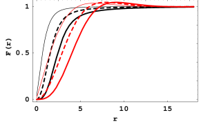
Figure 1: Modulus of vortex’ amplitude $F(r)$ with $F(\infty)=\eta=1$:thin solid dark line corresponds to local case $w=0$ and charge $m=1$; thin solid red line $w=6,m=1$; dashing dark line $w=0,m=2$; dashing red line $w=6,m=2$; thick solid dark line $w=0,m=3$; thick solid red line $w=6,m=3$.

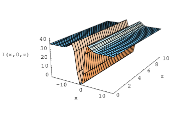
Figure 2: Intensity $I(x,0,z)$ on plane $y=0$ of vortex of charge $m=2$ obtained by numerical simulation with parameters $\eta=6,w=10$.

As an example, we consider this following nonlocal case in which the light-induced perturbed refractive index is governed by

$$n-w^{2}\nabla^{2}_{\bot}n=-|u|^{2},$$ (9)

which results in

$$n(\vec{r},z)={{1}\over{2\pi w^{2}}}\int\rm{K}_{0}\left({{|\vec{r}-\vec{\rho}|}\over{w}}\right)|u(\vec{\rho},z)|^{2}d^{2}\vec{\rho},$$ (10)

where $\rm{K}_{0}(x)$ is the modified Bessel function of the second kind and $w$ is the characteristic nonlocal length. As indicated in Fig. (1), the cores of vortices of the same topology charge and the same background intensity increase with the increasing of characteristic nonlocal length. The numerical simulation shown in Fig. (2) indicates that the numerical solution of vortices obtained by our method can describe the vortices very well. As shown in Fig. (2) there is no observable splitting of the vortex of charge $m=2$ with absence of perturbations during the numerical simulation length $z=10$. It is consistent with the statement that multicharged vortices are metastable8 .

To numerically investigate the stability of singly charged vortex, we use an input vortex with half of the core size of the corresponding vortex soliton, that is

$$u(r,\varphi,0)=F(2r)\exp(i\varphi),$$ (11)

where $F(r)$ is the modulus of the corresponding vortex soliton’s amplitude. The simulation results are shown in Fig. (3), from which we can find the initially shrunk singly charged vortex will evolve to the corresponding vortex soliton along with radiation of ripples. So it is numerically implies that singly charged vortex is stable.

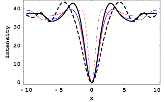
Figure 3: Intensity profiles on plane $y=0$ of the evolving singly charged vortex with an initially shrunk core size. Dashing red line corresponds to input intensity of input beam with half of the core size of the corresponding vortex soliton; Dashing dark line corresponds to intensity at $z=3.3$; Solid dark line $z=8.7$; Blue line $z=17.5$. The solid red line is the intensity of the corresponding singly charged vortex soliton. The simulation parameters are $m=1,\eta=6,w=10$.

In another case we consider this following initial amplitude

$$u(x,y,0) =\left[1-e^{-{{(x-d/2)^{2}+y^{2}}\over{2}}}-e^{-{{(x+d/2)^{2}+y^{2}}\over{2}}}\right]$$ (12)

$$\times F(x,y)e^{i\varphi(x,y)},$$

which describe a field consisting of a singly charged vortex located at $(x=0,y=0)$ and two normal Gaussian dips located at $(d/2,0)$ and $(-d/2,0)$ respectively. The numerical solution of Eq. (1) under initial condition (12) is shown in Fig. (4), from which, we can find that the two initial normal Gaussian dips without screw phase dislocation seeded will radiate ripples and become wider and wider, whereas, the singly charged vortex maintains its shape during propagation.

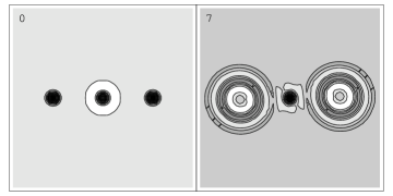
Figure 4: Numerical simulation under initial condition described by Eq. (12). The left figure shows input intensity at $z=0$, a singly charged vortex located at center and two side-locating normal Gaussian dips initially separated by a distance $d=30$. The right figure shows intensity at $z=7$. The simulation parameters are $w=10,\eta=6,d=30$ and the size of each frame is equal to $27\times 27$ unit.

As has been previously indicated7 ; 10 that two separated vortices of the same charge $m=1$ embedded off axis in a finite-size Gaussian beam will rotate around the axis in both the linear and nonlinear cases. The rotation angular speed depends on the propagation distance from the beam waist of the background Gaussian beam and is not a constant. There exits a maximal rotational angle at infinite propagation distance from the beam waist. In this paper we investigate the rotation of vortices embedded in an infinite-size constant background $\eta$. To do so, we consider this following initial amplitude

$$u(x,y,0) ={{1}\over{\eta}}F_{1}(x-d/2,y)e^{i\rm{m}_{1}\varphi(x-d/2,y)}$$ (13)

$$\times F_{2}(x+d/2,y)e^{i\rm{m}_{2}\varphi(x+d/2,y)},$$

which describes two vortices of charge $m_{1}$ and $m_{2}$ initially located at $(d/2,0)$ and $(-d/2,0)$ respectively.

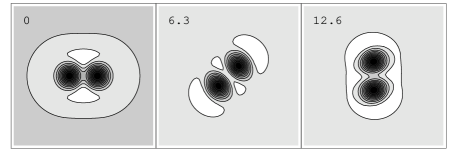
Figure 5: Rotation of two vortices of the same charge $m=1$ initially separated by a distance $d=4$, and $w=10,\eta=6$. The size of each frame is equal to $10\times 10$ unit.

As shown in Figs. (5) the two vortices of the same charge $m=1$ rotate around each other. The rotational angular speed is nearly a constant and there is no limit on the rotational angle of the two vortices. As indicated by table(1), the angular speed does depend on the initial separated distance between vortices.

Table 1: The rotation period $T$ of two vortices of the same charge $m=1$ initially separated by a distance $d$.

d	3	4	5	6	7	8
T	36.1	50.4	73.9	108.8	152.4	200.8
$d^{2}\pi/T$	0.78	0.997	1.06	1.04	1.01	1.001

As has been previously indicated11 ; 12 , in the limit that the interval distances between vortices are much larger than the size of the core of the vortices, the vortices can be viewed as point vortices. For two vortices of the same charge $m=1$ separated by a very large distance $d$, based on the point vortices model it can be deduced that the peripheral speed of each vortex is equal to $1/d$. On the other hand the peripheral speed can be expressed as ${{d}\over{2}}{{2\pi}\over{T}}$, where $T$ is the rotation period. So we have ${{d^{2}\pi}\over{T}}=1$. As indicated by table(1), the point vortices model can give a rather good approximation of the peripheral speed of the vortices for large interval distance.

Annihilation of two vortices of opposite charge $m=1$ and $m=-1$ initially separated by a short enough distance are shown in Fig. (6). It is shown that these two opposite vortices annihilates each other and form a moving trough of the radiated ripples, which qualitatively agrees with the experimental observation by I. V. Basistiy, et. al.7 . It is worth to note that annihilation for two far separated opposite vortices may be hardly possible with absence of other exterior interaction. Figure. (7) may be regarded as a rudimentary proof of this statement. For large interval distance, the point vortices model11 ; 12 predicts the directions of velocities of two vortices of opposite charge $m=-1$ and $m=1$ are the same and perpendicular to the line along these two vortices. So these two far separated vortices will never move close to each other and annihilation cannot occur. From Fig. (7) the co-moving speed of vortices is equal to $11.4/40=0.285$, which is very close to $1/d=1/4=0.25$ predicted by point vortices model.

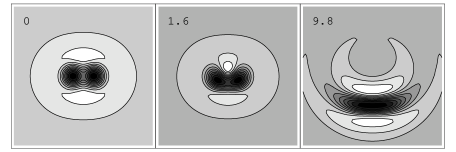
Figure 6: Annihilation of two vortices of opposite charge $m=1$ and $m=-1$ initially separated by a distance $d=3$, and $w=10,\eta=6$. The size of each frame is equal to $10\times 10$ unit.

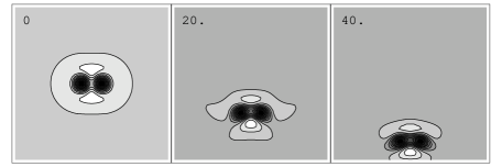
Figure 7: Co-moving but not annihilated two opposite vortices initially separated by a distance $d=4$. The other parameters are the same as Fig. (6) and the size of each frame is equal to $15\times 15$ unit.

Multicharged vortices are topologically unstable2 ; 7 . In reference2 two possible mechanisms that split a multicharged vortex into a set of singly charged vortices are discussed. The first mechanism is due to the fact that multicharged vortices are topologically unstable and separate into a set of singly charged vortices in the presence of a small amount of noise, even in the framework of linear optics2 . The second mechanism is due to propagation effects. Anisotropic initial conditions can result into the splitting of multicharged vortices due to linear diffraction2 . Specifically the reference2 investigated how an elliptically shaped high-charge vortex embedded in a Gaussian beam splits into charge-one vortices. In this paper we consider another anisotropic initial conditons that a singly charged vortex and a charge-two vortex initially separated by a distance co-propagate in a nonlocal media. As shown in Figs. (8) and (9), the charge-two vortex splits into two singly charged vortices with the present of another singly charged vortex. We note the nonlocality of the nonlinear response enhance the anisotropy of the initial conditions. In local nonlinear case, a local region’s perturbed refractive index is solely generated by the vortex located at such a region. So in local nonlinear case two far separated vortices will never affect the perturbed refractive index of the region the other one located at. So the perturbed refractive index of the region the charge-two vortex located at will be isotropic but not anisotropic. The charge-two vortex will not experience the anisotropy due to the present of another far separated vortex in the local nonlinear case and will not split into two singly charged vortices. However in nonlocal nonlinear case, the perturbed refractive index of a region will depend on a distant field. The perturbed refractive index of the region the charge-two vortex located at will be anisotropic due to the present of another far separated vortex. Owing to such anisotropy of the perturbed index, the charge-two vortex splits into two singly charged vortices.

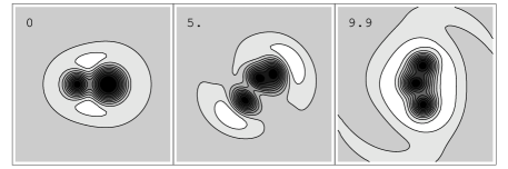
Figure 8: Interaction of two vortices of charge $m=1$ and $m=2$ initially separated by a distance of $d=4$. The other parameters are the same as Fig. (5).

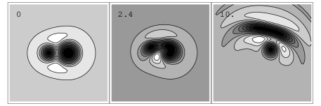
Figure 9: Interaction of two vortices of charge $m=1$ and $m=-2$. The other parameters are the same as Fig. (8).

By the way, in self-focusing nonlocal case, there exist vortex soliton solutions which have a vanishing intensities rather than non-vanishing intensities in self-defocusing case when $r\rightarrow\infty$. Multicharged vortices are topologically unstable too in such self-focusing nonlocal case. And we will predict that the multicharged vortices will also split into singly charged vortics with the present of far separated vortices.

References

- (1) G. A. Swartzlander and C. T. Law, Phys. Rev. Lett, , 2503, (1992).
- (2) A. V. Mamaev, M. Saffman and A. A. Zozulya, Phys. Rev. Lett, , 2108 (1997).
- (3) A. Dreischuh, G. G. Paulus, F. Zacher, F. Grasbon, and H. Walther, Phys. Rev E, , 6111, (1999)
- (4) A. Dreischuh, G. G. Paulus, F. Zacher, F. Grasbon, D. Neshev, and H. Walther, Phys. Rev E, , 7815, (1999)
- (5) C. T. Law and G. A. Swartzlander, Opt. Lett., , 586, (1993)
- (6) H. Sakaguchi and T. Higashiuchi, Phys. Lett A, , 647, (2006)
- (7) I. V. Basistiy, V. Yu. Bazhenov, M. S. Soskin and M. V. Vasnetsov, Opt. Commun., , 422, (1993)
- (8) Igor Aranson and Victor Steinberg, Phys. Rev B, , 75, (1996)
- (9) D. E. Pelinovsky, Y. A. Stepanyants and Y. S. Kivshar, Phys. Rev E, , 5016, (1995)
- (10) B. Luther-Davies, R. Powles, and V. Tikhonenko, Opt. Lett., , 1816, (1994)
- (11) J.C. NEU, Physica D, , 385, (1990)
- (12) F. Lund, Phys. Lett. A, , 245, (1991)
- (13) E. A. Kuznetsov and J. J. Rasmussen, Phys. Rev. E, , 4479, (1995)
- (14) A. W Snyder, L. Poladian, and D. J. Mitchell, Opt. Lett., , 789, (1992)
- (15) I. Velchev, A. Dreischuh, D. Neshev, S. Dinev, Opt. Commun., , 77, (1997)
- (16) S. Baluschev, A. Dreischuh, I. Velchev, S. Dinev and O. Marazov, Phys. Rev. E, , 5517, (1995)
- (17) Mark J. Ablowitz, Ziad H. Musslimani, Opt. Lett, , 2140, (2005).
- (18) V. I. Petviashvili, Fiz. Plazmy , 469 (1976) [Sov. J. Plasma Phys. , 257 (1976)].
- (19) A. A. Zozulya, D. Z. Anderson, A. V. Mamaev and M. Saffman, Phys. Rev. A, , 522, (1998)