Zigzag Persistence

Abstract.

We describe a new methodology for studying persistence of topological features across a family of spaces or point-cloud data sets, called zigzag persistence. Building on classical results about quiver representations, zigzag persistence generalises the highly successful theory of persistent homology and addresses several situations which are not covered by that theory. In this paper we develop theoretical and algorithmic foundations with a view towards applications in topological statistics.

1. Introduction

1.1. Overview

In this paper, we describe a new methodology for studying persistence of topological features across a family of spaces or point-cloud data sets. This theory of zigzag persistence generalises the successful and widely used theory of persistence and persistent homology [Edelsbrunner_L_Z_2002, Zomorodian_Carlsson_2005]. Moreover, zigzag persistence can handle several important situations that are not currently addressed by standard persistence.

The zigzag persistence framework is activated whenever one constructs a zigzag diagram of topological spaces or vector spaces: a sequence of spaces $S_{1},\dots,S_{n}$ where each adjacent pair is connected by a map $S_{i}\to S_{i+1}$ or $S_{i}\leftarrow S_{i+1}$. The novelty of our approach is that the direction of each linking map is arbitrary, in contrast to the usual theory of persistence where all maps point in the same direction.

This paper has three principal objectives:

• To describe several scenarios in applied topology where it is natural to consider zigzag diagrams (Section 1).

• To develop a mathematical theory of persistence for zigzag diagrams (Sections 2 and 3).

• To develop algorithms for computing zigzag persistence (Section 4).

There is one subsidiary objective:

• To introduce the Diamond Principle, a calculational tool analogous in power and effect to the Mayer–Vietoris theorem in classical algebraic topology (Section 5).

This is a theoretical paper rather than an experimental paper, and we devote most of our effort to covering the mathematical foundations adequately. The technical basis for zigzag persistence comes from the theory of graph representations, also known as quiver theory. We are deeply indebted to the practitioners of that theory; what is new here is the emphasis on algorithmics and on applications to topology (particularly Sections 1, 4 and 5).

1.2. Persistence

One of the principal challenges when attempting to apply algebraic topology to statistical data is the fact that traditional invariants — such as the Betti numbers or the fundamental group — are extremely non-robust when it comes to discontinuous changes in the space under consideration. Persistent homology [Edelsbrunner_L_Z_2002, Zomorodian_Carlsson_2005] is the single most powerful existing tool for addressing this problem.

A typical workflow runs as follows [deSilva_Carlsson_2004]. The input is a point cloud, that is, a finite subset of some Euclidean space or more generally a finite metric space. After an initial filtering step (to remove undesirable points or to focus on high-density regions of the data, say), a set of vertices is selected from the data, and a simplicial complex $S$ is built on that vertex set, according to some prearranged rule. In practice, the simplicial complex depends on a coarseness parameter $\epsilon$, and what we have is a nested family $\{S_{\epsilon}\}_{\epsilon\in[0,\infty]}$, which typically ranges from a discrete set of vertices at $S_{0}$ to a complete simplex at $S_{\infty}$.

Persistent homology takes the entire nested family $\{S_{\epsilon}\}$ and produces a barcode or persistence diagram as output. A barcode is a collection of half-open subintervals $[b_{j},d_{j})\subseteq[0,\infty)$, which describes the homology of the family as it varies over $\epsilon$. An interval $[b_{j},d_{j})$ represents a homological feature which is born at time $b_{j}$ and dies at time $d_{j}$. This construction has several excellent properties:

• There is no need to select a particular value of $\epsilon$.

• Features can be evaluated by interval length. Long intervals are expected to indicate essential features of the data, whereas short intervals are likely to be artefacts of noise.

• There exists a fast algorithm to compute the barcode [Zomorodian_Carlsson_2005].

• The barcode is a complete invariant of the homology of the family of complexes [Zomorodian_Carlsson_2005].

• The barcode is provably stable with respect to changes in the input [CohenSteiner_E_H_2007]. In contrast, any individual homology group $H_{k}(S_{\epsilon})$ is highly unstable.

The major limitation of persistence is that it depends crucially on the family $\{S_{\epsilon}\}$ being nested, in the sense that $S_{\epsilon}\subseteq S_{\epsilon^{\prime}}$ whenever $\epsilon\leq\epsilon^{\prime}$. This applies to the current theoretical understanding as well as the algorithms. Zigzag persistence addresses this limitation.

If we discretise the variable $\epsilon$ to a finite set of values, the family of simplicial complexes can be thought of as a diagram of spaces

$$S_{1}\to S_{2}\to\dots\to S_{n}$$

where the arrows represent the inclusion maps. If we apply the $k$-dimensional homology functor $H_{k}(_{;}\mathbb{F})$ with coefficients in a field $\mathbb{F}$, this becomes a diagram of vector spaces

$$V_{1}\to V_{2}\to\dots\to V_{n}$$

and linear maps, where $V_{i}=H_{k}(S_{i};\mathbb{F})$. Such a diagram is called a persistence module. What makes persistence work is that there is a simple algebraic classification of persistence modules up to isomorphism; each possible barcode corresponds to an isomorphism type.

Our goal is to achieve a similar classification for diagrams in which the arrows may point in either direction. This is zigzag persistence, in a nutshell.

1.3. Zigzag diagrams in applied topology

We consider some problems which arise quite naturally in the computational topology of data.

Example 1.1.

Some of the most interesting properties of a point cloud are contained in the estimates of the probability density from which the data are sampled. Deep structure is sometimes revealed after thresholding according to a density estimate (see [Carlsson_I_dS_Z_2008] for an example drawn from visual image analysis). However, the construction of a density estimation function $\rho$ invariably depends on choosing a smoothing parameter: for instance $\rho(x)$ might be defined to be the number of data points within distance $r$ of $x$; here $r$ is the smoothing parameter.

It happens that different choices of smoothing parameter may well reveal different structures in the data; a particularly striking example of this occurs in [Carlsson_I_dS_Z_2008]. Statisticians have invented useful criteria for determining what the ‘appropriate’ value of such a parameter might be for a particular data set; but another point of view would be to analyse all values of the parameter simultaneously, and to study how the topology changes as the parameter varies.

The problem with doing this is that there is no natural relationship between, say, the $25\%$ densest points as measured using two different parameter values. This means that one cannot build an increasing family of spaces using the change in parameters, and so one cannot use persistence to analyze the evolution of the topology. On the other hand, there are natural zigzag sequences which can be used to study this problem. Select a sequence of parameter values $r_{1}<r_{2}<\dots<r_{n}$ and a percentage $p$, and let $X_{r}^{p}$ denote the densest $p\%$ of the point cloud when measured according to parameter value $r$. We can then consider the union sequence

$$X^{p}_{r_{1}}\rightarrow X^{p}_{r_{1}}\cup X^{p}_{r_{2}}\leftarrow X^{p}_{r_{2}}\rightarrow X^{p}_{r_{2}}\cup X^{p}_{r_{3}}\leftarrow X^{p}_{r_{3}}\rightarrow\dots\leftarrow X^{p}_{r_{n}}$$

or the intersection sequence

$$X^{p}_{r_{1}}\leftarrow X^{p}_{r_{1}}\cap X^{p}_{r_{2}}\rightarrow X^{p}_{r_{2}}\leftarrow X^{p}_{r_{2}}\cap X^{p}_{r_{3}}\rightarrow X^{p}_{r_{3}}\leftarrow\dots\rightarrow X^{p}_{r_{n}}.$$

As we see in Section 5.3, there is essentially no difference between the zigzag persistent homology of the union and intersection sequences of a sequence of spaces. Here that assertion needs to be filtered through the process of representing the data subsets $X_{r}^{p}$ as simplicial complexes.

Example 1.2 (Topological bootstrapping).

Suppose we are given a very large point cloud $X$. If it is too large to process directly, we may take a sequence of small samples $X_{1},\dots,X_{n}$ and estimate their topology individually, perhaps obtaining a persistence barcode for each one. How does this reflect the topology of the original sample $X$? On one hand, if most of the barcodes have similar appearance, then one might suppose that $X$ itself will have the same barcode. On the other hand, one needs to be able to distinguish between a single feature detected repeatedly, and multiple features detected randomly but one at a time. If we detect $n$ features in $X_{i}$ on average, are we detecting $n$ features of $X$ with detection probability 1, or $kn$ features with detection probability $1/k$?

Once again, there is a need to correlate features across different instances of the construction. The union sequence comes to the rescue:

$$X_{1}\rightarrow X_{1}\cup X_{2}\leftarrow X_{2}\rightarrow\dots\leftarrow X_{n}$$

In this case, the intersection sequence is not useful at the level of samples, because two sparse samples are unlikely to intersect very much.

The approach in this example is analogous to bootstrapping in statistics, where measurements on a large data set are estimated by making repeated measurements on a set of samples.

Example 1.3.

In computational topology, there exist several techniques for modelling a point cloud data set $X$ by a simplicial complex $S$: the Cech complex, the Vietoris–Rips complex, the alpha complex [Edelsbrunner_Mucke_1994], the witness complex [deSilva_Carlsson_2004], and so on. The witness complex $W(X;L)$, in particular, depends on the choice of a small subset of ‘landmark’ points $L\subset X$ which will serve as the vertex set of $S$. Roughly speaking, a simplex $\sigma$ with vertices in $L$ is included in $W(X;L)$ if there is some $x\in X$ which witnesses it, by being close to all the vertices.

How does the witness complex $W(X;L)$ depend on the choice of landmark set? There is no direct way to compare $W(X;L)$ with $W(X;M)$ for two different choices of landmark sets $L,M$. However, it turns out that one can define a witness bicomplex $W(X;L,M)$ which maps onto each witness complex. The cells are cartesian products $\sigma\times\tau$, where $\sigma,\tau$ have vertices in $L,M$ respectively. A cell $\sigma\times\tau$ is included provided that there exists $x\in X$ which simultaneously witnesses $\sigma$ for $W(X;L)$ and $\tau$ for $W(X;M)$.

Given a sequence $L_{1},\dots,L_{n}$ of landmark subsets, one can then construct the biwitness zigzag:

$$W(X;L_{1})\leftarrow W(X;L_{1},L_{2})\rightarrow W(X;L_{2})\leftarrow\dots\rightarrow W(X;L_{n})$$

Long intervals in the zigzag barcode will then indicate features that persist across the corresponding range of choices of landmark set.

The fundamental requirement is then for a way of assessing, in a zigzag diagram of vector spaces, the degree to which consistent families of elements exist. The point of this paper is that there is such methodology. We will interpret the isomorphism classes of zig-zag diagrams as a special case of the classification problem for quiver representations (see [Derksen_Weyman_2005] for background on this theory). There turns out to be a theorem of Gabriel [Gabriel_1972] which classifies arbitrary diagrams based on Dynkin diagrams, and which shows in particular that the set of isomorphism classes of zigzag diagrams of a given length is parametrised by barcodes — just as persistence modules are. Long intervals in the classification define large families of consistent elements, hence indicate the presence of features stable across samples, landmark sets, or parameter values for a density estimator.

1.4. Organisation of the paper

In Section 2 we describe the theory of decompositions of zigzag modules. These decompositions produce zigzag persistence barcodes analogous to the barcodes of persistent homology. The foundational theorem of Gabriel is stated without proof. In Section 3 we develop the machinery of right-filtrations, which turn out to be the right tool for accessing the decomposition structure of a zigzag module. This is an important section for the reader who wishes to make serious use of zigzag persistence. In Section 4, we present a general-purpose algorithmic framework for calculating zigzag persistence, and we show how this operates in a practical class of examples. The algorithm is based on a proof of Gabriel’s theorem for zigzag modules, included for completeness. Section 5 is devoted to a localisation principle which gives another approach to zigzag barcode calculations. We apply this to prove the Diamond Principle. We use this in turn to compare the zigzag barcodes for two natural zigzag diagrams obtained from a sequence of simplicial complexes.

2. Zigzag Diagrams of Vector Spaces

We work over a field $\mathbb{F}$ which remains fixed throughout this paper. There is no significance to the choice of $\mathbb{F}$. All vector spaces are finite-dimensional.

2.1. Zigzag modules.

Let ${\mathbb{V}}$ denote a sequence of vector spaces and linear maps, of length $n$:

$$V_{1}\stackrel{{\scriptstyle p_{1}}}{{\longleftrightarrow}}V_{2}\stackrel{{\scriptstyle p_{2}}}{{\longleftrightarrow}}\dots\stackrel{{\scriptstyle p_{n-1}}}{{\longleftrightarrow}}V_{n}$$

Each $\stackrel{{\scriptstyle p_{i}}}{{\longleftrightarrow}}$ represents either a forward map $\stackrel{{\scriptstyle f_{i}}}{{\longrightarrow}}$ or a backward map $\stackrel{{\scriptstyle g_{i}}}{{\longleftarrow}}$. The object ${\mathbb{V}}$ is called a zigzag diagram of vector spaces, or simply a zigzag module, over $\mathbb{F}$.

The sequence of symbols $f$ or $g$ is the type of ${\mathbb{V}}$. For instance, a diagram of type $\tau=fgg$ looks like this:

$$V_{1}\stackrel{{\scriptstyle f_{1}}}{{\longrightarrow}}V_{2}\stackrel{{\scriptstyle g_{2}}}{{\longleftarrow}}V_{3}\stackrel{{\scriptstyle g_{3}}}{{\longleftarrow}}V_{4}$$

The length of a type $\tau$ is the length of any diagram of type $\tau$. For example, we say that $fgg$ has length 4. We will usually be considering zigzag modules of a fixed type $\tau$ of length $n$. Such diagrams are called $\tau$-modules, and the class of $\tau$-modules is denoted ${\tau\mathrm{Mod}}$.

Persistence modules (see [Edelsbrunner_L_Z_2002, Zomorodian_Carlsson_2005]) are zigzag modules where all the maps have the forward orientation; in other words, where $\tau=ff\dots f$. As explained in [Zomorodian_Carlsson_2005], persistence modules can be viewed as graded modules over the polynomial ring $\mathbb{F}[t]$. This observation simplifies the analysis of persistence modules quite considerably.

More generally, one can consider graph representations of arbitrary oriented graphs. Zigzag modules constitute the special case where the graph is $A_{n}$ (a path with $n$ vertices and $n-1$ edges) and the orientation is specified by the type $\tau$. In 1972, Gabriel showed that the Dynkin–Coxeter graphs $A_{n}$, $D_{n}$, $E_{6}$, $E_{7}$, $E_{8}$ (arbitrarily oriented) have an especially well-behaved representation theory [Gabriel_1972]. The theory of quivers was launched from this starting block; see [Derksen_Weyman_2005] for a beautiful and transparent introduction. Zigzag persistence is enabled by the good behaviour of $A_{n}$ graph representations.

Remark.

${\tau\mathrm{Mod}}$ has the structure of an abelian category. Given two $\tau$-modules ${\mathbb{V}},{\mathbb{W}}$, a morphism $\alpha:{\mathbb{V}}\to{\mathbb{W}}$ is defined to be a collection of linear maps $\alpha_{i}:V_{i}\to W_{i}$ which satisfy the commutation relations $\alpha_{i+1}f_{i}=h_{i}\alpha_{i}$ or $\alpha_{i}g_{i}=k_{i}\alpha_{i+1}$ for each $i$. (Here the forward and backward maps for ${\mathbb{W}}$ are written $h,k$ respectively.) Morphisms can be composed in the obvious way, and have kernels, images, and cokernels: for instance ${\mathbb{K}}=\operatorname{Ker}(\alpha)$ is the $\tau$-module with spaces $K_{i}=\operatorname{Ker}(V_{i}\to W_{i})$ and maps $f_{i}|_{K_{i}}$ and $g_{i}|_{K_{i+1}}$ defined by restriction. The set of morphisms $\operatorname{Hom}({\mathbb{V}},{\mathbb{W}})$ is naturally a vector space over $\mathbb{F}$, and the endomorphism ring $\operatorname{End}({\mathbb{V}})=\operatorname{Hom}({\mathbb{V}},{\mathbb{V}})$ is a non-commutative $\mathbb{F}$-algebra. We can view $\operatorname{End}({\mathbb{V}})$ as the subalgebra of $\operatorname{End}(V_{1})\times\dots\times\operatorname{End}(V_{n})$ defined by the commutation relations.

2.2. Decompositions of zigzag modules.

We wish to understand zigzag modules by decomposing them into simpler parts. Accordingly, a submodule ${\mathbb{W}}$ of a $\tau$-module ${\mathbb{V}}$ is defined by subspaces $W_{i}\leq V_{i}$ such that $f_{i}(W_{i})\subseteq W_{i+1}$ or $g_{i}(W_{i+1})\subseteq W_{i}$ for all $i$. These conditions guarantee that ${\mathbb{W}}$ is itself a $\tau$-module, with maps given by the restrictions $f_{i}|_{W_{i}}$ or $g_{i}|_{W_{i+1}}$. We write ${\mathbb{W}}\leq{\mathbb{V}}$.

A submodule ${\mathbb{W}}$ is called a summand of ${\mathbb{V}}$ if there exists a submodule ${\mathbb{X}}\leq{\mathbb{V}}$ which is complementary to ${\mathbb{W}}$, in the sense that $V_{i}=W_{i}\oplus X_{i}$ for all $i$. In that case, we say that ${\mathbb{V}}$ is the direct sum of ${\mathbb{W}},{\mathbb{X}}$ and write ${\mathbb{V}}={\mathbb{W}}\oplus{\mathbb{X}}$.

Example 2.1.

As a rule, most submodules are not summands. ${\mathbb{V}}=(\mathbb{F}\stackrel{{\scriptstyle 1}}{{\longrightarrow}}\mathbb{F})$ has the submodule ${\mathbb{W}}=(0\longrightarrow\mathbb{F})$. However, ${\mathbb{W}}$ is not a summand because the only possible complement is $(\mathbb{F}\longrightarrow 0)$, and that is not a submodule of ${\mathbb{V}}$.

Remark.

The direct sum can also be defined as an ‘external’ operation: given $\tau$-modules ${\mathbb{V}},{\mathbb{W}}$ their direct sum ${\mathbb{V}}\oplus{\mathbb{W}}$ is defined to be the $\tau$-module with spaces $V_{i}\oplus W_{i}$ and maps $f_{i}\oplus h_{i}$ or $g_{i}\oplus k_{i}$. (Here the forward and backward maps for ${\mathbb{W}}$ are written $h,k$ respectively.)

A $\tau$-module ${\mathbb{V}}$ is decomposable if it can be written as a direct sum of nonzero submodules, and indecomposable otherwise. Any $\tau$-module ${\mathbb{V}}$ has a Remak decomposition; in other words we can write ${\mathbb{V}}={\mathbb{W}}_{1}\oplus\dots\oplus{\mathbb{W}}_{N}$, where the summands ${\mathbb{W}}_{j}$ are indecomposable. The existence of such a decomposition is proved by induction on the total dimension $\sum_{i}\dim(V_{i})$: if ${\mathbb{V}}$ is decomposable, say ${\mathbb{V}}={\mathbb{W}}\oplus{\mathbb{X}}$, then we may assume inductively that ${\mathbb{W}},{\mathbb{X}}$ have Remak decompositions, and therefore so does ${\mathbb{V}}$. (Base case: if ${\mathbb{V}}$ is indecomposable, then it has a Remak decomposition with one term.)

Remak decompositions themselves are not unique. However, the Krull–Schmidt principle from commutative algebra tells us that the summands in a Remak decomposition are unique up to reordering:

Proposition 2.2.

(Krull–Remak–Schmidt.) Suppose a $\tau$-module ${\mathbb{V}}$ has Remak decompositions

$${\mathbb{V}}={\mathbb{W}}_{1}\oplus\dots\oplus{\mathbb{W}}_{M}\quad\mbox{and}\quad{\mathbb{V}}={\mathbb{X}}_{1}\oplus\dots\oplus{\mathbb{X}}_{N}.$$

Then $M=N$ and there is some permutation $\sigma$ of $\{1,\dots,N\}$ such that ${\mathbb{W}}_{j}\cong{\mathbb{X}}_{\sigma(j)}$ for all $j$.

Proof.

The proof of Theorem 7.5 of Lang [Lang_2005], which is stated for modules in the ordinary sense, can be applied verbatim to our present context; all the required algebraic operations can be carried out within $\operatorname{End}({\mathbb{V}})$. Since our $\tau$-modules have finite total dimension, the ascending and descending chain conditions (acc and dcc) are automatic. ∎

For further context, we refer the reader to an elegant article by Atiyah [Atiyah_1956]; the Krull–Schmidt principle applies in any exact abelian category to objects which satisfy acc and dcc, or a weaker ‘bi-chain condition’ defined by Atiyah. Our category, ${\tau\mathrm{Mod}}$, is included by this formulation.

Thus we can use the multiset $\{{\mathbb{W}}_{j}\}$ as an isomorphism invariant of ${\mathbb{V}}$. For this to be useful, we need to identify the set of indecomposable $\tau$-modules. We now describe a natural collection of indecomposables. For each subinterval $[b,d]$ of the integer sequence $\{1,\dots,n\}$ there is an associated $\tau$-module.

Definition 2.3.

Let $\tau$ be a type of length $n$ and consider integers $1\leq b\leq d\leq n$. The interval $\tau$-module with birth time $b$ and death time $d$ is written ${\mathbb{I}}_{\tau}(b,d)$ and defined with spaces

$$I_{i}=\left\{\begin{array}[]{ll}\mathbb{F}&\mbox{if $b\leq i\leq d$,}\\ 0&\mbox{otherwise;}\end{array}\right.$$

and with identity maps between adjacent copies of $\mathbb{F}$, and zero maps otherwise. When $\tau$ is implicit, we will usually suppress it and simply write ${\mathbb{I}}(b,d)$.

Example.

If $\tau=fgg$ then ${\mathbb{I}}(2,3)$ is the zigzag module

$$0\stackrel{{\scriptstyle 0}}{{\longrightarrow}}\mathbb{F}\stackrel{{\scriptstyle 1}}{{\longleftarrow}}\mathbb{F}\stackrel{{\scriptstyle 0}}{{\longleftarrow}}0.$$

Proposition 2.4.

Interval $\tau$-modules are indecomposable.

Proof.

Suppose ${\mathbb{I}}(b,d)={\mathbb{V}}\oplus{\mathbb{W}}$ and consider two adjacent terms $\mathbb{F}$ connected by an identity map. Since ${\mathbb{V}},{\mathbb{W}}$ are submodules, the dimensions of ${\mathbb{V}}$ and ${\mathbb{W}}$ cannot decrease in the direction of the map; nor, since they are complements, can they increase. Thus $\dim(V_{i})$ and $\dim(W_{i})$ are constant over $b\leq i\leq d$, and in particular one of ${\mathbb{V}},{\mathbb{W}}$ must be zero. ∎

Here is the foundation stone for the theory of zigzag persistence.

Theorem 2.5 (Gabriel).

The indecomposable $\tau$-modules are precisely the intervals ${\mathbb{I}}(b,d)$, where $1\leq b\leq d\leq n=\operatorname{length}(\tau)$. Equivalently, every $\tau$-module can be written as a direct sum of intervals.

Proof.

This is the simplest special case of Gabriel’s theorem, for the graphs $A_{n}$. The original reference (in German) is [Gabriel_1972]. See [Derksen_Weyman_2005] for an accessible overview. ∎

Thus, any $\tau$-module can be described completely up to isomorphism as an unordered list of intervals $[b,d]$, which correspond to its indecomposable summands. This is in exact accordance with the special case of ordinary persistence, where the result is comparatively easy to prove: it is simply the classification of finitely-generated graded modules over the polynomial ring $\mathbb{F}[t]$ (see [Zomorodian_Carlsson_2005]).

The philosophical point is that the decomposition theory of graph representations is somewhat independent of the orientation of the graph edges (see Kac [Kac_1980]). Even in our case this is surprising, because there is no obvious congruence between persistence modules and zigzag modules of an arbitrary type $\tau$. However, if we accept this principle, then the generalisation from ordinary persistence to zigzag persistence is not surprising: interval decomposition for persistence modules implies interval decomposition for zigzag modules.

We will devote much of this paper to constructing a stand-alone proof of Theorem 2.5. This provides technical support towards our two main goals: to provide algorithms for computing the interval summands of a given $\tau$-module; and to make rigorous statements about the output of those algorithms.

2.3. Zigzag persistence.

We now define zigzag persistence and develop some of its elementary properties.

Definition 2.6.

Let ${\mathbb{V}}$ be a zigzag module (of arbitrary type). The zigzag persistence of ${\mathbb{V}}$ is defined to be the multiset

$$\operatorname{Pers}({\mathbb{V}})=\left\{[b_{j},d_{j}]\subseteq\{1,\dots,n\}\mid j=1,\dots,N\right\}$$

of integer intervals derived from a decomposition ${\mathbb{V}}\cong{\mathbb{I}}(b_{1},d_{1})\oplus\cdots\oplus{\mathbb{I}}(b_{N},d_{N})$. The Krull–Schmidt principle asserts that this definition is independent of the decomposition.

Graphically, $\operatorname{Pers}({\mathbb{V}})$ can be represented as a set of lines measured against a single axis with labels $\{1,\dots,n\}$ (the barcode), or as a multiset of points in $\mathbb{R}^{2}$ lying on or above the diagonal in the positive quadrant (the persistence diagram). See Figure 1 for an example presented in each style.

    

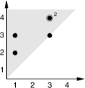
Figure 1. Barcode (left) and persistence diagram (right) representations of the persistence $\{[1,2],[1,3],[3,3],[3,4],[3,4]\}$ of a zigzag module of length 4.

Remark.

In the special case of persistence modules, this agrees with the standard treatment (see [Edelsbrunner_L_Z_2002, Zomorodian_Carlsson_2005]) except in the following particular: the closed integer intervals $[b_{j},d_{j}]\subseteq\{1,\dots,n\}$ are replaced by half-open real intervals $[b_{j},d_{j}+1)\subset\mathbb{R}$ in the standard treatment. This is particularly natural when the indexing parameter is continuous: an interval $[b,d)$ indicates a feature born at time $b$ that survives right up to, but vanishes at, time $d$. Our convention is motivated by the desire to maintain symmetry between the forward and backward directions. We advise the reader to take particular care in handling the different conventions.

The transition from a zigzag module to its interval decomposition presents certain hazards which are not present in the case of persistence modules. We now draw attention to these hazards.

Definition 2.7.

Let ${\mathbb{V}}$ be a zigzag module and let ${\mathbb{V}}[p,q]$ denote the restriction of ${\mathbb{V}}$ to the index set $p\leq i\leq q$. A feature of ${\mathbb{V}}$ over the time interval $[p,q]$ is a summand of ${\mathbb{V}}[p,q]$ isomorphic to ${\mathbb{I}}(p,q)$.

With persistence modules, there are several equivalent ways to recognise the existence of a feature. Here is a sample result.

Proposition 2.8.

Let ${\mathbb{V}}$ be a persistence module of length $n$, and let $1\leq p\leq q\leq n$. The following are equivalent:

1. The composite map $V_{p}\to V_{q}$ is nonzero.

2. There exist nonzero elements $x_{i}\in V_{i}$ for $p\leq i\leq q$, such that $x_{i+1}=f_{i}(x_{i})$ for $p\leq i<q$.

3. There exists a submodule of ${\mathbb{V}}[p,q]$ isomorphic to ${\mathbb{I}}(p,q)$.

4. There exists a summand of ${\mathbb{V}}[p,q]$ isomorphic to ${\mathbb{I}}(p,q)$, i.e. a feature over $[p,q]$.

Proof.

It is easy to verify that (1), (2), (3) are equivalent. For (1) $\Rightarrow$ (2), begin by choosing $x_{p}\in V_{p}$ that maps to a nonzero element in $V_{q}$, and let $x_{i}$ be the image of $x_{p}$ in $V_{i}$. For (2) $\Rightarrow$ (3), define ${\mathbb{I}}$ by $I_{i}=\operatorname{Span}(x_{i})$. For (3) $\Rightarrow$ (1), note that the restriction $I_{p}\to I_{q}$ is nonzero.

Clearly (4) $\Rightarrow$ (3). We now show that (1) $\Rightarrow$ (4). Consider an interval decomposition ${\mathbb{V}}[p,q]={\mathbb{I}}(b_{1},d_{1})\oplus\dots\oplus{\mathbb{I}}(b_{N},d_{N})$. On each summand, the map $I_{p}(b_{j},d_{j})\to I_{q}(b_{j},d_{j})$ is zero unless $b_{j}=p$ and $d_{j}=q$. Thus at least one of the summands is isomorphic to ${\mathbb{I}}(p,q)$. ∎

The intuitions supported by Proposition 2.8 break down in the general case.

Caution 2.9.

Let ${\mathbb{V}}$ be a zigzag module of arbitrary type. Statement (1) has no clear interpretation at this stage (something can be said in terms of the right-filtration functor of Section 3). Consider the following statements:

1. There exist nonzero elements $x_{i}\in V_{i}$ for $p\leq i\leq q$, such that $x_{i+1}=f_{i}(x_{i})$ or $x_{i}=g_{i}(x_{i+1})$ (whichever is applicable) for $p\leq i<q$.

2. There exists a submodule of ${\mathbb{V}}[p,q]$ isomorphic to ${\mathbb{I}}(p,q)$.

3. There exists a summand of ${\mathbb{V}}[p,q]$ isomorphic to ${\mathbb{I}}(p,q)$, i.e. a feature over $[p,q]$.

It is easy to verify that $(2)\Leftrightarrow(3)$ and that (4) implies $(2),(3)$. However, the next two examples demonstrate that $(2),(3)$ do not in general imply (4).

Example 2.10.

Let $\tau=gf$ and consider the $\tau$-module ${\mathbb{V}}$ defined as follows:

$$\begin{diagram}$$

The interval decomposition is ${\mathbb{V}}={\mathbb{I}}(1,2)\oplus{\mathbb{I}}(2,3)$, where the summands are

$$\begin{diagram}$$

and

$$\begin{diagram}$$

respectively. If this example appeared in a statistical topology setting, the feature corresponding to the generator of the $\mathbb{F}$ at $V_{1}$ would be regarded as unrelated to the feature corresponding to the generator of the $\mathbb{F}$ at $V_{3}$.

On the other hand, ${\mathbb{V}}$ does have a submodule (in fact, many submodules) isomorphic to ${\mathbb{I}}(1,3)$. Indeed, let $\Delta=\{(x,x)\mid x\in\mathbb{F}\}$ denote the diagonal subspace of $\mathbb{F}^{2}$. Then

$$\begin{diagram}$$

is a submodule ${\mathbb{W}}\leq{\mathbb{V}}$ isomorphic to ${\mathbb{I}}(1,3)$. The quotient $\tau$-module ${\mathbb{V}}/{\mathbb{W}}$ is isomorphic to ${\mathbb{I}}(2,2)$ but ${\mathbb{W}}$ has no complementary $\tau$-module in ${\mathbb{V}}$. Indeed, that would contradict the Krull–Schmidt theorem. More concretely, any complement of ${\mathbb{W}}$ must be isomorphic to $(0\longleftarrow\mathbb{F}\longrightarrow 0)$, but that would require a 1-dimensional subspace of $\operatorname{Ker}(g_{1})\cap\operatorname{Ker}(f_{2})=0$.

Example 2.11.

We can extend the previous example to arbitrary length. Consider the type $\tau=gf\dots gf=(gf)^{n}$, of length $2n+1$. Let ${\mathbb{V}}$ be the $\tau$-module

$$\mathbb{F}\stackrel{{\scriptstyle\pi_{1}}}{{\longleftarrow}}\mathbb{F}^{2}\stackrel{{\scriptstyle\pi_{2}}}{{\longrightarrow}}\mathbb{F}\stackrel{{\scriptstyle\pi_{1}}}{{\longleftarrow}}\cdots\stackrel{{\scriptstyle\pi_{2}}}{{\longrightarrow}}\mathbb{F}\stackrel{{\scriptstyle\pi_{1}}}{{\longleftarrow}}\mathbb{F}^{2}\stackrel{{\scriptstyle\pi_{2}}}{{\longrightarrow}}\mathbb{F},$$

where $\pi_{1}(x,y)=x$, and $\pi_{2}(x,y)=y$. Then ${\mathbb{V}}$ is isomorphic to a sum of short intervals

$${\mathbb{I}}(1,2)\oplus\left\{{\mathbb{I}}(2,4)\oplus\dots\oplus{\mathbb{I}}(2n-2,2n)\right\}\oplus{\mathbb{I}}(2n,2n+1)$$

but it has a submodule

$$\mathbb{F}\stackrel{{\scriptstyle}}{{\longleftarrow}}\Delta\stackrel{{\scriptstyle}}{{\longrightarrow}}\mathbb{F}\stackrel{{\scriptstyle}}{{\longleftarrow}}\cdots\stackrel{{\scriptstyle}}{{\longrightarrow}}\mathbb{F}\stackrel{{\scriptstyle}}{{\longleftarrow}}\Delta\stackrel{{\scriptstyle}}{{\longrightarrow}}\mathbb{F}$$

isomorphic to the long interval ${\mathbb{I}}(1,2n+1)$.

Moral.

In zigzag persistence it is necessary to respect the distinction between submodules and summands. Features are defined in terms of summands; never submodules.

We have defined features in terms of a chosen subinterval $[p,q]$. Features behave as expected when zooming to a larger or smaller window of observation. The following proposition illustrates what we mean.

Proposition 2.12.

Let ${\mathbb{V}}$ be a zigzag module of length $n$ and let $1\leq p\leq q\leq n$. The following statements are equivalent.

1. There exists a summand of ${\mathbb{V}}[p,q]$ isomorphic to ${\mathbb{I}}(p,q)$, i.e. a feature over $[p,q]$.

2. There exists a summand of ${\mathbb{V}}$ isomorphic to ${\mathbb{I}}(p^{\prime},q^{\prime})$, for some $[p^{\prime},q^{\prime}]\supseteq[p,q]$.

Indeed, there is a bijection between intervals $[p,q]$ in $\operatorname{Pers}({\mathbb{V}}[p,q])$ and intervals $[p^{\prime},q^{\prime}]\supseteq[p,q]$ in $\operatorname{Pers}({\mathbb{V}})$.

Proof.

Consider an interval decomposition ${\mathbb{V}}={\mathbb{I}}(b_{1},d_{1})\oplus\cdots\oplus{\mathbb{I}}(b_{N},d_{N})$. By restriction, this induces an interval decomposition of ${\mathbb{V}}[p,q]$ into intervals ${\mathbb{I}}(b_{j},d_{j})[p,q]$. This induces the claimed bijection, because $[b_{j},d_{j}]$ restricts to $[p,q]$ if and only if $[b_{j},d_{j}]\supseteq[p,q]$. ∎

Operating invisibly in this proof is the Krull–Schmidt principle, which allows us to select the interval decompositions most convenient to us when calculating $\operatorname{Pers}({\mathbb{V}})$ and $\operatorname{Pers}({\mathbb{V}}[p,q])$.

Remark.

Sometimes it is useful to reduce the resolution of $\operatorname{Pers}(V)$. Let $K\subset\{1,\dots,n\}$ be any subset. We define the restriction of $\operatorname{Pers}({\mathbb{V}})$ to $K$ to be the multiset

$$\operatorname{Pers}({\mathbb{V}})|_{K}=\left\{I\cap K\mid I\in\operatorname{Pers}({\mathbb{V}}),\,I\cap K\not=\emptyset\right\}.$$

For instance, Proposition 2.12 amounts to the observation that $\operatorname{Pers}({\mathbb{V}}[p,q])=\operatorname{Pers}({\mathbb{V}})|_{[p,q]}$.

3. From Zigzag Modules to Filtrations

3.1. The right-filtration operator

Our strategy is to understand (and construct) decompositions of a $\tau$-module ${\mathbb{V}}$ by an iterative process, moving from left to right and retaining the necessary information at each stage. The bulk of this information is encoded as a filtration on the rightmost vector space $V_{n}$.

Definition 3.1.

The right-filtration $\mathrm{R}({\mathbb{V}})$ of a $\tau$-module ${\mathbb{V}}$ of length $n$ takes the form

$$\mathrm{R}({\mathbb{V}})=(R_{0},R_{1},\dots,R_{n}),$$

where the $R_{i}$ are subspaces of $V_{n}$ satisfying the inclusion relations

$$0=R_{0}\leq R_{1}\leq\dots\leq R_{n}=V_{n}.$$

$\mathrm{R}({\mathbb{V}})$ is defined recursively as follows.

Base case:

• If ${\mathbb{V}}$ has length 1, then $\mathrm{R}({\mathbb{V}})=(0,V_{1})$.

Recursive step. Suppose we have already defined $\mathrm{R}({\mathbb{V}})=(R_{0},R_{1},\dots,R_{n})$:

• If ${\mathbb{V}}^{+}$ is ${\mathbb{V}}\stackrel{{\scriptstyle f_{n}}}{{\longrightarrow}}V_{n+1}$, then $\mathrm{R}({\mathbb{V}}^{+})=(f_{n}(R_{0}),f_{n}(R_{1}),\dots,f_{n}(R_{n}),V_{n+1})$.

• If ${\mathbb{V}}^{+}$ is ${\mathbb{V}}\stackrel{{\scriptstyle g_{n}}}{{\longleftarrow}}V_{n+1}$, then $\mathrm{R}({\mathbb{V}}^{+})=(0,g_{n}^{-1}(R_{0}),g_{n}^{-1}(R_{1}),\dots,g_{n}^{-1}(R_{n}))$.

To verify that $\mathrm{R}({\mathbb{V}}^{+})$ in the two inductive cases is a filtration of the specified form, note that $R_{i}\leq R_{i+1}$ implies that $f_{n}(R_{i})\leq f_{n}(r_{i+1})$ in the first case, and $g_{n}^{-1}(R_{i})\leq g_{n}^{-1}(R_{i+1})$ in the second case. Moreover $f_{n}(R_{0})=f_{n}(0)=0$, and $g_{n}^{-1}(R_{n})=g_{n}^{-1}(V_{n})=V_{n+1}$.

Example 3.2.

Here are the right-filtrations for the two length-2 types:

$$\mathrm{R}(V_{1}\stackrel{{\scriptstyle f_{1}}}{{\longrightarrow}}V_{2}) = (0,f_{1}(V_{1}),V_{2})$$

$$\mathrm{R}(V_{1}\stackrel{{\scriptstyle g_{1}}}{{\longleftarrow}}V_{2}) = (0,g_{1}^{-1}(0),V_{2})$$

Example 3.3.

Here are the right-filtrations for the four length-3 types:

$$\mathrm{R}(V_{1}\stackrel{{\scriptstyle f_{1}}}{{\longrightarrow}}V_{2}\stackrel{{\scriptstyle f_{2}}}{{\longrightarrow}}V_{3}) = (0,f_{2}f_{1}(V_{1}),f_{2}(V_{2}),V_{3})$$

$$\mathrm{R}(V_{1}\stackrel{{\scriptstyle f_{1}}}{{\longrightarrow}}V_{2}\stackrel{{\scriptstyle g_{2}}}{{\longleftarrow}}V_{3}) = (0,g_{2}^{-1}(0),g_{2}^{-1}f_{1}(V_{1}),V_{3})$$

$$\mathrm{R}(V_{1}\stackrel{{\scriptstyle g_{1}}}{{\longleftarrow}}V_{2}\stackrel{{\scriptstyle f_{2}}}{{\longrightarrow}}V_{3}) = (0,f_{2}g_{1}^{-1}(0),f_{2}(V_{2}),V_{3})$$

$$\mathrm{R}(V_{1}\stackrel{{\scriptstyle g_{1}}}{{\longleftarrow}}V_{2}\stackrel{{\scriptstyle g_{2}}}{{\longleftarrow}}V_{3}) = (0,g_{2}^{-1}(0),g_{2}^{-1}g_{1}^{-1}(0),V_{3})$$

See Figure 2 for a schematic representation.

  

  

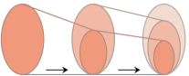
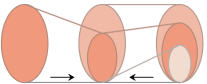
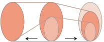
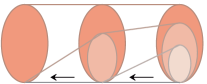
Figure 2. Forward propagation of the right-filtration, illustrated for the four types $ff$, $fg$, $gf$, $gg$ of length 3.

Remark.

In the examples above, it is not difficult to see that $\mathrm{R}({\mathbb{V}})$ comprises all the subspaces of $V_{n}$ that are naturally definable in terms of the maps $p_{i}$.

Each of the $n$ subquotients $R_{i}/R_{i-1}$ carries information dating back to some earliest $V_{j}$ in the sequence of vector spaces.

Example 3.4.

The module $V_{1}\stackrel{{\scriptstyle f_{1}}}{{\longrightarrow}}V_{2}$ has right-filtration $(0,f_{1}(V_{1}),V_{2})$. The first subquotient $f_{1}(V_{1})/0=f_{1}(V_{1})$ corresponds to vectors born at time 1 which survive to time 2. The second subquotient $V_{2}/f_{1}(V_{1})$ corresponds to vectors which appear only at time 2.

Example 3.5.

The module $V_{1}\stackrel{{\scriptstyle g_{1}}}{{\longleftarrow}}V_{2}$ has right-filtration $(0,g_{1}^{-1}(0),V_{2})$. The first subquotient $g_{1}^{-1}(0)$ corresponds to vectors at time 2 which are destroyed when mapping back to time 1. The second subquotient $V_{2}/g_{1}^{-1}(0)$ is isomorphic to $g_{1}(V_{2})$ and records those vectors which survive from time 2 back to time 1.

Definition 3.6.

The birth-time index $\mathrm{b}(\tau)=(b_{1},b_{2},\dots,b_{n})$ is a vector of integers $b_{i}$ which indicate the birth-times associated with the subquotients $R_{i}/R_{i-1}$ of the right-filtration of a $\tau$-module. This is defined recursively as follows.

Base case:

• If $\tau$ is empty (i.e. ${\mathbb{V}}$ has length 1) then $\mathrm{b}(\tau)=(1)$.

Recursive step. Suppose we have already defined $\mathrm{b}(\tau)=(b_{1},b_{2},\dots,b_{n})$:

• If $\tau^{+}$ is $\tau f$ then $\mathrm{b}(\tau^{+})=(b_{1},\dots,b_{n},n+1)$.

• If $\tau^{+}$ is $\tau g$ then $\mathrm{b}(\tau^{+})=(n+1,b_{1},\dots,b_{n})$.

Example 3.7.

At length 2 we have $\mathrm{b}(f)=(1,2)$ whereas $\mathrm{b}(g)=(2,1)$. This is consonant with the discussion in Examples 3.4 and 3.5.

Example 3.8.

Here are the birth-time indices for the types of length 3.

$$\mathrm{b}(ff)=(1,2,3),\qquad\mathrm{b}(fg)=(3,1,2),\qquad\mathrm{b}(gf)=(2,1,3),\qquad\mathrm{b}(gg)=(3,2,1).$$

In summary, the information in a $\tau$-module ${\mathbb{V}}$ which survives to time $n$ is encoded as a filtration $R({\mathbb{V}})$ on $V_{n}$. The ‘age’ of the information at each level of the filtration (i.e. at each subquotient) is recorded in the birth-time index $\mathrm{b}(\tau)$.

For a simplified but precise version of this last claim, we now calculate the right-filtrations of interval $\tau$-modules. In the filtration specified in the following lemma, $J_{i}/J_{i-1}=\mathbb{F}$ is the only non-zero subquotient, corresponding to the birth time $b_{i}$.

Lemma 3.9.

Let $\tau$ be a type of length $n$, with $\mathrm{b}(\tau)=(b_{1},b_{2},\dots,b_{n})$. For each $i=1,2,\dots,n$, we have an isomorphism

$$\mathrm{R}({\mathbb{I}}_{\tau}(b_{i},n))={\mathcal{J}}(i,n),$$

where ${\mathcal{J}}(i,n)=(J_{0},J_{1},\dots,J_{n})$ is the filtration on $\mathbb{F}$ defined by

$$J_{0}=\dots=J_{i-1}=0;\quad J_{i}=\dots=J_{n}=\mathbb{F}.$$

Remark.

We refer to the ${\mathcal{J}}(b,n)$ also as intervals (but now in the category of filtered vector spaces).

Proof.

This is a straightforward calculation by induction on $\tau$. For the base case, $\tau$ is empty and $\mathrm{b}(\tau)=(1)$. Then $\mathrm{R}({\mathbb{I}}(1,1))=(0,\mathbb{F})={\mathcal{J}}(1,1)$ as claimed. Now suppose the result is known for $\tau$, with $\mathrm{b}(\tau)=(b_{1},\dots,b_{n})$. Suppose $\tau^{+}=\tau f$ or $\tau g$. In both cases, write $\mathrm{b}(\tau^{+})=(b_{1}^{+},\dots,b_{n+1}^{+})$.

Case $f$: Suppose that $1\leq i\leq n$; then $b_{i}^{+}=b_{i}$ and therefore

$${\mathbb{I}}_{\tau^{+}}(b_{i}^{+},n+1)=({\mathbb{I}}_{\tau}(b_{i},n)\stackrel{{\scriptstyle 1}}{{\longrightarrow}}\mathbb{F}).$$

Writing $\mathrm{R}({\mathbb{I}}_{\tau}(b_{i},n))={\mathcal{J}}(i,n)=(J_{0},J_{1},\dots,J_{n})$, it follows that

$$\mathrm{R}({\mathbb{I}}_{\tau^{+}}(b_{i}^{+},n+1))=(J_{0},J_{1},\dots,J_{n},\mathbb{F})={\mathcal{J}}(i,n+1).$$

For $i=n+1$, we have $b_{n+1}^{+}=n+1$, and indeed

$$\mathrm{R}({\mathbb{I}}_{\tau^{+}}(n+1,n+1))=\mathrm{R}((\dots)\stackrel{{\scriptstyle 0}}{{\longrightarrow}}\mathbb{F})=(0,\dots,0,\mathbb{F})={\mathcal{J}}(n+1,n+1).$$

Case $g$: Suppose that $2\leq i\leq n+1$; then $b_{i}^{+}=b_{i-1}$ and therefore

$${\mathbb{I}}_{\tau^{+}}(b_{i}^{+},n+1)=({\mathbb{I}}_{\tau}(b_{i-1},n)\stackrel{{\scriptstyle 1}}{{\longleftarrow}}\mathbb{F}).$$

Writing $\mathrm{R}({\mathbb{I}}_{\tau}(b_{i-1},n))={\mathcal{J}}(i-1,n)=(J_{0},J_{1},\dots,J_{n})$, it follows that

$$\mathrm{R}({\mathbb{I}}_{\tau^{+}}(b_{i}^{+},n+1))=(0,J_{0},J_{1},\dots,J_{n})={\mathcal{J}}(i,n+1).$$

For $i=1$, we have $b_{1}^{+}=n+1$ and then

$$\mathrm{R}({\mathbb{I}}_{\tau^{+}}(n+1,n+1))=\mathrm{R}((\dots)\stackrel{{\scriptstyle 0}}{{\longleftarrow}}\mathbb{F})=(0,\mathbb{F},\dots,\mathbb{F})={\mathcal{J}}(1,n+1)$$

as required. ∎

Thus the right-filtration (with the help of the birth-time index) distinguishes the different intervals ${\mathbb{I}}(b,n)$. It gives no information about intervals ${\mathbb{I}}(b,d)$ when $d<n$, since in those cases $I_{n}=0$.

Example 3.10.

Consider $\tau=fgf$, so $\mathrm{b}(\tau)=(b_{1},b_{2},b_{3},b_{4})=(3,1,2,4)$ and in general

$$\mathrm{R}(\,V_{1}\stackrel{{\scriptstyle f_{1}}}{{\longrightarrow}}V_{2}\stackrel{{\scriptstyle g_{2}}}{{\longleftarrow}}V_{3}\stackrel{{\scriptstyle f_{3}}}{{\longrightarrow}}V_{4}\,)=(0,\,f_{3}g_{2}^{-1}(0),\,f_{3}g_{2}^{-1}f_{1}(V_{1}),\,f_{3}(V_{3}),\,V_{4}).$$

In particular,

$$\begin{array}[]{cclccccclcrcc}{\mathbb{I}}(b_{2},4)&=&\mathrm{R}(\,\mathbb{F}&\stackrel{{\scriptstyle 1}}{{\longrightarrow}}&\mathbb{F}&\stackrel{{\scriptstyle 1}}{{\longleftarrow}}&\mathbb{F}&\stackrel{{\scriptstyle 1}}{{\longrightarrow}}&\mathbb{F}\,)&=&(0,\,0,\,\mathbb{F},\,\mathbb{F},\,\mathbb{F})&=&{\mathcal{J}}(2,4)\\ {\mathbb{I}}(b_{3},4)&=&\mathrm{R}(\,0&\stackrel{{\scriptstyle}}{{\longrightarrow}}&\mathbb{F}&\stackrel{{\scriptstyle 1}}{{\longleftarrow}}&\mathbb{F}&\stackrel{{\scriptstyle 1}}{{\longrightarrow}}&\mathbb{F}\,)&=&(0,\,0,\,0,\,\mathbb{F},\,\mathbb{F})&=&{\mathcal{J}}(3,4)\\ {\mathbb{I}}(b_{1},4)&=&\mathrm{R}(\,0&\stackrel{{\scriptstyle}}{{\longrightarrow}}&0&\stackrel{{\scriptstyle}}{{\longleftarrow}}&\mathbb{F}&\stackrel{{\scriptstyle 1}}{{\longrightarrow}}&\mathbb{F}\,)&=&(0,\,\mathbb{F},\,\mathbb{F},\,\mathbb{F},\,\mathbb{F})&=&{\mathcal{J}}(1,4)\\ {\mathbb{I}}(b_{4},4)&=&\mathrm{R}(\,0&\stackrel{{\scriptstyle}}{{\longrightarrow}}&0&\stackrel{{\scriptstyle}}{{\longleftarrow}}&0&\stackrel{{\scriptstyle}}{{\longrightarrow}}&\mathbb{F}\,)&=&(0,\,0,\,0,\,0,\,\mathbb{F})&=&{\mathcal{J}}(4,4)\\ \end{array}$$

which is in accordance with Lemma 3.9.

3.2. Decompositions of filtered vector spaces

We now consider filtered vector spaces in their own right, independently of the connection to zigzag-modules, and develop the theory of Remak decompositions. We will see later that this is the right tool for understanding Remak decompositions of zigzag modules.

A filtered vector space of depth $n$ is a sequence ${\mathcal{R}}=(R_{0},R_{1},\dots,R_{n})$ of vector spaces, where $0=R_{0}\leq R_{1}\leq\dots\leq R_{n}$. The class of such objects is denoted $\operatorname{Filt}_{n}$. The right-filtration $\mathrm{R}({\mathbb{V}})$ of any zigzag module ${\mathbb{V}}$ of length $n$ belongs to this class, as do the intervals ${\mathcal{J}}(i,n)$ defined in Lemma 3.9. Indeed, if ${\mathcal{R}}\in\operatorname{Filt}_{n}$ satisfies $\dim(R_{n})=1$, then ${\mathcal{R}}$ is isomorphic to some ${\mathcal{J}}(i,n)$.

Remark.

$\operatorname{Filt}_{n}$ can be given the structure of a category in a natural way, but it is not quite an abelian category since morphisms do not generally have cokernels.

A filtered vector space ${\mathcal{S}}=(S_{0},S_{1},\dots,S_{n})$ is a subspace of ${\mathcal{R}}$ if $S_{i}\leq R_{i}$ for all $i$. It is appropriate to consider a stronger notion of subspace when dealing with direct-sum decompositions: ${\mathcal{S}}$ is an induced subspace of ${\mathcal{R}}$ if there exists a vector subspace $K\leq R_{n}$ such that $S_{i}=R_{i}\cap K$ for all $i$. In that event, we write ${\mathcal{S}}={\mathcal{R}}\cap K$. Note that $K=R_{n}\cap K=S_{n}$.

We say that ${\mathcal{R}}$ is the direct sum of two subspaces, and write ${\mathcal{R}}={\mathcal{S}}\oplus{\mathcal{T}}$, if $R_{i}=S_{i}\oplus T_{i}$ for all $i$. We claim that ${\mathcal{S}},{\mathcal{T}}$ must be induced subspaces. Note that $S_{n}\cap T_{n}=0$. For each $i$, then, $R_{i}\cap S_{n}$ is a subspace of $R_{i}$ which contains $S_{i}$ and meets $T_{i}\leq T_{n}$ only at 0. It follows that $R_{i}\cap S_{n}=S_{i}$ for all $i$. Thus ${\mathcal{S}}={\mathcal{R}}\cap S_{n}$, and symmetrically ${\mathcal{T}}={\mathcal{R}}\cap T_{n}$.

The general form of a direct-sum decomposition is therefore ${\mathcal{R}}=({\mathcal{R}}\cap K)\oplus({\mathcal{R}}\cap L)$. What are the requirements on $K,L$ to make this a valid decomposition? The direct sum condition implies that $R_{n}=K\oplus L$ as a vector space. Moreover, given a vector space decomposition $R_{n}=K\oplus L$, the further condition

$$R_{i}=\operatorname{Span}\left(R_{i}\cap K,R_{i}\cap L\right)\;\mbox{for all~{}$i$}$$

is necessary and sufficient to guarantee ${\mathcal{R}}=({\mathcal{R}}\cap K)\oplus({\mathcal{R}}\cap L)$.

If ${\mathcal{R}}={\mathcal{S}}\oplus{\mathcal{T}}$, the two subspaces ${\mathcal{S}},{\mathcal{T}}$ are said to be complementary summands. The following fact radically simplifies the decomposition theory of filtered vector spaces.

Proposition 3.11.

Every induced subspace of a filtered vector space has a complementary summand.

Proof.

We are given ${\mathcal{S}}={\mathcal{R}}\cap K$, and seek to construct ${\mathcal{T}}=(T_{0},T_{1},\dots,T_{n})$ such that ${\mathcal{R}}={\mathcal{S}}\oplus{\mathcal{T}}$. We proceed inductively. Since $R_{0}=S_{0}=0$ we take $T_{0}=0$. Now suppose we have chosen $T_{k}$ so that $R_{k}=S_{k}\oplus T_{k}$. In particular, $T_{k}\cap S_{k}=0$. Then

$$T_{k}\cap S_{k+1}\leq T_{k}\cap S_{n}=(T_{k}\cap R_{k})\cap S_{n}=T_{k}\cap(R_{k}\cap S_{n})=T_{k}\cap S_{k}=0.$$

Thus $T_{k}$ and $S_{k+1}$ are independent subspaces of $R_{k+1}$, and so $T_{k}$ can be extended to a complement $T_{k+1}$ of $S_{k+1}$ in $R_{k+1}$. This completes the induction. ∎

Corollary 3.12.

The indecomposables in $\operatorname{Filt}_{n}$ are precisely the intervals ${\mathcal{J}}(i,n)$. Thus, every filtered vector space can be decomposed as a finite direct sum of intervals.

Proof.

By Proposition 3.11, ${\mathcal{R}}$ has nontrivial summands if and only if $R_{n}$ has nontrivial vector subspaces; this happens exactly when $\dim(R_{n})>1$. ∎

The dimension of ${\mathcal{R}}\in\operatorname{Filt}_{n}$ is defined to be the vector of integers

$$\dim({\mathcal{R}})=(c_{1},c_{2},\dots,c_{n}),$$

where $c_{i}=\dim(R_{i}/R_{i-1})$ are the dimensions of the successive subquotients of the filtration.

Proposition 3.13.

Let ${\mathcal{R}}$ be a filtered vector space of depth $n$, with $\dim({\mathcal{R}})=(c_{1},c_{2},\dots,c_{n})$. For any decomposition of ${\mathcal{R}}$ into intervals, the multiplicity of ${\mathcal{J}}(i,n)$ is $c_{i}$. Thus:

$${\mathcal{R}}\cong\bigoplus_{1\leq i\leq n}c_{i}\,{\mathcal{J}}(i,n).$$

Proof.

Let $m_{i}$ be the multiplicity of ${\mathcal{J}}(i,n)$. Then, for all $k$,

$$\dim(R_{k})=m_{1}+m_{2}+\dots+m_{k}$$

by considering the contribution of each summand, whereas

$$\dim(R_{k})=c_{1}+c_{2}+\dots+c_{k}$$

by considering the contribution of each subquotient $R_{i}/R_{i-1}$. This is possible only if $m_{i}=c_{i}$ for all $i$. ∎

This concludes our tour of the decomposition theory for filtered vector spaces. Now we must leverage this to achieve a decomposition theory for $\tau$-modules. In one direction, the relationship is straightforward:

Proposition 3.14.

The right-filtration operation respects direct sums, in the sense that

$$\mathrm{R}({\mathbb{V}}_{1}\oplus\dots\oplus{\mathbb{V}}_{N})=\mathrm{R}({\mathbb{V}}_{1})\oplus\dots\oplus\mathrm{R}({\mathbb{V}}_{N})$$

for $\tau$-modules ${\mathbb{V}}_{1},\dots,{\mathbb{V}}_{N}$.

Proof.

This is proved by induction on $\tau$, following the recursive structure of Definition 3.1 and using the standard facts

$$(f_{1}\oplus\dots\oplus f_{N})(R_{1}\oplus\dots\oplus R_{N})=f_{1}(R_{1})\oplus\dots\oplus f_{N}(R_{N})$$

and

$$(g_{1}\oplus\dots\oplus g_{N})^{-1}(R_{1}\oplus\dots\oplus R_{N})=g_{1}^{-1}(R_{1})\oplus\dots\oplus g_{N}^{-1}(R_{N})$$

from linear algebra. (For simplicity we are suppressing various indices here.) ∎

However, what we need is a converse to Proposition 3.14: if the filtered vector space ${\mathcal{R}}=\mathrm{R}({\mathbb{V}})$ can be split as a direct sum ${\mathcal{R}}={\mathcal{R}}_{1}\oplus\dots\oplus{\mathcal{R}}_{N}$, we would like to infer a corresponding splitting ${\mathbb{V}}={\mathbb{V}}_{1}\oplus\dots\oplus{\mathbb{V}}_{N}$ of $\tau$-modules. In the following two sections we establish such a principle for a particular class: the ‘streamlined’ $\tau$-modules.

3.3. Streamlined modules

We introduce a special class of $\tau$-module for which the right-filtration functor preserves all structural information.

Definition 3.15.

A $\tau$-module ${\mathbb{V}}$ is (right-)streamlined if each $\stackrel{{\scriptstyle f_{i}}}{{\longrightarrow}}$ is injective and each $\stackrel{{\scriptstyle g_{i}}}{{\longleftarrow}}$ is surjective.

Similarly, we may say that a $\tau$-module ${\mathbb{V}}$ is left-streamlined if each $\stackrel{{\scriptstyle f_{i}}}{{\longrightarrow}}$ is surjective and each $\stackrel{{\scriptstyle g_{i}}}{{\longleftarrow}}$ is injective. We will not need to consider left-streamlined modules until Section 5. By default, ‘streamlined’ will be taken to mean ‘right-streamlined’.

Example 3.16.

Intervals ${\mathbb{I}}(b,n)$ are streamlined (but not ${\mathbb{I}}(b,d)$ for $d<n$). Conversely, a streamlined $\tau$-module ${\mathbb{V}}$ with $\dim(V_{n})=1$ is necessarily isomorphic to some ${\mathbb{I}}(b,n)$. Indeed, $\dim(V_{i})$ is a non-decreasing sequence and therefore comprises some $b-1$ zeros (where $1\leq b\leq n$) followed by $n-b+1$ ones. The maps between the one-dimensional terms are injective or surjective, and therefore isomorphisms.

Proposition 3.17.

A direct sum ${\mathbb{V}}={\mathbb{V}}_{1}\oplus\dots\oplus{\mathbb{V}}_{N}$ of $\tau$-modules is streamlined if and only if each summand is streamlined.

Proof.

Each $\stackrel{{\scriptstyle f}}{{\longrightarrow}}$ in ${\mathbb{V}}$ decomposes as $f=f_{1}\oplus\dots\oplus f_{N}$ and is injective if and only if each $f_{j}$ is injective. Each $\stackrel{{\scriptstyle g}}{{\longleftarrow}}$ in ${\mathbb{V}}$ decomposes as $g=g_{1}\oplus\dots\oplus g_{N}$ and is surjective if and only if each $g_{j}$ is surjective. ∎

The proof of the following lemma appears at the end of this section.

Lemma 3.18 (Decomposition Lemma).

Let ${\mathbb{V}}$ be a streamlined $\tau$-module and let ${\mathcal{R}}=\mathrm{R}({\mathbb{V}})$. For any decomposition ${\mathcal{R}}={\mathcal{S}}_{1}\oplus\dots\oplus{\mathcal{S}}_{N}$, there exists a unique decomposition ${\mathbb{V}}={\mathbb{W}}_{1}\oplus\dots\oplus{\mathbb{W}}_{N}$ such that ${\mathcal{S}}_{i}=\mathrm{R}({\mathbb{W}}_{j})$ for all $j$.

Theorem 3.19 (Interval decomposition for streamlined modules).

Let ${\mathbb{V}}$ be a streamlined $\tau$-module of length $n$, and write $\dim(\mathrm{R}({\mathbb{V}}))=(c_{1},c_{2},\dots,c_{n})$ and $\mathrm{b}(\tau)=(b_{1},b_{2},\dots,b_{n})$. Then there is an isomorphism of $\tau$-modules

$${\mathbb{V}}\cong\bigoplus_{1\leq i\leq n}c_{i}\,{\mathbb{I}}(b_{i},n).$$

Proof.

Let ${\mathcal{R}}=\mathrm{R}({\mathbb{V}})$. By Proposition 3.13, there is a decomposition ${\mathcal{R}}={\mathcal{J}}_{1}\oplus\dots\oplus{\mathcal{J}}_{N}$, where the ${\mathcal{J}}_{j}$ are a collection of $N=c_{1}+\dots+c_{n}$ intervals with ${\mathcal{J}}(i,n)$ occuring with multiplicity $c_{i}$. Lemma 3.18 produces a decomposition ${\mathbb{V}}={\mathbb{I}}_{1}\oplus\dots\oplus{\mathbb{I}}_{N}$, with $\mathrm{R}({\mathbb{I}}_{j})={\mathcal{J}}_{j}$ for all $j$. Each ${\mathbb{I}}_{j}$ is streamlined (Proposition 3.17) with maximum dimension $\dim((I_{j})_{n})=1$, and is therefore isomorphic to some ${\mathbb{I}}(b,n)$ (Example 3.16). By Lemma 3.9, we must have ${\mathbb{I}}_{j}={\mathbb{I}}(b_{i},n)$ whenever ${\mathcal{J}}_{j}={\mathcal{J}}(i,n)$. It follows that the ${\mathbb{I}}_{j}$ are a collection of $N=c_{1}+\dots+c_{n}$ intervals with ${\mathbb{I}}(b_{i},n)$ occuring with multiplicity $c_{i}$. ∎

We complete this chapter with a proof of the Decomposition Lemma.

Proof of Lemma 3.18.

We may assume that $N=2$, since the general case follows by iteration. Accordingly, suppose that ${\mathcal{R}}=\mathrm{R}({\mathbb{V}})$ can be written in the form ${\mathcal{R}}={\mathcal{S}}\oplus{\mathcal{T}}$; we must show that there is a corresponding decomposition ${\mathbb{V}}={\mathbb{W}}\oplus{\mathbb{X}}$. We will argue by induction on $n=\operatorname{\rm length}(\tau)$.

The first step is to determine the splitting $V_{n}=W_{n}\oplus X_{n}$. In fact, the stipulation that ${\mathcal{S}}=\mathrm{R}({\mathbb{W}})$ and ${\mathcal{T}}=\mathrm{R}({\mathbb{X}})$ forces $W_{n}=S_{n}$ and $X_{n}=T_{n}$. If $n=1$, then we are done. Otherwise, let $\hat{\mathbb{V}}$ denote the truncation of ${\mathbb{V}}$ to the indices $\{1,\dots,n-1\}$ and let $\hat{\mathcal{R}}=\mathrm{R}(\hat{\mathbb{V}})$. We will shortly establish that ${\mathcal{R}}={\mathcal{S}}\oplus{\mathcal{T}}$ induces a unique compatible decomposition $\hat{\mathcal{R}}=\hat{\mathcal{S}}\oplus\hat{\mathcal{T}}$. The inductive hypothesis will then provide $\hat{\mathbb{V}}=\hat{\mathbb{W}}\oplus\hat{\mathbb{X}}$, which combines with $V_{n}=W_{n}\oplus X_{n}$ to produce the desired decomposition ${\mathbb{V}}={\mathbb{W}}\oplus{\mathbb{X}}$. That will complete the proof.

Write ${\mathcal{R}}=(R_{0},R_{1},\dots,R_{n})$. There are two cases.

Case $\stackrel{{\scriptstyle f_{n-1}}}{{\longrightarrow}}$, injective. We can identify $V_{n-1}$ with the subspace $f_{n-1}(V_{n-1})=R_{n-1}$ of $V_{n}$. Thereupon we have

$$\hat{\mathcal{R}}=(R_{0},R_{1},\dots,R_{n-1}).$$

The unique splitting of $V_{n-1}$ compatible with $V_{n}=W_{n}\oplus X_{n}$ is

$$V_{n-1}=(R_{n-1}\cap W_{n})\oplus(R_{n-1}\cap X_{n})=S_{n-1}\oplus T_{n-1}.$$

We must now verify that the induced subspaces $\hat{\mathcal{S}}=\hat{\mathcal{R}}\cap S_{n-1}$ and $\hat{\mathcal{T}}=\hat{\mathcal{R}}\cap T_{n-1}$ give a valid decomposition $\hat{\mathcal{R}}=\hat{\mathcal{S}}\oplus\hat{\mathcal{T}}$ of filtered vector spaces. This follows because $\hat{S}_{i}=R_{i}\cap S_{n-1}=R_{i}\cap S_{n}=S_{i}$ and similarly $\hat{T}_{i}=T_{i}$, for all $i<n$; so $R_{i}=S_{i}\oplus T_{i}=\hat{S}_{i}\oplus\hat{T}_{i}$ as required.

Case $\stackrel{{\scriptstyle g_{n_{1}}}}{{\longleftarrow}}$, surjective. Here we identify $V_{n-1}$ as the quotient $V_{n}/\ker(g_{n-1})=R_{n}/R_{1}$. Under this identification,

$$\hat{\mathcal{R}}=(R_{1}/R_{1},R_{2}/R_{1},\dots,R_{n}/R_{1}).$$

In splitting $V_{n-1}=W_{n-1}\oplus X_{n-1}$ we are compelled to take

$$W_{n-1}=g_{n-1}(W_{n})=S_{n}/S_{1},\qquad X_{n-1}=g_{n-1}(X_{n})=T_{n}/T_{1},$$

which induce

$$\hat{S}_{i}=g_{n-1}(S_{i+1})=S_{i+1}/S_{1},\qquad\hat{T}_{i}=g_{n-1}(T_{i+1})=T_{i+1}/T_{1},$$

for the purported splitting $\hat{\mathcal{R}}=\hat{\mathcal{S}}\oplus\hat{\mathcal{T}}$. To confirm that this is a genuine decomposition, we note from linear algebra that the twin facts

$$R_{i+1}=S_{i+1}\oplus T_{i+1},\qquad R_{1}=S_{1}\oplus T_{1}=(S_{i+1}\cap R_{1})\oplus(T_{i+1}\cap R_{1})$$

imply that

$$R_{i+1}/R_{1}=(S_{i+1}/S_{1})\oplus(T_{i+1}/T_{1})$$

as required. ∎

Remark.

There is a high-level proof of Lemma 3.18 which in some sense is the natural explanation for the result. We outline this proof now. The first observation is that the transformation ${\mathbb{V}}\to\mathrm{R}({\mathbb{V}})$ is a functor from ${\tau\mathrm{Mod}}$ to $\operatorname{Filt}_{n}$: a morphism $\alpha:{\mathbb{V}}\to{\mathbb{W}}$ induces a morphism $\mathrm{R}(\alpha):\mathrm{R}({\mathbb{V}})\to\mathrm{R}({\mathbb{W}})$. Indeed, $\mathrm{R}(\alpha)$ is defined to be $\alpha_{n}:V_{n}\to W_{n}$; one must check that this respects the filtrations on $V_{n}$ and $W_{n}$. Being a functor, $\mathrm{R}$ defines a ring homomorphism $\operatorname{End}({\mathbb{V}})\to\operatorname{End}(\mathrm{R}({\mathbb{V}}))$. The second key fact is that this homomorphism is an isomorphism if ${\mathbb{V}}$ is streamlined (in general it is surjective). It is well known that direct-sum decompositions of a module can be extracted from the structure of its endomorphism ring: direct summands correspond to idempotent elements of the ring. It follows that ${\mathbb{V}}$ and $\mathrm{R}({\mathbb{V}})$ have the same decomposition structure.

4. The Interval Decomposition Algorithm

Here we describe the algorithm for determining the indecomposable factors of a $\tau$-module. We give three versions of the ‘algorithm’.

The first version, in Section 4.1, is not an algorithm but a proof that every $\tau$-module decomposes as a sum of interval modules (Theorem 2.5). Moreover, the structure of the proof makes it clear how to compute the interval decomposition (Theorem 4.1). The algorithms in the subsequent sections build on this.

In Section 4.2 we describe an abstract form of the decomposition algorithm, using the language of vector spaces and linear maps. No consideration is given to how the spaces and maps are described and manipulated in practice.

In Section 4.3 we suppose that the maps $f_{i},g_{i}$ are presented concretely as matrices $M_{i},N_{i}$ with respect to a choice of bases for the vector spaces $V_{i}$. We describe an algorithm which takes these matrices as input and returns the interval decomposition.

4.1. The interval decomposition theorem

Our present goal is to give a somewhat constructive proof of Theorem 2.5, which asserts that any $\tau$-module ${\mathbb{V}}$ is isomorphic to a direct sum of intervals ${\mathbb{I}}(b,d)$. We prove a stronger, more precise result, which explicitly determines the multiplicity of each interval within ${\mathbb{V}}$.

Some notation will help with the theorem statement. If

$${\mathbb{V}}=(V_{1}\stackrel{{\scriptstyle p_{1}}}{{\longleftrightarrow}}\dots\stackrel{{\scriptstyle p_{n-1}}}{{\longleftrightarrow}}V_{n})$$

then let

$${\mathbb{V}}[k]=(V_{1}\stackrel{{\scriptstyle p_{1}}}{{\longleftrightarrow}}\dots\stackrel{{\scriptstyle p_{k-1}}}{{\longleftrightarrow}}V_{k})$$

denote the truncation of ${\mathbb{V}}$ to length $k$, and let $\tau[k]$ denote its type (which is a truncation of $\tau$).

Theorem 4.1 (Interval decomposition).

Let ${\mathbb{V}}$ be a $\tau$-module. For $1\leq k\leq n$, define

$$(b_{1}^{k},b_{2}^{k},\dots,b_{k}^{k})=\mathrm{b}(\tau[k]).$$

Writing ${\mathcal{R}}_{k}=\mathrm{R}({\mathbb{V}}[k])$, define

$$(c_{1}^{k},c_{2}^{k},\dots,c_{k}^{k})=\left\{\begin{array}[]{l}\dim({\mathcal{R}}_{k}\cap\operatorname{Ker}(f_{k}))\\ \dim({\mathcal{R}}_{k})-\dim({\mathcal{R}}_{k}\cap\operatorname{Im}(g_{k}))\end{array}\right.$$

(whichever is applicable) when $k\neq n$, and

$$(c_{1}^{n},c_{2}^{n},\dots,c_{n}^{n})=\dim({\mathcal{R}}_{n}).$$

Then

$${\mathbb{V}}\cong\bigoplus_{1\leq i\leq k\leq n}c_{i}^{k}\,{\mathbb{I}}(b_{i}^{k},k).$$

Addendum 4.2.

In the situation of Theorem 4.1, write

$$(r^{k}_{1},\dots,r^{k}_{k})=\dim({\mathcal{R}}_{k})$$

for $k=1,\dots,n$, and conventionally define $r^{n+1}_{i}=0$ for all $i$. Then

$$c^{k}_{i}=\left\{\begin{array}[]{ll}r^{k}_{i}-r^{k+1}_{i}&\qquad\mbox{\rm case~{}$\stackrel{{\scriptstyle f_{k}}}{{\longrightarrow}}$}\\ r^{k}_{i}-r^{k+1}_{i+1}&\qquad\mbox{\rm case~{}$\stackrel{{\scriptstyle g_{k}}}{{\longleftarrow}}$}\end{array}\right.$$

for $1\leq i\leq k\leq n$.

The decomposition strategy begins with the following lemma. The idea is to proceed from left to right along the complex, removing streamlined summands at each step. Having done this, the Remak decompositions of those summands can be determined by counting dimensions, as prescribed in Theorem 3.19.

Lemma 4.3.

Let ${\mathbb{V}}=V_{1}\stackrel{{\scriptstyle p_{1}}}{{\longleftrightarrow}}\dots\stackrel{{\scriptstyle p_{n-1}}}{{\longleftrightarrow}}V_{n}$ be an irreducible $\tau$-module of length $n$. Then there exists a direct-sum decomposition

$${\mathbb{V}}={\mathbb{V}}^{1}\oplus{\mathbb{V}}^{2}\oplus\dots\oplus{\mathbb{V}}^{n}$$

where each ${\mathbb{V}}^{k}$ is supported over the indices $\{1,2,\dots,k\}$ and is right-streamlined over that range.

The following picture illustrates the decomposition.

$${\mathbb{V}}=\left\{\begin{array}[]{ccccccccccc}{\mathbb{V}}^{1}&=&V^{1}_{1}\\ \oplus\\ {\mathbb{V}}^{2}&=&V^{2}_{1}&\stackrel{{\scriptstyle p_{1}}}{{\longleftrightarrow}}&V^{2}_{2}\\ \oplus\\ {\mathbb{V}}^{3}&=&V^{3}_{1}&\stackrel{{\scriptstyle p_{1}}}{{\longleftrightarrow}}&V^{3}_{2}&\stackrel{{\scriptstyle p_{2}}}{{\longleftrightarrow}}&V^{3}_{3}\\ \oplus\\ \vdots\\ \oplus\\ {\mathbb{V}}^{n}&=&V^{n}_{1}&\stackrel{{\scriptstyle p_{1}}}{{\longleftrightarrow}}&V^{n}_{2}&\stackrel{{\scriptstyle p_{2}}}{{\longleftrightarrow}}&V^{n}_{3}&\stackrel{{\scriptstyle p_{3}}}{{\longleftrightarrow}}&\cdots&\stackrel{{\scriptstyle p_{n-1}}}{{\longleftrightarrow}}&V^{n}_{n}\end{array}\right.$$

Each row (i.e. summand) is right-streamlined, and therefore amenable to analysis via the right-filtration functor.

Proof.

We proceed by induction on the length of ${\mathbb{V}}$. The inductive statement is that

$${\mathbb{V}}[k]={\mathbb{V}}^{1}\oplus\dots\oplus{\mathbb{V}}^{k-1}\oplus{\mathbb{W}}^{k}$$

where the ${\mathbb{V}}^{i}$ are as in the theorem statement, and ${\mathbb{W}}^{k}$ is itself right-streamlined.

For the base case $k=1$, there is nothing to prove: take ${\mathbb{W}}^{1}={\mathbb{V}}[1]$. Now suppose the inductive statement is established for $k$, and consider ${\mathbb{V}}[k+1]$. This can be written

$$V[k+1] = ({\mathbb{V}}^{1}\oplus\dots\oplus{\mathbb{V}}^{k-1}\oplus{\mathbb{W}}^{k})\stackrel{{\scriptstyle p_{k}}}{{\longleftrightarrow}}V_{k+1}$$

$$= {\mathbb{V}}^{1}\oplus\dots\oplus{\mathbb{V}}^{k-1}\oplus({\mathbb{W}}^{k}\stackrel{{\scriptstyle p_{k}}}{{\longleftrightarrow}}V_{k+1})$$

where the rebracketing is permissible because all of the ${\mathbb{V}}^{i}$ terms terminate before time $k$, and therefore do not interact with $\stackrel{{\scriptstyle p_{k}}}{{\longleftrightarrow}}$. The goal now is to rewrite $({\mathbb{W}}^{k}\stackrel{{\scriptstyle p_{k}}}{{\longleftrightarrow}}V_{k+1})$ as ${\mathbb{V}}^{k}\oplus{\mathbb{W}}^{k+1}$, where ${\mathbb{V}}^{k}$ terminates at time $k$ and both ${\mathbb{V}}^{k}$ and ${\mathbb{W}}^{k+1}$ are right-streamlined. The rightmost term of ${\mathbb{W}}^{k}$ is $V_{k}$, so $\mathrm{R}({\mathbb{W}}^{k})$ is a filtration on $V_{k}$.

Case $f$: ${\mathbb{W}}^{k}\stackrel{{\scriptstyle f_{k}}}{{\longrightarrow}}V_{k+1}$. In other words $f_{k}:V_{k}\to V_{k+1}$. Let ${\mathcal{S}}=\mathrm{R}({\mathbb{W}}^{k})\cap\operatorname{Ker}(f_{k})$. Proposition 3.11 implies that ${\mathcal{S}}$ has a complement in $\mathrm{R}({\mathbb{W}}^{k})$; say $\mathrm{R}({\mathbb{W}}^{k})={\mathcal{S}}\oplus{\mathcal{T}}$. This corresponds (Lemma 3.18) to a direct sum decomposition ${\mathbb{W}}^{k}={\mathbb{V}}^{k}\oplus\hat{\mathbb{W}}^{k}$, where both summands are streamlined (Proposition 3.17). This defines ${\mathbb{V}}^{k}$, and we set ${\mathbb{W}}^{k+1}=(\hat{\mathbb{W}}^{k}\stackrel{{\scriptstyle f_{k}}}{{\longrightarrow}}V_{k+1})$. To check that this works, note that $f_{k}$ is zero on $({\mathbb{V}}^{k})_{k}=\operatorname{Ker}(f_{k})$ and is injective on the complementary subspace $(\hat{\mathbb{W}}^{k})_{k}$. Thus ${\mathbb{V}}^{k}$ is a summand of ${\mathbb{V}}[k+1]$ terminating at time $k$, and ${\mathbb{W}}^{k+1}$ is streamlined.

Case $g$: ${\mathbb{W}}^{k}\stackrel{{\scriptstyle g_{k}}}{{\longleftarrow}}V_{k+1}$. In other words $g_{k}:V_{k+1}\to V_{k}$. Let ${\mathcal{S}}=\mathrm{R}({\mathbb{W}}^{k})\cap\operatorname{Im}(g_{k})$. Proposition 3.11 implies that ${\mathcal{S}}$ has a complement in $\mathrm{R}({\mathbb{W}}^{k})$; say $\mathrm{R}({\mathbb{W}}^{k})={\mathcal{S}}\oplus{\mathcal{T}}$. This corresponds (Lemma 3.18) to a direct sum decomposition ${\mathbb{W}}^{k}=\hat{\mathbb{W}}^{k}\oplus{\mathbb{V}}^{k}$, where both summands are streamlined (Proposition 3.17). This defines ${\mathbb{V}}^{k}$, and we set ${\mathbb{W}}^{k+1}=(\hat{\mathbb{W}}^{k}\stackrel{{\scriptstyle g_{k}}}{{\longleftarrow}}V_{k+1})$. To check that this works, note that $g_{k}$ is surjective onto $(\hat{\mathbb{W}}^{k})_{k}=\operatorname{Im}(g_{k})$ and misses the complementary subspace $({\mathbb{V}}^{k})_{k}$. Thus ${\mathbb{V}}^{k}$ is a summand of ${\mathbb{V}}[k+1]$ terminating at time $k$, and ${\mathbb{W}}^{k+1}$ is streamlined.

This establishes the inductive step, so eventually

$${\mathbb{V}}={\mathbb{V}}[n]={\mathbb{V}}^{1}\oplus\dots\oplus{\mathbb{V}}^{n-1}\oplus{\mathbb{W}}^{n}$$

and we set ${\mathbb{V}}^{n}={\mathbb{W}}^{n}$ to finish the proof. ∎

Proof of Theorem 4.1.

Write ${\mathbb{V}}={\mathbb{V}}^{1}\oplus\dots\oplus{\mathbb{V}}^{n}$ according to Lemma 4.3. We now calculate the decomposition of each ${\mathbb{V}}^{k}$ into intervals ${\mathbb{I}}(b,k)$. Note that

$${\mathbb{V}}[k]={\mathbb{V}}^{k}\oplus{\mathbb{V}}^{k+1}[k]\oplus\dots\oplus{\mathbb{V}}^{n}[k].$$

We can write ${\mathbb{W}}^{k}={\mathbb{V}}^{k+1}\oplus\dots\oplus{\mathbb{V}}^{n}$, so then

$${\mathcal{R}}_{k}=\mathrm{R}({\mathbb{V}}^{k}\oplus{\mathbb{W}}^{k}[k])=\mathrm{R}({\mathbb{V}}^{k})\oplus\mathrm{R}({\mathbb{W}}^{k}[k])$$

(using Proposition 3.14). This is a filtration on $V^{k}_{k}\oplus W^{k}_{k}$.

Suppose $k<n$. We note that ${\mathbb{W}}^{k}$ is streamlined up to time $k+1$, whereas ${\mathbb{V}}^{k}$ is zero at time $k+1$. The next map in the sequence is

$$V^{k}_{k}\oplus W^{k}_{k}\stackrel{{\scriptstyle f_{k}}}{{\longrightarrow}}W^{k}_{k+1}\qquad\mbox{or}\qquad V^{k}_{k}\oplus W^{k}_{k}\stackrel{{\scriptstyle g_{k}}}{{\longleftarrow}}W^{k}_{k+1}.$$

In the first case, it follows that $V^{k}_{k}=\operatorname{Ker}(f_{k})$ and therefore $\mathrm{R}({\mathbb{V}}^{k})={\mathcal{R}}_{k}\cap\operatorname{Ker}(f_{k})$. In the second case, $V^{k}_{k}$ is a complement to $\operatorname{Im}(g_{k})$ in $V_{k}$, so ${\mathcal{R}}_{k}=\mathrm{R}({\mathbb{V}}^{k})\oplus({\mathcal{R}}_{k}\cap\operatorname{Im}(g_{k}))$. Thus

$$\dim(\mathrm{R}({\mathbb{V}}^{k}))=\left\{\begin{array}[]{l}\dim({\mathcal{R}}_{k}\cap\operatorname{Ker}(f_{k}))\\ \dim({\mathcal{R}}_{k})-\dim({\mathcal{R}}_{k}\cap\operatorname{Im}(g_{k}))\end{array}\right\}=(c^{k}_{1},\dots,c^{k}_{k})$$

(whichever middle term is applicable). When $k=n$, moreover, we have

$$\dim(\mathrm{R}({\mathbb{V}}^{n}))=\dim({\mathcal{R}}_{n})=(c^{n}_{1},\dots,c^{n}_{n}).$$

Thus, at last,

$${\mathbb{V}}=\bigoplus_{1\leq k\leq n}{\mathbb{V}}^{k}\cong\bigoplus_{1\leq k\leq n}\left\{\bigoplus_{1\leq i\leq k}c_{i}^{k}\,{\mathbb{I}}(b_{i}^{k},k)\right\}$$

using Theorem 3.19 to decompose the ${\mathbb{V}}^{k}$. ∎

Proof of Addendum 4.2.

Write $(w^{k}_{1},\dots,w^{k}_{k})=\dim(\mathrm{R}({\mathbb{W}}^{k}[k]))$. Since ${\mathcal{R}}_{k}=\mathrm{R}({\mathbb{V}}^{k})\oplus\mathrm{R}({\mathbb{W}}^{k}[k])$ we can take dimensions and obtain the formula

$$(r^{k}_{1},\dots,r^{k}_{k})=(c^{k}_{1},\dots,c^{k}_{k})+(w^{k}_{1},\dots,w^{k}_{k}).$$

Note also that ${\mathcal{R}}_{k+1}=\mathrm{R}({\mathbb{V}}[k+1])=\mathrm{R}({\mathbb{W}}^{k}[k+1])$. Moreover, ${\mathbb{W}}^{k}$ is streamlined up to time $k+1$. It follows that

$$(r^{k+1}_{1},\dots,r^{k+1}_{k+1})=\dim(\mathrm{R}({\mathbb{W}}^{k}[k+1]))=\left\{\begin{array}[]{ll}(w^{k}_{1},\dots,w^{k}_{k},?)&\qquad\mbox{case~{}$f$}\\ (?,w^{k}_{1},\dots,w^{k}_{k})&\qquad\mbox{case~{}$g$}\end{array}\right.$$

and therefore

$$c^{k}_{i}=r^{k}_{i}-w^{k}_{i}=\left\{\begin{array}[]{ll}r^{k}_{i}-r^{k+1}_{i}&\qquad\mbox{case~{}$f$}\\ r^{k}_{i}-r^{k+1}_{i+1}&\qquad\mbox{case~{}$g$}\end{array}\right.$$

which is the desired formula. ∎

4.2. Abstract vector spaces

We now transcribe Theorem 4.1 as an abstract algorithm for determining the interval structure of a $\tau$-module ${\mathbb{V}}$ of length $n$. This algorithm will serve as a skeleton for the more concrete algorithms developed later.

Algorithm 4.4.

We proceed through $k=1,2,\dots,n$, computing the filtration ${\mathcal{R}}_{k}=\mathrm{R}({\mathbb{V}}[k])$, the birth-time index $\mathrm{b}(\tau[k])$, and the dimensions $c^{k}_{i}$ iteratively.

begin

Initialisation ($k=1$):

• ${\mathcal{R}}_{1}=(0,V_{1})$.

• $\mathrm{b}(\tau[1])=(1)$.

Iterative step ($k=1,2,\dots,n-1$):

• Calculate ${\mathcal{R}}_{k+1}$ from ${\mathcal{R}}_{k}=(R^{k}_{0},R^{k}_{1},\dots,R^{k}_{k})$ using Definition 3.1:

  $$(R^{k+1}_{0},R^{k+1}_{1},\dots,R^{k+1}_{k+1})=\left\{\begin{array}[]{ll}(f_{k}(R^{k}_{0}),f_{k}(R^{k}_{1}),\dots,f_{k}(R^{k}_{k}),V_{k+1})&\qquad\mbox{case~{}$f$}\\ (0,g_{k}^{-1}(R^{k}_{0}),g_{k}^{-1}(R^{k}_{1}),\dots,g_{k}^{-1}(R^{k}_{k}))&\qquad\mbox{case~{}$g$}\end{array}\right.$$

• Calculate $\mathrm{b}(\tau[k+1]))$ from $\mathrm{b}(\tau[k])=(b^{k}_{1},b^{k}_{2},\dots,b^{k}_{k})$ using Definition 3.6:

  $$(b^{k+1}_{1},\dots,b^{k+1}_{k+1})=\left\{\begin{array}[]{ll}(b^{k}_{1},\dots,b^{k}_{k},k+1)&\qquad\mbox{case~{}$f$}\\ (k+1,b^{k}_{1},\dots,b^{k}_{k})&\qquad\mbox{case~{}$g$}\end{array}\right.$$

• Calculate $(c^{k}_{1},\dots,c^{k}_{k})$ using the formula in Theorem 4.1:

  $$(c_{1}^{k},c_{2}^{k},\dots,c_{k}^{k})=\left\{\begin{array}[]{ll}\dim({\mathcal{R}}_{k}\cap\operatorname{Ker}(f_{k}))&\qquad\mbox{case~{}$f$}\\ \dim({\mathcal{R}}_{k})-\dim({\mathcal{R}}_{k}\cap\operatorname{Im}(g_{k}))&\qquad\mbox{case~{}$g$}\end{array}\right.$$

  Alternatively, use the formula in Addendum 4.2:

  $$c^{k}_{i}=\left\{\begin{array}[]{ll}r^{k}_{i}-r^{k+1}_{i}&\qquad\mbox{case~{}$f$}\\ r^{k}_{i}-r^{k+1}_{i+1}&\qquad\mbox{case~{}$g$}\end{array}\right.$$

  Here $(r^{k}_{1},\dots,r^{k}_{k})=\dim({\mathcal{R}}_{k})$.

Terminal step ($k=n$):

• Calculate $(c^{n}_{1},\dots,c^{n}_{n})=\dim({\mathcal{R}}({\mathbb{V}}))$.

Print results:

• For $1\leq i\leq k\leq n$, the interval ${\mathbb{I}}(b^{k}_{i},k)$ occurs with multiplicity $c^{k}_{i}$.

end

Note that steps (3–5) have an ‘$f$’ verson and a ‘$g$’ version, depending on the direction of the map $p_{k}$.

This abstract algorithm does not specify how the filtered vector spaces $\mathrm{R}({\mathbb{V}}[k+1])$ are stored, nor how the maps $f_{k}$ or $g_{k}$ (which are used in steps (3) and (5)) are represented. In any concrete setting, it is necessary to specify data structures. A good choice will facilitate the calculations in steps (3) and (5). In the next section, we work out the details in a simple scenario.

4.3. Concrete vector spaces

In this section we describe an algorithm to solve the following concrete problem. Let $\tau$ be a type of length $n$. We specify a $\tau$-module ${\mathbb{V}}$ as follows. Set $V_{i}=\mathbb{F}^{a_{i}}$ for integers $a_{i}\geq 0$. For each $i$, the map $f_{i}$ is defined by an $a_{i+1}$-by-$a_{i}$ matrix $M_{i}$ or else the map $g_{i}$ is defined by an $a_{i}$-by-$a_{i+1}$ matrix $N_{i}$. We are to determine $\operatorname{Pers}({\mathbb{V}})$, given $\tau$ and the matrices $M_{i}$ or $N_{i}$.

We follow Algorithm 4.4. The substantial task is to calculate the sequence of right-filtrations ${\mathcal{R}}_{k}=\mathrm{R}({\mathbb{V}}[k])$, for step (3). Everything else is book-keeping: the birth-time indices $b_{i}^{k}$ are calculated according to step (4); and the filtration dimensions $r^{k}_{i}$ (and hence the $c_{i}^{k}$) will be easy to read off from the stored description of the filtrations.

Basis transformations

The algorithm operates on two levels. On the conceptual level, we proceed by modifying the bases of the spaces $V_{i}$ by elementary basis transformations. Initially each basis ${\mathcal{B}}_{i}$ is the standard basis of $\mathbb{F}^{a_{i}}$. We perform modifications on ${\mathcal{B}}_{2},{\mathcal{B}}_{3},\dots,{\mathcal{B}}_{n-1}$ in sequence. On the pragmatic level, what we actually do is apply elementary row and column operations to the matrices $M_{i}$ or $N_{i}$. We make no attempt to track the bases themselves; instead we implement the effect of those changes on the matrices.

Suppose we apply elementary basis transformations to ${\mathcal{B}}_{k+1}$ on the conceptual level. On the pragmatic level, we must perform

row operations on $$M_{k} N_{k}$$      or      column operations on

and simultaneously perform

column operations on $$M_{k+1} N_{k+1}$$      or      row operations on

to enact those transformations. Thus, at every stage we must make parallel changes to two matrices simultaneously. Usually we are working to put $M_{k}$ or $N_{k}$ in a particular form, and while doing so the changes have to be mirrored in $M_{k+1}$ or $N_{k+1}$ (paying no attention yet to the structure of that matrix).

We now make this precise. The elementary transformation $E_{i}(p,q,\lambda)$ is defined as follows. On the conceptual level, this is a modification of ${\mathcal{B}}_{i}=(\beta_{1},\dots,\beta_{a_{i}})$ involving basis vectors $\beta_{p}$ and $\beta_{q}$:

$$\beta_{p} \leftarrow \beta_{p}$$

$$\beta_{q} \leftarrow \beta_{q}+\lambda\beta_{p}$$

On the pragmatic level, if $L$ is a matrix representing a linear map $V_{i}\to W$ for some $W$ (this will be $N_{i-1}$ or $M_{i}$ in our situation), then we modify the columns of $L$ accordingly:

$$\operatorname{Column}_{p} \leftarrow \operatorname{Column}_{p}$$

$$\operatorname{Column}_{q} \leftarrow \operatorname{Column}_{q}+\lambda\operatorname{Column}_{p}$$

Else, if $L$ represents a linear map of the form $W\to V_{i}$ (this will be $M_{i-1}$ or $N_{i}$ in our situation) then we must apply the dual transformation to the rows of $L$:

$$\operatorname{Row}_{p} \leftarrow \operatorname{Row}_{p}-\lambda\operatorname{Row}_{q}$$

$$\operatorname{Row}_{q} \leftarrow \operatorname{Row}_{q}$$

In spirit, we right-multiply by the matrix $\left[\begin{array}[]{rr}1&\lambda\\ 0&1\end{array}\right]$ to modify columns, or else left-multiply by the inverse matrix $\left[\begin{array}[]{rr}1&-\lambda\\ 0&1\end{array}\right]$ to modify rows.

Besides the elementary transformations $E_{i}(p,q,\lambda)$, it is sometimes appropriate to permute the basis elements. The operation $P_{i}(p,q)$ of interchanging $\beta_{p}$ with $\beta_{q}$ is realised pragmatically by interchanging $\operatorname{Column}_{p}$ with $\operatorname{Column}_{q}$, or $\operatorname{Row}_{p}$ with $\operatorname{Row}_{q}$, as appropriate.

Filtrations

The filtration ${\mathcal{R}}_{k}=\mathrm{R}({\mathbb{V}}[k])$ on $V_{k}$ is to be represented as follows. We require the basis ${\mathcal{B}}_{k}=(\beta_{1},\dots,\beta_{a_{i}})$ to be compatible with the filtration, in a sense that will become clear. Assuming such a basis, the filtration ${\mathcal{R}}_{k}=(R_{0},R_{1},\dots,R_{k})$ is represented as a non-decreasing function

$$\phi_{k}:\{1,2,\dots,a_{i}\}\to\{1,\dots,k\}$$

so that

$$R_{i}=\operatorname{Span}\left\{\beta_{p}\mid\phi_{k}(p)\leq i\right\}$$

for $i=1,\dots,k$. In other words: the first few basis elements (those $\beta_{p}$ with $\phi_{k}(p)=1$) form a basis for $R_{1}$; the next few basis elements extend this to a basis for $R_{2}$, and so on. The dimension $r_{i}^{k}=\dim(R_{i}/R_{i-1})$ can be read off as the cardinality of $\phi_{k}^{-1}(i)$.

Gaussian elimination

Step (3) boils down to the following task. Suppose that ${\mathcal{B}}_{k}$ and $\phi_{k}$ together represent the filtration ${\mathcal{R}}_{k}$; then modify ${\mathcal{B}}_{k+1}$ and determine $\phi_{k+1}$ to represent ${\mathcal{R}}_{k+1}$. We now explain how to do this.

Case $M$: the matrix $M_{k}$ represents a linear map $V_{k}\to V_{k+1}$. We assume that ${\mathcal{B}}_{k}$ is compatible with the filtration ${\mathcal{R}}_{k}$, and that $\phi_{k}$ identifies the filtration. This gives a block structure

$$M_{k}=\left[\begin{array}[]{cccc}K_{1}&K_{2}&\cdots&K_{k}\end{array}\right]$$

where $K_{i}$ gathers together the columns $q$ with $\phi_{k}(q)=i$. Using row operations only, put $M_{k}$ into (unreduced) row echelon form. This means:

• Each of the top $r$ rows contains a 1 (the pivot) as its leftmost nonzero entry.

• Each pivot lies strictly to the left of the pivots of the rows below it.

• The lowest $a_{k+1}-r$ rows are entirely zero.

These row operations correspond to elementary operations $E_{k+1}(p,q,\lambda)$, and the effect of these operations is felt on the next matrix $M_{k+1}$ or $N_{k+1}$, which must be modified accordingly. We now define $\phi_{k+1}$ as follows:

$$\phi_{k+1}(p)=\left\{\begin{array}[]{ll}\phi_{k}(q)&\qquad\mbox{if row~{}$p$ has a pivot in column~{}$q$,}\\ k+1&\qquad\mbox{if row~{}$p$ has no pivot.}\end{array}\right.$$

See Figure 3.

  

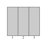
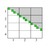
Figure 3. Using row echelon form to compute ${\mathcal{R}}_{k+1}$ from ${\mathcal{R}}_{k}$.

It is evident in the figure that $R^{k}_{i}$ maps onto $R^{k+1}_{i}$ for all $i$.

Case $N$: the matrix $N_{k}$ represents a linear map $V_{k+1}\to V_{k}$. We assume that ${\mathcal{B}}_{k}$ is compatible with the filtration ${\mathcal{R}}_{k}$, and that $\phi_{i}$ identifies the filtration. This time we have a vertical block structure

$$N_{k}=\left[\begin{array}[]{c}L_{1}\\ L_{2}\\ \vdots\\ L_{k}\end{array}\right]$$

where $L_{i}$ gathers together the rows $q$ with $\phi_{k}(q)=i$. Using column operations only, put $N_{k}$ into the column echelon form defined as follows (this echelon form begins on the bottom left):

• Each of the leftmost $r$ columns contains a 1 (the pivot) as its lowest nonzero entry.

• Each pivot lies strictly lower than the pivots of the columns to the right of it.

• The rightmost $a_{k+1}-r$ rows are entirely zero.

These column operations correspond to elementary operations $E_{k+1}(p,q,\lambda)$, and the effect of these operations is felt on the next matrix $M_{k+1}$ or $N_{k+1}$, which must be modified accordingly. We now define $\phi_{k+1}$ as follows:

$$\phi_{k+1}(p)=\left\{\begin{array}[]{ll}\phi_{k}(q)+1&\qquad\mbox{if column~{}$p$ has a pivot in row~{}$q$,}\\ 1&\qquad\mbox{if column~{}$p$ has no pivot.}\end{array}\right.$$

See Figure 4.

  

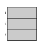
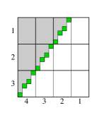
Figure 4. Using column echelon form to compute ${\mathcal{R}}_{k+1}$ from ${\mathcal{R}}_{k}$.

It is evident in the figure that $R^{k+1}_{i+1}$ is the largest subspace which maps into $R^{k}_{i}$, for all $i$.

This concludes our treatment of the concrete form of the zigzag algorithm.

5. Further Algebraic Techniques

5.1. Localization at a single index

Let ${\mathbb{V}}$ be a zigzag module of length $n$ and let $1\leq k\leq n$. We consider the problem of determining the set of intervals in $\operatorname{Pers}({\mathbb{V}})$ which contain $k$, without necessarily computing $\operatorname{Pers}({\mathbb{V}})$ itself. We shall see that all the necessary information is contained in a pair of filtrations on the vector space $V_{k}$.

Definition 5.1.

Let ${\mathbb{V}}$ be a zigzag module of length $n$. The left-filtration of ${\mathbb{V}}$ is a filtration on $V_{1}$ of depth $n$, defined as

$$\mathrm{L}({\mathbb{V}})=\mathrm{R}(\bar{{\mathbb{V}}})$$

where $\bar{\mathbb{V}}$ is the reversal of ${\mathbb{V}}$; so $\bar{V}_{i}=V_{n+1-i}$, with maps $\bar{f}_{i}=g_{n-i}$ or $\bar{g}_{i}=f_{n-i}$.

For any $k$ we therefore have two natural filtrations on $V_{k}$:

$$\begin{array}[]{rclcl}{\mathcal{R}}_{k}&=&(R_{0},R_{1},\dots,R_{k})&=&\mathrm{R}({\mathbb{V}}[1,k]),\\ {\mathcal{L}}_{k}&=&(L_{0},L_{1},\dots,L_{n+1-k})&=&\mathrm{L}({\mathbb{V}}[k,n]);\end{array}$$

the right-filtration over the index set $\{1,\dots,k\}$ and the left-filtration over the index set $\{k,\dots,n\}$. We also have birth-time and death-time indices

$$\begin{array}[]{rclcl}\mathrm{b}_{k}&=&(b_{1},\dots,b_{k})&=&\mathrm{b}(\tau[1,k])\\ \mathrm{d}_{k}&=&(d_{1},\dots,d_{n+1-k})&=&n+1-\mathrm{b}(\bar{\tau}[k,n])\end{array}$$

which indicate the birth and death times associated with the respective subquotients of ${\mathcal{R}}_{k}$ and ${\mathcal{L}}_{k}$. These depend on the type $\tau$ of ${\mathbb{V}}$.

Example 5.2.

Consider the zigzag module

$${\mathbb{V}}\;=\;(\,V_{1}\stackrel{{\scriptstyle f_{1}}}{{\longrightarrow}}V_{2}\stackrel{{\scriptstyle f_{2}}}{{\longrightarrow}}V_{3}\stackrel{{\scriptstyle g_{3}}}{{\longleftarrow}}V_{4}\,).$$

At $k=2$, for instance, we have

$$\begin{array}[]{rcl}{\mathcal{R}}_{2}&=&(0,f_{1}(V_{1}),V_{2})\\ {\mathcal{L}}_{2}&=&(0,f_{2}^{-1}(0),f_{2}^{-1}g_{3}(V_{4}),V_{2})\end{array}$$

and

$$\begin{array}[]{rcl}\mathrm{b}_{2}&=&(1,2)\\ \mathrm{d}_{2}&=&(2,4,3).\end{array}$$

We can now state the main theorem of this section.

Theorem 5.3 (Localization at index $k$).

Let ${\mathbb{V}}$ be a zigzag module of length $n$ and let $1\leq k\leq n$. Let ${\mathcal{R}}_{k},{\mathcal{L}}_{k}$ denote the right- and left-filtrations at $k$, and let $\mathrm{b}_{k},\mathrm{d}_{k}$ denote the birth-time and death-time indices at $k$. Then, for all $i,j$ in the range $1\leq i\leq k$, $1\leq j\leq n+1-k$, the multiplicity of $[b_{i},d_{j}]$ in $\operatorname{Pers}({\mathbb{V}})$ is equal to

$$c_{ij}=\dim(R_{i}\cap L_{j})-\dim(R_{i-1}\cap L_{j})-\dim(R_{i}\cap L_{j-1})+\dim(R_{i-1}\cap L_{j-1}).$$

Remark.

Equivalently, $c_{ij}=\dim((R_{i}\cap L_{j})/((R_{i-1}\cap L_{j})+(R_{i}\cap L_{j-1})))$, the dimension of the $(i,j)$-th bifiltration subquotient.

This theorem answers the original question, because every interval containing $k$ can be written as $[b_{i},d_{j}]$ for some choice of $i,j$. We now work towards a proof of Theorem 5.3.

Proposition 5.4.

It is sufficient to prove Theorem 5.3 in the special case where ${\mathbb{V}}$ is right-streamlined over $\{1,\dots,k\}$ and left-streamlined over $\{k,\dots,n\}$.

Proof.

It is clear from Lemma 4.3 that we can write ${\mathbb{V}}={\mathbb{U}}\oplus{\mathbb{W}}$ where ${\mathbb{U}}$ is supported in $\{1,\dots,k-1\}$ and ${\mathbb{W}}$ is right-streamlined over $\{1,\dots,k\}$. Indeed, take ${\mathbb{U}}={\mathbb{V}}^{1}\oplus\dots\oplus{\mathbb{V}}^{k-1}$ and ${\mathbb{W}}={\mathbb{V}}^{k}\oplus\dots\oplus{\mathbb{V}}^{n}$. Moreover, it is sufficient to prove Theorem 5.3 for ${\mathbb{W}}$, because the filtrations ${\mathcal{R}}_{k},{\mathcal{L}}_{k}$ remain unchanged from ${\mathbb{V}}$, and the discarded term ${\mathbb{U}}$ decomposes into intervals which do not contain $k$. Thus, we may assume that ${\mathbb{V}}$ is right-streamlined over $\{1,\dots,k\}$.

Repeating this argument from the other side, we may further assume that ${\mathbb{V}}$ is left-streamlined over $\{k,\dots,n\}$. ∎

Proof of Theorem 5.3.

Assume that ${\mathbb{V}}$ satisfies the condition in Proposition 5.4. It follows that every interval in $\operatorname{Pers}({\mathbb{V}})$ contains $k$: any other interval in the decomposition would cause a failure of the streamline condition. We can therefore write the interval decomposition of ${\mathbb{V}}$ as

$${\mathbb{V}}=\bigoplus_{a\in A}{\mathbb{I}}_{a}\cong\bigoplus_{a\in A}{\mathbb{I}}(b_{p(a)},d_{q(a)})$$

where $A$ indexes the summands, and $p:A\to\{1,\dots,k\}$ and $q:A\to\{1,\dots,n-k+1\}$ identify the interval type of each summand in terms of the birth-time and death-time indices. It is apparent from this formulation that

$$c_{ij}=\#\{a\in A\mid p(a)=i,\,q(a)=j\}$$

and it remains to compute this in terms of the dimensions $\dim(R_{i}\cap L_{j})$.

The interval decomposition restricts at index $k$ to a direct sum decomposition of $V_{k}$ into 1-dimensional subspaces $U_{a}$, generated by elements $x_{a}$, say. Then

$${\mathcal{R}}_{k}=\bigoplus_{a\in A}\mathrm{R}({\mathbb{I}}_{a}[1,k])=\bigoplus_{a\in A}{\mathcal{R}}_{k}\cap U_{a}\cong\bigoplus_{a\in A}{\mathcal{J}}(p(a),k)$$

where the final isomorphism comes from Lemma 3.9. Now, the filtration subspace $R_{i}$ is spanned by the terms isomorphic to ${\mathcal{J}}(p,k)$ with $p\leq i$. In other words, for $i=1,\dots,k$ we have

$$R_{i}=\operatorname{Span}\left\{x_{a}\mid p(a)\leq i\right\}.$$

A similar argument proceeding from the other direction gives the analogous formula

$$L_{j}=\operatorname{Span}\left\{x_{a}\mid q(a)\leq j\right\},$$

for $j=1,\dots,n+1-k$. Since the $x_{a}$ are independent, these formulas give bases for $R_{i},L_{j}$.

We now claim that

$$R_{i}\cap L_{j}=\operatorname{Span}\{x_{a}\mid p(a)\leq i,\,q(a)\leq j\}$$

for all $i,j$. The inclusion $\operatorname{Span}\subseteq R_{i}\cap L_{j}$ is obvious, because each of the spanning vectors $x_{a}$ belongs to both $R_{i}$ and $L_{j}$. In the other direction, if $x\in R_{i}\cap L_{j}$ then write $x=\sum_{a\in A}\lambda_{a}x_{a}$. Since $x\in R_{i}$, all the coefficients $\lambda_{a}$ with $p(a)>i$ must be zero. Since $x\in L_{j}$, all the coefficients $\lambda_{a}$ with $q(a)>j$ must be zero. Thus $x\in\operatorname{Span}\{x_{a}\mid p(a)\leq i,\,q(a)\leq j\}$. This establishes the reverse inclusion $R_{i}\cap L_{j}\subseteq\operatorname{Span}$ and hence the equality.

Then

$$\dim(R_{i}\cap L_{j})=\#\{x_{a}\mid p(a)\leq i,\,q(a)\leq j\}=\sum_{p=1}^{i}\sum_{q=1}^{j}c_{pq}$$

for all $i,j$. The formula in the theorem follows easily from this. ∎

Remark.

The salient fact behind this result is that it is possible to find a direct sum decomposition of $V_{k}$ which simultaneously decomposes the filtered spaces ${\mathcal{R}}_{k},{\mathcal{L}}_{k}$ into intervals within their respective categories $\operatorname{Filt}_{k}$, $\operatorname{Filt}_{n+1-k}$. Here we achieved this by appealing to the interval decomposition of ${\mathbb{V}}$, but this can also be proved directly for an arbitrary pair of filtrations on a single vector space. The analogous statement for a triple of filtrations is false. For example

$$(0,\mathbb{F}\oplus 0,\mathbb{F}^{2}),\qquad(0,0\oplus\mathbb{F},\mathbb{F}^{2}),\qquad(0,\Delta,\mathbb{F}^{2}),$$

(where $\Delta=\{(x,x)\mid x\in\mathbb{F}\}$) cannot be simultaneously decomposed into intervals.

5.2. The Diamond Principle

Consider the following diagram:

$$\begin{diagram}$$

Let ${\mathbb{V}}^{+}$ and ${\mathbb{V}}^{-}$ denote the two zigzag modules contained in the diagram:

$${\mathbb{V}}^{+} = (\,V_{1}\longleftrightarrow\dots\longleftrightarrow V_{k-1}\stackrel{{\scriptstyle f_{k-1}}}{{\longrightarrow}}W_{k}\stackrel{{\scriptstyle g_{k}}}{{\longleftarrow}}V_{k+1}\longleftrightarrow\dots\longleftrightarrow V_{n}\,)$$

$${\mathbb{V}}^{-} = (\,V_{1}\longleftrightarrow\dots\longleftrightarrow V_{k-1}\stackrel{{\scriptstyle g_{k-1}}}{{\longleftarrow}}U_{k}\stackrel{{\scriptstyle f_{k}}}{{\longrightarrow}}V_{k+1}\longleftrightarrow\dots\longleftrightarrow V_{n}\,)$$

We wish to compare $\operatorname{Pers}({\mathbb{V}}^{+})$ with $\operatorname{Pers}({\mathbb{V}}^{-})$, particularly with respect to intervals that meet $\{k-1,k,k+1\}$. This requires a favourable condition on the four maps in the middle diamond.

Definition 5.5.

We say that the diagram

$$\begin{diagram}$$

is exact if $\operatorname{Im}(D_{1})=\operatorname{Ker}(D_{2})$ in the following sequence

$$\begin{diagram}$$

where $D_{1}(u)=g_{k-1}(u)\oplus f_{k}(u)$ and $D_{2}(v\oplus v^{\prime})=f_{k-1}(v)-g_{k}(v^{\prime})$.

Theorem 5.6 (The Diamond Principle).

Given ${\mathbb{V}}^{+}$ and ${\mathbb{V}}^{-}$ as above, suppose that the middle diamond is exact. Then there is a partial bijection of the multisets $\operatorname{Pers}({\mathbb{V}}^{+})$ and $\operatorname{Pers}({\mathbb{V}}^{-})$, with intervals matched according to the following rules:

• Intervals of type $[k,k]$ are unmatched.

• Type $[b,k]$ is matched with type $[b,k-1]$ and vice versa, for $b\leq k-1$.

• Type $[k,d]$ is matched with type $[k+1,d]$ and vice versa, for $d\geq k+1$.

• Type $[b,d]$ is matched with type $[b,d]$, in all other cases.

It follows that the restrictions $\operatorname{Pers}({\mathbb{V}}^{+})|_{K}$, $\operatorname{Pers}({\mathbb{V}}^{-})|_{K}$ to the set $K=\{1,\dots,n\}\setminus\{k\}$ are equal.

Figures 5 and 6 illustrate Theorem 5.6 in terms of barcodes and persistence diagrams, respectively.

Figure 5. Interval matching between $\operatorname{Pers}({\mathbb{V}}^{+})$ and $\operatorname{Pers}({\mathbb{V}}^{-})$: (top row) the five cases where matching occurs; (bottom row) unmatched intervals $[k,k]$.

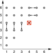
Figure 6. From $\operatorname{Pers}({\mathbb{V}}^{+})$ to $\operatorname{Pers}({\mathbb{V}}^{-})$, for $n=6$, $k=4$: points in the persistence plane move according to the arrows; the multiplicity of the point marked $\boxtimes$ changes unpredictably.

Remark.

The ${\mathbb{I}}(k,k)$ summands in $\operatorname{Pers}({\mathbb{V}}^{+})$ span the cokernel of $D_{2}$, whereas the ${\mathbb{I}}(k,k)$ summands in $\operatorname{Pers}({\mathbb{V}}^{-})$ span the kernel of $D_{1}$. The hypothesis of Theorem 5.6 does not bring about any relation between these spaces (which is why the $[k,k]$ intervals are unmatched). In Section 5.3, however, we consider a situation in which the $[k,k]$ intervals can be tracked.

We use the localization technique of Section 5.1 to prove Theorem 5.6. We begin with birth- and death-time indices.

Proposition 5.7.

Let $\tau^{+},\tau^{-}$ denote the zigzag types of ${\mathbb{V}}^{+},{\mathbb{V}}^{-}$ respectively. If we write

$$(b_{1},\dots,b_{k-1})=\mathrm{b}(\tau^{+}[1,k-1])=\mathrm{b}(\tau^{-}[1,k-1])$$

for the birth-time index up to time $k-1$, then

$$\mathrm{b}(\tau^{+}[1,k+1]) = (k+1,b_{1},\dots,b_{k-1},k).$$

$$\mathrm{b}(\tau^{-}[1,k+1]) = (k,b_{1},\dots,b_{k-1},k+1),$$

Similarly, if we write

$$(d_{1},\dots,d_{n-k})=\mathrm{d}(\tau^{+}[k+1,n])=\mathrm{d}(\tau^{-}[k+1,n])$$

for the death-time index from time $k+1$, then

$$\mathrm{d}(\tau^{+}[k-1,n]) = (k-1,d_{1},\dots,d_{n-k},k).$$

$$\mathrm{d}(\tau^{-}[k-1,n]) = (k,d_{1},\dots,d_{n-k},k-1),$$

Proof.

This is immediate from the recursive definition of birth-time index. If we write $\tau_{0}=\tau^{+}[1,k-1]=\tau^{-}[1,k-1]$ then $\tau^{+}[1,k+1]=\tau_{0}fg$ and $\tau^{-}[1,k+1]=\tau_{0}gf$. The death-time index is treated similarly. ∎

Here is the crux of the matter:

Lemma 5.8.

In the situation of Theorem 5.6, the following filtrations are equal:

$$\mathrm{R}({\mathbb{V}}^{+}[1,k+1]) = \mathrm{R}({\mathbb{V}}^{-}[1,k+1])$$

$$\mathrm{L}({\mathbb{V}}^{+}[k-1,n]) = \mathrm{L}({\mathbb{V}}^{-}[k-1,n])$$

Proof.

Write $(R_{0},R_{1},\dots,R_{k-1})=\mathrm{R}({\mathbb{V}}^{+}[1,k-1])=\mathrm{R}({\mathbb{V}}^{-}[1,k-1])$. By the recursive formula (Definition 3.1),

$$\mathrm{R}({\mathbb{V}}^{+}[1,k+1])=(0,g_{k}^{-1}f_{k-1}(R_{0}),\dots,g_{k}^{-1}f_{k-1}(R_{k-1}),V_{k+1})$$

and

$$\mathrm{R}({\mathbb{V}}^{-}[1,k+1])=(0,f_{k}g_{k-1}^{-1}(R_{0}),\dots,f_{k}g_{k-1}^{-1}(R_{k-1}),V_{k+1}).$$

Thus we can prove the first statement of the lemma by showing that

$$f_{k}g_{k-1}^{-1}(R)=g_{k}^{-1}f_{k-1}(R)$$

for any subspace $R\leq V_{k-1}$. We use first-order logic. Let $x\in V_{k+1}$. We have the following chain of equivalent statements.

$$x\in f_{k}g_{k-1}^{-1}(R)$$

$$\Leftrightarrow (\exists z\in R)\,(\exists y\in U_{k})\,((g_{k-1}(y)=z)\,\&\,(f_{k}(y)=x))$$

$$\Leftrightarrow (\exists z\in R)\,(\exists y\in U_{k})\,(D_{1}(y)=z\oplus x)$$

$$\Leftrightarrow (\exists z\in R)\,(z\oplus x\in\operatorname{Im}(D_{1}))$$

On the other hand:

$$x\in g_{k}^{-1}f_{k-1}(R)$$

$$\Leftrightarrow (\exists z\in R)\,(f_{k-1}(z)=g_{k}(x))$$

$$\Leftrightarrow (\exists z\in R)\,(z\oplus x\in\operatorname{Ker}(D_{2}))$$

Since $\operatorname{Im}(D_{1})=\operatorname{Ker}(D_{2})$ by hypothesis, it follows that $f_{k}g_{k-1}^{-1}(R)=g_{k}^{-1}f_{k-1}(R)$.

This proves the first equality. The second equality follows symmetrically. ∎

Proof of Theorem 5.6.

We adopt the notation of Section 5.1, and consider the right- and left-filtrations at $V_{k+1}$, for both ${\mathbb{V}}^{+}$ and ${\mathbb{V}}^{-}$. Since ${\mathbb{V}}^{+}[k+1,n]={\mathbb{V}}^{-}[k+1,n]$ we have

$${\mathcal{L}}_{k+1}^{+}={\mathcal{L}}_{k+1}^{-}\qquad\mbox{and}\qquad\mathrm{d}_{k+1}^{+}=\mathrm{d}_{k+1}^{-},$$

and by Lemma 5.8 we have

$${\mathcal{R}}_{k+1}^{+}={\mathcal{R}}_{k+1}^{-}.$$

Finally, $\mathrm{b}_{k+1}^{+}$ agrees with $\mathrm{b}_{k+1}^{-}$ except that $k,k+1$ are interchanged, according to Proposition 5.7. Thus, when we use Theorem 5.3 to calculate the multiplicity of $[b,d]$ for $b\leq k+1\leq d$, there is perfect agreement between ${\mathbb{V}}^{+}$ and ${\mathbb{V}}^{-}$ except that we must interchange $k,k+1$ when they occur as birth-times.

A symmetrical argument can be made, localizing at $V_{k-1}$. When we compute the multiplicity of $[b,d]$ for $b\leq k-1\leq d$, there is perfect agreement between ${\mathbb{V}}^{+}$ and ${\mathbb{V}}^{-}$ except that we must interchange $k,k-1$ when they occur as death-times.

We have covered all cases of the theorem except for intervals which meet neither $k-1$ nor $k+1$. Intervals contained in $[1,k-2]$ are automatically the same for ${\mathbb{V}}^{+}$ and ${\mathbb{V}}^{-}$ because they can be computed by restricting to ${\mathbb{V}}^{+}[1,k-1]$ and ${\mathbb{V}}^{-}[1,k-1]$, which are equal. Similarly, intervals contained in $[k+2,n]$ are the same for ${\mathbb{V}}^{+}$ and ${\mathbb{V}}^{-}$, by restricting to ${\mathbb{V}}^{+}[k+1,n]={\mathbb{V}}^{-}[k+1,n]$.

Finally, consider intervals $[k,k]$. Nothing can be said about those. ∎

5.3. The Strong Diamond Principle

The Diamond Principle can usefully be applied to the following diagram of topological spaces and continuous maps. The four maps in the central diamond are inclusion maps, and the remaining maps $\leftrightarrow$ are arbitrary.

$$\begin{diagram}$$

Let ${\mathbb{X}}^{+},{\mathbb{X}}^{-}$ denote the upper and lower zigzag diagrams contained in this picture; so ${\mathbb{X}}^{+}$ passes through $A\cup B$ and ${\mathbb{X}}^{-}$, passes through $A\cap B$.

Theorem 5.9 (The Strong Diamond Principle).

Given ${\mathbb{X}}^{+}$ and ${\mathbb{X}}^{-}$ as above, there is a (complete) bijection between the multisets $\operatorname{Pers}(H_{*}({\mathbb{X}}^{+}))$ and $\operatorname{Pers}(H_{*}({\mathbb{X}}^{-}))$. Intervals are matched according to the following rules:

• $[k,k]\in\operatorname{Pers}(H_{\ell+1}({\mathbb{X}}^{+}))$ is matched with $[k,k]\in\operatorname{Pers}(H_{\ell}({\mathbb{X}}^{-}))$.

In the remaining cases, the matching preserves homological dimension:

• Type $[b,k]$ is matched with type $[b,k-1]$ and vice versa, for $b\leq k-1$.

• Type $[k,d]$ is matched with type $[k+1,d]$ and vice versa, for $d\geq k+1$.

• Type $[b,d]$ is matched with type $[b,d]$, in all other cases.

Proof.

For any $\ell$, apply the homology functor $H_{\ell}$ to the diagram. The central diamond

$$\begin{diagram}$$

is exact by virtue of the Mayer–Vietoris theorem, according to which

$$\ldots\longrightarrow H_{\ell}(A\cap B)\stackrel{{\scriptstyle D_{1}}}{{\longrightarrow}}H_{\ell}(A)\oplus H_{\ell}(B)\stackrel{{\scriptstyle D_{2}}}{{\longrightarrow}}H_{\ell}(A\cup B)\longrightarrow\ldots$$

is an exact sequence. The Diamond Principle therefore applies to $H_{\ell}({\mathbb{X}}^{+})$ and $H_{\ell}({\mathbb{X}}^{-})$, and we have a partial bijection which accounts for all intervals except those of type $[k,k]$.

Now consider the connecting homomorphism in the same Mayer–Vietoris sequence:

$$\ldots\stackrel{{\scriptstyle D_{2}}}{{\longrightarrow}}H_{\ell+1}(A\cup B)\stackrel{{\scriptstyle\partial}}{{\longrightarrow}}H_{\ell}(A\cap B)\stackrel{{\scriptstyle D_{1}}}{{\longrightarrow}}\ldots$$

By exactness, $\partial$ induces an isomorphism between the cokernel of $D_{2}$ and the kernel of $D_{1}$. But the $[k,k]$ summands of $\operatorname{Pers}(H_{\ell+1}({\mathbb{X}}^{+}))$ precisely span $\operatorname{Coker}(D_{2})$, whereas the $[k,k]$ summands of $\operatorname{Pers}(H_{\ell}({\mathbb{X}}^{-}))$ span $\operatorname{Ker}(D_{1})$. This establishes the claimed bijection between the $[k,k]$ intervals. ∎

Example 5.10.

Let ${\mathbb{X}}=(X_{1},\dots,X_{n})$ be a sequence of simplicial complexes defined on a common vertex set. Suppose these have arisen in some context where each transition $X_{i}$ to $X_{i+1}$ is regarded as being a ‘small’ change. There are two natural zigzag sequences linking the $X_{i}$.

The union zigzag, ${\mathbb{X}}_{\cup}$:

$$\begin{diagram}$$

The intersection zigzag, ${\mathbb{X}}_{\cap}$:

$$\begin{diagram}$$

We can think of these as being indexed by the half-integers $\{1,1\frac{1}{2},2,2\frac{1}{2},\dots,n\}$.

We can apply the Strong Diamond Principle $n-1$ times to derive the following relationship between the zigzag persistence of the two sequences $\operatorname{Pers}(H_{\ell}({\mathbb{X}}_{\cap}))$ and $\operatorname{Pers}(H_{\ell}({\mathbb{X}}_{\cup}))$. Restricting to the integer indices, there is a coarse equality:

$$\operatorname{Pers}(H_{\ell}({\mathbb{X}}_{\cup}))|_{\{1,\dots,n\}}=\operatorname{Pers}(H_{\ell}({\mathbb{X}}_{\cap}))|_{\{1,\dots,n\}}$$

More finely, there is a partial bijection between $\operatorname{Pers}(H_{\ell}({\mathbb{X}}_{\cup}))$ and $\operatorname{Pers}(H_{\ell}({\mathbb{X}}_{\cap}))$. Intervals $[k\frac{1}{2},k\frac{1}{2}]$ shift homological dimension by $+1$ (from the intersection sequence to the union sequence). Otherwise $[b,d]\leftrightarrow[b^{\prime},d^{\prime}]$ where $\{b,b^{\prime}\}$ is an unordered pair of the form $\{k\frac{1}{2},k+1\}$ and $\{d,d^{\prime}\}$ is an unordered pair of the form $\{k,k\frac{1}{2}\}$; dimension is preserved. Figure 7 illustrates the complete correspondence as a transformation of the persistence diagram, for $n=5$.

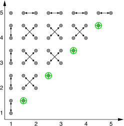
Figure 7. From $\operatorname{Pers}(H_{*}({\mathbb{X}}_{\cap}))$ to $\operatorname{Pers}(H_{*}({\mathbb{X}}_{\cup}))$, for $n=5$: points in the persistence plane move according to the arrows; points marked $\oplus$ stay fixed and increase homological dimension by 1.

Concluding Remarks

We have presented the foundations of a theory of zigzag persistence which, we believe, considerably extends and enriches the well known and highly successful theory of persistent homology. Zigzag persistence originates in the work of Gabriel and others in the theory of quiver representations. One of our goals has been to bridge the gap between the quiver literature (which is read largely by algebraists) and the current language of applied and computational topology. To this end, we have presented an algorithmic form of Gabriel’s structure theorem for $A_{n}$ quivers, and have indicated the first steps towards integrating these ideas into tools for applied topology.

There are several ways in which this work is incomplete. The most significant omission is an algorithm for computing zigzag persistence in a homological setting (as distinct from the somewhat sanitised vector space algorithm described in Section 4.3). We address this gap in a forthcoming paper with Dmitriy Morozov [C_dS_M_2008], where we present an algorithm for computing the zigzag persistence intervals of a 1-parameter family of simplicial complexes on a fixed vertex set.

We have made no effort in this paper to flesh out the applications suggested in Section 1. There is often a substantial gap between the concrete world of point-cloud data sets and the ideal world of simplicial complexes and topological spaces. We intend to develop some of these applications in future work. Meanwhile, we have given priority to establishing the theoretical language and tools. The Diamond Principle is particularly powerful. In the manuscript with Morozov [C_dS_M_2008], we show that the Diamond Principle can be used to establish isomorphisms between several different classes of persistence invariants of a space with a real-valued (e.g. Morse) function. In particular, we use zigzag persistence to resolve an open conjecture concerning extended persistence [CS_E_H_2008]. This supports our prejudice that zigzag persistence provides the appropriate level of generality and power for understanding the heuristic concept of persistence in its many manifestations.

Acknowledgements

The authors wish to thank Greg Kuperberg, Konstantin Mischaikow and Dmitriy Morozov for helpful conversations and M. Khovanov for helpful correspondence. The authors gratefully acknowledge support from DARPA, in the form of grants HR0011-05-1-0007 and HR0011-07-1-0002. The second author wishes to thank Pomona College and Stanford University for, respectively, granting and hosting his sabbatical during late 2008.