Localization in Correlated Bi-Layer Structures:
From Photonic Cristals to Metamaterials and Electron Superlattices

Abstract

In a unified approach, we study the transport properties of periodic-on-average bi-layered photonic crystals, metamaterials and electron superlattices. Our consideration is based on the analytical expression for the localization length derived for the case of weakly fluctuating widths of layers, that also takes into account possible correlations in disorder. We analyze how the correlations lead to anomalous properties of transport. In particular, we show that for quarter stack layered media specific correlations can result in a $\omega^{2}$-dependence of the Lyapunov exponent in all spectral bands.

Introduction. In recent years much attention was paid to the propagation of waves (electrons) in periodic one-dimensional structures (see, e.g. MS08 and references therein). The interest to this subject is due to various applications in which one needs to create materials, metamaterials or electron superlattices with given transmission properties. One of the important problems that still remains open, is the influence of a disorder that can not be avoided in experimental devices. Such a disorder can be manifested by fluctuations of the width of layers and distance between layers, or due to variations of the medium parameters, such as dielectric constant, magnetic permeability or barrier hight (for electrons) MCMM93 ; So00 ; SSS01 ; Po03 ; Eo06 ; No07 ; Po07 ; Ao07 .

As is well known, the main quantity that absorbs the influence of a disorder is the localization length entirely determining transport properties in a 1D geometry LGP88 . In contrast to many studies of the wave (electron) propagation through random structures, mainly based on various numerical methods, in this Letter we develop an analytical approach allowing us to derive the unique expression for the localization length that is valid for photonic crystals, metamaterials and electron superlattices. Another key point of consideration is that we explicitly take into account possible correlations within a disorder, that may be imposed experimentally. As was recently shown, both theoretically IK99 ; IKU01 ; IM ; HIT08 and experimentally Bo99 ; KIKS00 , specific long-range correlations can significantly enhance or suppress the localization length in desired windows of frequency of incident waves.

Model. We consider the propagation of electromagnetic wave of the frequency $\omega$ through an infinite array of two alternating $a$ and $b-$layers (slabs). The slabs are specified by the dielectric constant $\varepsilon_{a,b}$, magnetic permeability $\mu_{a,b}$, refractive index $n_{a,b}=\sqrt{\varepsilon_{a,b}\mu_{a,b}}$, impedance $Z_{a,b}=\sqrt{\mu_{a,b}/\varepsilon_{a,b}}$ and wave number $k_{a,b}=\omega n_{a,b}/c$. We assume that the $z$-axis is directed along the array of bi-layers perpendicular to the stratification. Within the layers, the electric field obeys the wave equation,

$$\left(\frac{d^{2}}{dz^{2}}+k_{a,b}^{2}\right)\psi_{a,b}(z)=0,$$ (1)

with two boundary conditions on the interfaces $z=z_{i}$ between slabs, $\psi_{a}(z_{i})=\psi_{b}(z_{i})$ and $\mu_{a}^{-1}\psi^{\prime}_{a}(z_{i})=\mu_{b}^{-1}\psi^{\prime}_{b}(z_{i})$.

A disorder is incorporated in the structure via the random widths of the slabs, $\widetilde{a}(n)=a+\varrho_{a}(n)$, $\widetilde{b}(n)=b+\varrho_{b}(n)$. Here $n$ enumerates the elementary $ab$-cells, $a$ and $b$ are the average widths of layers and $\varrho_{a}(n)$, $\varrho_{b}(n)$ stand for small variations of the widths. In the absence of disorder the array of slabs is periodic with the period $d=a+b$. The random sequences $\varrho_{a,b}(n)$ are supposed to be statistically homogeneous with zero average, $\langle\varrho_{a,b}(n)\rangle=0$, and the correlations are fully determined by the binary correlation functions

$$\langle\varrho_{j}(n)\varrho_{j}(n^{\prime})\rangle=\langle\varrho^{2}_{j}(n)\rangle K_{j}(n-n^{\prime}),\,\,\,\,j=a,b$$ (2)

$$\langle\varrho_{a}(n)\varrho_{b}(n^{\prime})\rangle=\langle\varrho_{a}(n)\varrho_{b}(n)\rangle K_{ab}(n-n^{\prime}).$$ (3)

In what follows the average $\langle...\rangle$ is performed over the whole array of layers or due to the ensemble averaging, that is assumed to be the same. The two-point auto-correlators $K_{a,b}(n-n^{\prime})$ as well as the inter-correlator $K_{ab}(n-n^{\prime})$ are normalized to one, $K_{a,b}(0)=K_{ab}(0)=1$. The variances $\langle\varrho^{2}_{a,b}(n)\rangle$ are of positive value, while $\langle\varrho_{a}(n)\varrho_{b}(n)\rangle$ can be both positive and negative. Note that $|\langle\varrho_{a}(n)\varrho_{b}(n)\rangle|=\sqrt{\langle\varrho^{2}_{a}(n)\rangle\langle\varrho^{2}_{b}(n)\rangle}$. We assume the positional disorder be weak, $k^{2}_{a,b}\langle\varrho^{2}_{a,b}(n)\rangle\ll 1$, allowing us to use an appropriate perturbation theory. In this case, all transport properties are entirely determined by the randomness power spectra $\mathcal{K}_{a}(k)$, $\mathcal{K}_{b}(k)$, and $\mathcal{K}_{ab}(k)$, defined by the relation, $\mathcal{K}(k)=\sum_{r=-\infty}^{\infty}K(r)\exp(-ikr)$. All the correlators $K(r)$ are real and even functions of the difference $r=n-n^{\prime}$. Because of this fact and due to their positive normalization, the corresponding Fourier transforms $\mathcal{K}(k)$ are real, even and non-negative functions of the dimensionless lengthwise wave-number $k$.

Method. Our aim is to derive the localization length (LL) $l_{\infty}(\omega)$ in the general case of either white or colored disorder. On the scale of individual slabs the solution of Eq. (1) can be presented in the form of two maps for $n$th $a$ and $b$ layer, respectively, with corresponding phase shifts $\widetilde{\varphi}_{a,b}(n)=\varphi_{a,b}+\xi_{a,b}(n)$, where $\varphi_{a}=k_{a}a$, $\varphi_{b}=k_{b}b$, and $\xi_{a,b}(n)=k_{a,b}\varrho_{a,b}(n)$. By combining these maps with the use of the boundary conditions, one can write the map for the whole $n$th elementary $ab$-cell,

$$x_{n+1}=\widetilde{A}_{n}x_{n}+\widetilde{B}_{n}y_{n},\qquad y_{n+1}=-\widetilde{C}_{n}x_{n}+\widetilde{D}_{n}y_{n}.$$ (4)

Here $x_{n}=\psi_{a}(z_{an})$ and $y_{n}=k_{a}^{-1}\psi^{\prime}_{a}(z_{an})$, the index $n$ corresponds to the left edge while $n+1$ stands for the right edge of the $n$th cell. The constants $\widetilde{A}_{n}$, $\widetilde{B}_{n}$, $\widetilde{C}_{n}$, $\widetilde{D}_{n}$ depend on $\widetilde{\varphi}_{a}(n)$, $\widetilde{\varphi}_{b}(n)$ and on $Z_{a}/Z_{b}=k_{b}\mu_{a}/k_{a}\mu_{b}$.

Eq. (4) can be treated as the map of a linear oscillator with time-dependent parametric force IKT95 . Without disorder the trajectory $x_{n},y_{n}$ creates an ellipse in the phase space $(x,y)$, that is an image of the unperturbed motion. It is convenient to make the transformation, $x_{n}=\upsilon^{-1}Q_{n}\cos\tau-\upsilon P_{n}\sin\tau$, $y_{n}=\upsilon^{-1}Q_{n}\sin\tau+\upsilon P_{n}\cos\tau$, to new coordinates $Q_{n},P_{n}$, in which the unperturbed trajectory occupies the circle, $Q_{n+1}=Q_{n}\cos\gamma+P_{n}\sin\gamma$, $P_{n+1}=-Q_{n}\sin\gamma+P_{n}\cos\gamma$, in the phase space $(Q,P)$. Here $\tau$ and $\upsilon$ can be found from Eq. (4), and $\gamma$ determines the Bloch wave number $\kappa=\gamma/d$ arising in the relation $\psi(z+d)=\exp(i\kappa d)\psi(z)$ for the periodic array,

$$\cos\gamma=\cos\varphi_{a}\cos\varphi_{b}-\frac{1}{2}\left(\frac{Z_{b}}{Z_{a}}+\frac{Z_{a}}{Z_{b}}\right)\sin\varphi_{a}\sin\varphi_{b}.$$ (5)

In order to take into account the disorder, we expand the constants $\widetilde{A}_{n}$, $\widetilde{B}_{n}$, $\widetilde{C}_{n}$, $\widetilde{D}_{n}$ up to the second order in the perturbation parameters $\xi_{a}(n)\ll 1$ and $\xi_{b}(n)\ll 1$. Then, one can transform the variables $x_{n},y_{n}$ into $Q_{n},P_{n}$. After getting the perturbed map for $Q_{n},P_{n}$, we pass to action-angle variables $R_{n}$, $\theta_{n}$ via the standard transformations, $Q_{n}=R_{n}\cos\theta_{n}$, $P_{n}=R_{n}\sin\theta_{n}$. This allows us to derive the relation between $R_{n+1}$ and $R_{n}$ keeping linear and quadratic terms in the perturbation,

$$\frac{R_{n+1}^{2}}{R_{n}^{2}}=1+\xi_{a}(n)V_{a}(n)+\xi_{b}(n)V_{b}(n)-\xi_{a}^{2}(n)-\xi_{b}^{2}(n)$$

$$+\xi_{a}^{2}(n)W_{a}(n)+\xi_{b}^{2}(n)W_{b}(n)+\xi_{a}(n)\xi_{b}(n)W_{ab}(n),$$ (6)

where $V_{a}(n)$, $V_{b}(n)$, $W_{a}(n)$, $W_{b}(n)$, $W_{ab}(n)$ are complicated functions of $\theta_{n}$ and the model parameters.

Localization length. The LL can be expressed via the Lyapunov exponent (LE) $\lambda=d/l_{\infty}(\omega)$ defined by IKT95 ,

$$\lambda=\frac{1}{2}\langle\ln\left(\frac{R_{n+1}}{R_{n}}\right)^{2}\rangle.$$ (7)

In deriving the LE it was assumed that the distribution of $\theta_{n}$ is homogenous within the first order of approximation. This assumption is correct apart from the band edges, $\gamma=0;\pi$, and the vicinity of the center, $\gamma=\pi/2$ HIT08 . The calculation of the LE has been done with the use of the method developed in Refs. IK99 ; IKU01 ; HIT08 . Omitting all details, here we refer to the final result for the total LE,

$$\lambda = \frac{\varpi^{2}}{8\sin^{2}\gamma}\Big{[}\sigma^{2}_{a}\mathcal{K}_{a}(2\gamma)\sin^{2}\varphi_{b}+\sigma^{2}_{b}\mathcal{K}_{b}(2\gamma)\sin^{2}\varphi_{a}$$ (8)

$$-2\sigma^{2}_{ab}\mathcal{K}_{ab}(2\gamma)\sin\varphi_{a}\sin\varphi_{b}\cos\gamma\Big{]},$$

where $\sigma^{2}_{a,b}=k_{a,b}^{2}\langle\varrho^{2}_{a,b}(n)\rangle$, $\sigma^{2}_{ab}=k_{a}k_{b}\langle\varrho_{a}(n)\varrho_{b}(n)\rangle$, and $\varpi=Z_{a}/Z_{b}-Z_{b}/Z_{a}$ is the mismatching factor. The expression (8) generalizes the results obtained in Refs. BW85 ; IKU01 ; HIT08 for particular cases, and is in a complete correspondence with them. Let us now discuss the derived expression in some applications.

Conventional Photonic Layered Media. In this case all the optical characteristics, $\varepsilon_{a,b}$, $\mu_{a,b}$, $n_{a,b}$, $Z_{a,b}$ are positive constants. One can see that if the impedances of $a,b$-slabs are equal, $Z_{a}=Z_{b}$, the mismatching factor $\varpi$ entering Eq. (8) vanishes and the perfect transparency emerges ($\lambda=0$) even in the presence of a disorder. Since the layers are perfectly matched, this conclusion is general MS08 , and does not depend on the strength of disorder. According to Eq. (5), in such a case the stack-structure is effectively equivalent to the homogeneous medium with the linear spectrum, $\kappa=\omega\overline{n}/c$, that has no gaps, and where the refractive index is $\overline{n}=(n_{a}a+n_{b}b)/(a+b)$.

For the Fabry-Perot resonances appearing when $\omega/c=s_{a}\pi/n_{a}a$ and $\omega/c=s_{b}\pi/n_{b}b$, with $s_{a,b}=1,2,3,\dots$, the factors $\sin\varphi_{a}$ and $\sin\varphi_{b}$ in Eq. (8) vanish, thus giving rise to the resonance increase of the LL. In a special case when $n_{a}a/n_{b}b=s_{a}/s_{b}$ some resonances from different layers coincide and would give rise to the divergence of the LL. However, such a situation can arise only at the edges of spectral bands, where $\gamma=0,\pi$ and $\sin^{2}\gamma$ also vanishes. Therefore, the LL gets a finite value at these points instead of diverging (due to resonances) or vanishing (due to band edges). The above statement is not valid at the bottom of the spectrum, $\omega/c=0$, where the analysis has to be done separately. Note, nevertheless, that for a white noise, $\mathcal{K}_{a,b}=1,\,\mathcal{K}_{ab}=0,\pm 1$, the LE obeys the conventional dependence $\lambda\propto\omega^{2}$ for $\omega\to 0$.

A special interest is in the long-range correlations leading to the divergence of the LL in the controlled windows of frequency $\omega$. This effect is similar to that found in more simple 1D models with the correlated disorder IK99 ; IKU01 ; HIT08 ; KIKS00 . In our model this effect is due to a possibility to have the vanishing values of all Fourier transforms, $\mathcal{K}_{a,b}=\mathcal{K}_{ab}=0$, in some range of frequency $\omega$. This fact is important in view of experimental realizations of random disorder with specific correlations. In particular, one can artificially construct an array of random bi-layers with such power spectra that abruptly vanishes within prescribed intervals of $\omega$, resulting in the divergence of the LL. Also, specific correlations DIKR08 in a disorder can be used to “kill” a sharp frequency dependence associated with the term $\sin^{2}\gamma$ in the denominator of Eq. (8). It is noteworthy that in the middle of spectral Bloch bands ($\gamma=\pi/2$), the third term vanishes and the inter-correlations do not contribute to the LL.

The typical dependence $\lambda(\omega)$ for the conventional photonic bi-layer stack is shown in Fig. 1.

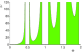
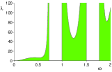
Figure 1: Lyapunov exponent $\lambda$ versus frequency $\omega$ in arbitrary units for $\varpi^{2}n_{a}^{2}\langle\varrho^{2}_{a}(n)\rangle/(2c^{2})\approx 12.28$, $\varpi^{2}n_{b}^{2}\langle\varrho^{2}_{b}(n)\rangle/(2c^{2})\approx 0.27$ and $n_{a}a/c=1.6$, $n_{b}b/c=0.4$. Left: photonic layered medium, Eqs. (8) and (5). Right: the RH-LH bi-layers with “plus” in Eq. (5).

Quarter Stack Layered Medium. This term is typically used when two basic layers, $a$ and $b$, have the same optical width, $n_{a}a=n_{b}b$ (see, e.g. MS08 ). Since $\varphi_{a}=\varphi_{b}$, in this case the dispersion relation (5) takes the form,

$$\cos\gamma=1-\frac{1}{2}\frac{(Z_{a}+Z_{b})^{2}}{Z_{a}Z_{b}}\sin^{2}(k_{a}a).$$ (9)

One can see that starting from the second band the top of every even band coincides with the bottom of next odd band at $\gamma=0$. The gaps arise only at $\gamma=\pi$.

With the use of Eq. (9) the LE can be written as

$$\lambda = \frac{\mathcal{Z}f(\gamma)}{8\cos^{2}(\gamma/2)},\qquad\mathcal{Z}=\frac{(Z_{a}-Z_{b})^{2}}{Z_{a}Z_{b}},$$ (10)

$$f(\gamma) = \sigma^{2}_{a}\mathcal{K}_{a}(2\gamma)+\sigma^{2}_{b}\mathcal{K}_{b}(2\gamma)-2\sigma_{ab}^{2}\mathcal{K}_{ab}(2\gamma)\cos\gamma.$$

Thus, the LE is finite or vanishes at $\gamma=0$ and diverges at $\gamma=\pi$.

It is instructive to analyze the simplest case of correlations when either $\xi_{a}(n)=\xi_{b}(n)$ (plus-correlations) or $\xi_{a}(n)=-\xi_{b}(n)$ (minus-correlations). In this case one gets $f(\gamma)=2\sigma^{2}_{a}\mathcal{K}_{a}(2\gamma)(1\mp\cos\gamma)$, correspondingly. As a result, for the LE one can obtain,

$$\lambda_{+}=\frac{\mathcal{Z}\sigma_{a}^{2}\mathcal{K}_{a}(2\gamma)}{2}\tan^{2}\frac{\gamma}{2};\qquad\lambda_{-}=\frac{\mathcal{Z}\sigma_{a}^{2}\mathcal{K}_{a}(2\gamma)}{2}.$$ (11)

As one can see, $\lambda_{+}\propto\omega^{4}$ at the bottom of the spectrum ($\omega\to 0$), in contrast to the conventional dependence $\lambda\propto\omega^{2}$. Another non-conventional dependence, $\lambda\propto\omega^{6}$ was recently found Ao07 in a different layered model with left-handed material. It is interesting that for the minus-correlations and $\mathcal{K}_{a}(2\gamma)=1$, the $\omega$-dependence of the LE is quadratic for any energy inside the spectral bands (see Fig. 2). In this case the total optical length is constant within any pair of $a,b$-layers, although the width of both $a,b$-layers fluctuates randomly. For such correlations, the quadratic $\omega$-dependence seems to remain within the non-perturbative regime as well.

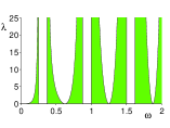
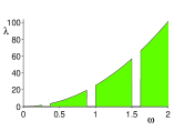
Figure 2: Lyapunov exponent versus frequency for quarter stack layered medium, for the “plus correlations” (left) and “minus correlations” (right), see Eqs. (11) and (9). Here $(Z_{a}+Z_{b})^{2}/Z_{a}Z_{b}=2.4$, $\mathcal{Z}\langle\varrho^{2}_{a}(n)\rangle(\pi n_{a}/c)^{2}=3.2$, $\mathcal{K}_{a}=1$.

Metamaterials. A special interest is in the mixed system in which the $a$-layer is a conventional right-handed (RH) material and $b$-layer is a left-handed (LH) material. This means that $\varepsilon_{a},\mu_{a},n_{a}>0$, whereas $\varepsilon_{b},\mu_{b},n_{b}<0$. However, both impedances remain positive, $Z_{a},Z_{b}>0$. Remarkably, in comparison with the conventional stack-structure, the expression (8) for the LE in this case stays the same. The only difference is that in the dispersion equation (5) the sign “plus” has to substitute for “minus” at the second term (the phase $\varphi_{b}\equiv k_{b}b=-\omega|n_{b}|b/c$). Such a “minor” correction can drastically change the frequency dependence of LE, see Fig. 1. Nevertheless, the LE caused by positional disorder, typically obeys the conventional dependence, $\lambda\propto\omega^{2}$ when $\omega\to 0$.

Note also that the ideal mixed stack ($\varepsilon_{a}=\mu_{a}=n_{a}=1$, $\varepsilon_{b}=\mu_{b}=n_{b}=-1$, $Z_{a}=Z_{b}=1$) has perfect transmission, $\lambda=0$, independently of a positional disorder.

One of the interesting features of the mixed layered structures is that for the RH-LH quarter stack ($n_{a}a=|n_{b}|b$) the average refractive index vanishes, $\overline{n}=(n_{a}a-|n_{b}|b)/(a+b)=0$. As a consequence, it follows from Eq. (5) that the spectral bands disappear and therefore, the transmission is absent, apart from a discrete set of frequencies where $k_{a}a=s\pi$ and $\gamma=0$ ($s=0,1,2,\ldots$). Evidently Eq. (8) is not valid in such a situation and an additional analysis has to be done.

It is important that in reality there is a frequency dependence of the permittivity $\varepsilon_{b}(\omega)$ and permeability $\mu_{b}(\omega)$ MS08 . This fact is crucial in applications. In particular, it leads to the following peculiarities. First, the mismatching factor $\varpi$ in Eq. (8) can vanish for specific values of frequency $\omega$ only, thus resulting in a resonance-like dependence for the transmission. Second, for typical frequency dependencies the refractive index of $b$-slabs takes an imaginary value giving rise to the emergence of new gaps. Specifically, such a gap can arise at the origin of spectrum, $\omega=0$, in contrast to conventional photonic crystals. It can be seen that in many aspects the wave transport through the bi-layered metamaterials is resembling to that of the electrons through double-barrier structures.

Electrons. The developed approach can be also applied to the propagation of electrons through the bi-layer structures with alternating potential barriers of the amplitudes $U_{a}$ and $U_{b}$ and slightly perturbed widths. Indeed, the stationary 1D Schrödinger equation for an electron with effective masses $m_{a}$, $m_{b}$ inside the barriers and total energy $E$ can be written in the form of Eq. (1), in which the partial wave numbers are associated with the barriers, $k_{a}=\sqrt{2m_{a}(E-U_{a})}/\hbar$ and $k_{b}=\sqrt{2m_{b}(E-U_{b})}/\hbar$. Another change, $\mu_{a,b}\to m_{a,b}$, should be done in the boundary condition on hetero-interfaces, $m_{a}^{-1}\psi^{\prime}_{a}(z_{i})=m_{b}^{-1}\psi^{\prime}_{b}(z_{i})$. Correspondingly, $Z_{b}/Z_{a}=k_{a}m_{b}/k_{b}m_{a}$ in the dispersion relation (5) and in the expression (8) for the LE.

If the energy $E$ is smaller then the heights of both barriers, $E<U_{a},\,U_{b}$, the electron wave numbers are purely imaginary. As a consequence, the electron states are strongly localized and the structure is non-transparent.

For other case when $U_{a}<E<U_{b}$, the tunneling propagation of electrons emerges. In this case the wave number $k_{a}$ is real while $k_{b}$ is imaginary. Therefore, the electron moves freely within any $a$-barrier and tunnels through the $b$-barriers. Thus, the expressions (8) for $\lambda$ and (5) for $\gamma$ have to be modified according to the change, $k_{b}\to i|k_{b}|$ and $\sin(k_{b}b)\to i\sinh(|k_{b}|b)$. As a result, the Fabry-Perot resonance increase of the LL arises only due to the second and third terms of Eq. (8). The general expression for the LE can be essentially simplified for a particular case of an array with delta-like potential barriers and slightly disordered distance between them. The corresponding expression for the LE is in full correspondence with that obtained in Ref. IKU01 .

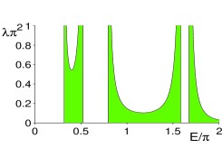
Figure 3: Lyapunov exponent vs. energy for electrons in bi-layered structure. Here $2m_{a}/\hbar^{2}=2m_{b}/\hbar^{2}=1$, $U_{a}=0.15$, $U_{b}=1.6$, $a=0.35\pi$, $b=0.65\pi$, $\langle\varrho^{2}_{a}(n)\rangle=(0.1a)^{2}$, $\langle\varrho^{2}_{b}(n)\rangle=(0.2b)^{2}$ The transition between tunneling and over-barrier scattering occurs at $E/\pi=0.5$.

For the over-barrier scattering, when $U_{a}<U_{b}<E$, both wave numbers, $k_{a}$ and $k_{b}$, are positive and the electron transport is similar to that for the conventional photonic stack but with dispersive parameters. The example of the energy dependence of the LE is given in Fig.3. It is interesting that if $E=(U_{b}m_{a}-U_{a}m_{b})/(m_{a}-m_{b})$, an electron does not change its velocity in the barriers, $\hbar k_{a}/m_{a}=\hbar k_{b}/m_{b}$, although its momentum changes, $\hbar k_{a}>\hbar k_{b}$. The LE vanishes in this case. Thus, such a “free” electron motion is equivalent to that in a homogeneous medium with perfect transmission.

Conclusion. We derived the expression for the inverse localization length for quasi-periodic bi-layer structures, whose widths are weakly perturbed. Our result can be applied both to conventional photonic crystals and to metamaterials, as well as to the electron superlattices. Another feature of the approach is that it takes into account possible correlations in a disorder that can lead to anomalous frequency (energy) dependence of transport properties. Due to the correlations one can significantly enhance or suppress the transmission/reflection through the bi-layered devices within the prescribed windows of frequency (energy) of electromagnetic (electron) waves. Our results may have a strong impact for the fabrication of a new class of disordered optic crystals, left/right handed metamaterials, and electron nanodevices with selective transmission and/or reflection.

F.M.I. acknowledges partial support by the VIEP BUAP-2008 grant.

References

- (1) P. Markoš and C. M. Soukoulis, Wave Propagation. From Electrons to Photonic Crystals and Left-Handed Materials (Princeton: Princeton University Press, 2008).
- (2) A. R. McGurn, K. T. Christensen, F. M. Mueller, and A. A. Maradudin, Phys. Rev. B47, 13120 (1993).
- (3) D. R. Smith et al., Phys. Rev. Lett. 84, 4184 (2000).
- (4) R. A. Shelby, D. R. Smith, and S. Schultz, Science 292, 77 (2001).
- (5) C. G. Parazzoli et al., Phys. Rev. Lett. 90, 107401 (2003).
- (6) A. Esmailpour, et al., Phys. Rev. B74, 024206 (2006).
- (7) D. Nau et al., Phys. Rev. Lett. 98, 133902 (2007).
- (8) I. V. Ponomarev et al., Phys. Rev. B75, 205434 (2007).
- (9) A. A. Asatryan et al., Phys. Rev. Lett. 99, 193902 (2007).
- (10) I. M. Lifshits, S. A. Gredeskul and L. A. Pastur, Introduction to the Theory of Disordered Systems ( New York: Wiley, 1988).
- (11) F. M. Izrailev and A. A. Krokhin, Phys. Rev. Lett. 82, 4062 (1999).
- (12) F. M. Izrailev, A. A. Krokhin, S. E. Ulloa, Phys. Rev. B63, 041102(R) (2001).
- (13) J. C. Hernández-Herrejón, F. M. Izrailev, and L. Tessieri, Physica E 40, 3137 (2008).
- (14) F. M. Izrailev and N. M. Makarov, Opt. Lett. 26, 1604 (2001); Appl. Phys. Lett. 84, 5150 (2004); J. Phys. A: Math. Gen. 38, 10613 (2005).
- (15) V. Bellani et al., Phys. Rev. Lett. 82, 2159 (1999).
- (16) U. Kuhl, F. M. Izrailev, A. A. Krokhin, H.-J. Stöckmann, Appl. Phys. Lett. 77, 633 (2000); U. Kuhl, F. M. Izrailev, and A. A. Krokhin, Phys. Rev. Lett. 100, 126402 (2008).
- (17) F. M. Izrailev, T. Kottos, and G. Tsironis, Phys. Rev. B 52 3274 (1995).
- (18) V. Baluni and J. Willemsen, Phys. Rev. A31, 3358 (1985).
- (19) E. Diez, F. M. Izrailev, A. A. Krokhin, and A. Rodriguez, Phys. Rev. B 78, 035118 (2008).