Splitting and composition methods in the numerical integration of differential equations

Abstract

We provide a comprehensive survey of splitting and composition methods for the numerical integration of ordinary differential equations (ODEs). Splitting methods constitute an appropriate choice when the vector field associated with the ODE can be decomposed into several pieces and each of them is integrable. This class of integrators are explicit, simple to implement and preserve structural properties of the system. In consequence, they are specially useful in geometric numerical integration. In addition, the numerical solution obtained by splitting schemes can be seen as the exact solution to a perturbed system of ODEs possessing the same geometric properties as the original system. This backward error interpretation has direct implications for the qualitative behavior of the numerical solution as well as for the error propagation along time. Closely connected with splitting integrators are composition methods. We analyze the order conditions required by a method to achieve a given order and summarize the different families of schemes one can find in the literature. Finally, we illustrate the main features of splitting and composition methods on several numerical examples arising from applications.

¹Instituto de Matemática Multidisciplinar, Universidad Politécnica de Valencia, E-46022 Valencia, Spain.

²Departament de Matemàtiques, Universitat Jaume I, E-12071 Castellón, Spain.

³Konputazio Zientziak eta A.A. saila, Informatika Fakultatea, EHU/UPV, Donostia/San Sebastián, Spain.

1 Introduction by examples

The basic idea of splitting methods for the time integration of ordinary differential equations (ODEs) can be formulated as follows. Given the initial value problem

$$x^{\prime}=f(x),\qquad x_{0}=x(0)\in\mathbb{R}^{D}$$ (1)

with $f:\mathbb{R}^{D}\longrightarrow\mathbb{R}^{D}$ and solution $\varphi_{t}(x_{0})$, let us suppose that $f$ can be expressed as $f=\sum_{i=1}^{m}f^{[i]}$ for certain functions $f^{[i]}:\mathbb{R}^{D}\longrightarrow\mathbb{R}^{D}$, in such a way that the equations

$$x^{\prime}=f^{[i]}(x),\qquad x_{0}=x(0)\in\mathbb{R}^{D},\qquad i=1,\ldots,m$$ (2)

can be integrated exactly, with solutions $x(h)=\varphi_{h}^{[i]}(x_{0})$ at $t=h$, the time step. Then, by combining these solutions as

$$\chi_{h}=\varphi_{h}^{[m]}\circ\cdots\circ\varphi_{h}^{[2]}\circ\varphi_{h}^{[1]}$$ (3)

and expanding $\chi$ into Taylor series, one finds that $\chi_{h}(x_{0})=\varphi_{h}(x_{0})+\mathcal{O}(h^{2})$, so that $\chi_{h}$ provides a first-order approximation to the exact solution. As we will see, it is possible to get higher order approximations by introducing more maps with additional coefficients, $\varphi_{a_{ij}h}^{[i]}$, in the previous composition (3).

One thus may say that splitting methods involve three steps: (i) choosing the set of functions $f^{[i]}$ such that $f=\sum_{i}f^{[i]}$; (ii) solving either exactly or approximately each equation $x^{\prime}=f^{[i]}(x)$; and (iii) combining these solutions to construct an approximation for (1). One obvious requirement is that the equations $x^{\prime}=f^{[i]}(x)$ should be simpler to integrate than the original system.

Some of the advantages that splitting methods possess can be summarized as follows:

• They are usually simple to implement.

• They are, in general, explicit.

• Their storage requirements are quite modest. The algorithms are sequential and the solutions at intermediate stages are stored in the solution vectors. This property can be of great interest when they are applied to partial differential equations (PDEs) previously semidiscretized.

• There exist in the literature a large number of specific methods tailored for different structures.

• They preserve structural properties of the exact solution, thus conferring to the numerical scheme a qualitative superiority with respect to other standard integrators, especially when long time intervals are considered. Examples of these structural features are symplecticity, volume preservation, time-symmetry and conservation of first integrals. In this sense, splitting methods constitute an important class of geometric numerical integrators.

Let us give more details on this last item. Traditionally, the goal of numerical integration of ODEs consists in computing the solution to the initial value problem (1) at time $t_{N}=Nh$ with a global error $\|x_{N}-x(t_{N})\|$ smaller than a prescribed tolerance and as efficiently as possible. To do that one chooses the class of method (one-step, multistep, extrapolation, etc.), the order (fixed or adaptive) and the time step (constant or variable). In contrast, with a geometric numerical integrator one typically fix a (not necessarily small) time step and compute solutions for very long times for several initial conditions, in order to get an approximate phase portrait of the system. It turns out that, although the global error of each trajectory may be large, the phase portrait is in some sense close to that of the original system.

The aim of geometric numerical integration is thus to reproduce the qualitative features of the solution of the differential equation which is being discretised, in particular its geometric properties [17, 41]. The motivation for developing such structure-preserving algorithms arises independently in areas of research as diverse as celestial mechanics, molecular dynamics, control theory, particle accelerators physics, and numerical analysis [41, 44, 57, 58, 49]. Although diverse, the systems appearing in these areas have one important common feature. They all preserve some underlying geometric structure which influences the qualitative nature of the phenomena they produce. In the field of geometric numerical integration these properties are built into the numerical method, which gives the method an improved qualitative behaviour, but also allows for a significantly more accurate long-time integration than with general-purpose methods. In addition to the construction of new numerical algorithms, an important aspect of geometric integration is the explanation of the relationship between preservation of the geometric properties of the scheme and the observed favorable error propagation in long-time integration.

Before proceeding further, let us introduce at this point some splitting methods and illustrate them on simple examples.

Example 1: Symplectic Euler and leapfrog schemes.

Suppose we have a Hamiltonian system of the form $H(q,p)=T(p)+V(q)$, where $q\in\mathbb{R}^{d}$ are the canonical coordinates, $p\in\mathbb{R}^{d}$ are the conjugate momenta, $T$ represents the kinetic energy and $V$ is the potential energy. Then the equations of motion read [36]

$$q^{\prime}=T_{p}(p),\qquad p^{\prime}=-V_{q}(q),$$ (4)

where $T_{p}$ and $V_{q}$ denote the vectors of partial derivatives. Equations (4) can be formulated as (1) with $x=(q,p)^{T}$, $f(x)=(T_{p},-V_{q})^{T}=J\nabla H(x)$ and $D=2d$. Here $J$ denotes the $2d\times 2d$ canonical symplectic matrix

$$J=\left(\begin{array}[]{rr}0&I_{d}\\ -I_{d}&0\end{array}\right)$$

and $I_{d}$ stands for the $d$-dimensional identity matrix. In this case the exact flow $\varphi_{t}$ is symplectic [1]. The simple Euler method applied to this system provides the following first order approximation for a time step $h$:

$$\begin{array}[]{lcl}q_{n+1}&=&q_{n}+hT_{p}(p_{n})\\ p_{n+1}&=&p_{n}-hV_{q}(q_{n}).\end{array}$$ (5)

On the other hand, if we consider $H$ as the sum of two Hamiltonians, the first one depending only on $p$ and the second only on $q$, the corresponding Hamilton equations

$$\begin{array}[]{lcl}q^{\prime}&=&T_{p}(p)\\ p^{\prime}&=&0\end{array}\qquad\mbox{ and }\qquad\begin{array}[]{lcl}q^{\prime}&=&0\\ p^{\prime}&=&-V_{q}(q)\end{array}$$ (6)

with initial condition $(q_{0},p_{0})$ can be readily solved to yield

$$\varphi_{t}^{[T]}:\;\begin{array}[]{lcl}q(t)&=&q_{0}+t\,T_{p}(p_{0})\\ p(t)&=&p_{0}\end{array}\qquad\mbox{ and }\qquad\varphi_{t}^{[V]}:\;\begin{array}[]{lcl}q(t)&=&q_{0}\\ p(t)&=&p_{0}-t\,V_{q}(q_{0}),\end{array}$$ (7)

respectively. Composing the time $t=h$ flow $\varphi_{h}^{[V]}$ (from initial condition $(q_{n},p_{n})$) followed by $\varphi_{h}^{[T]}$, gives the scheme

$$\chi_{h}\equiv\varphi_{h}^{[T]}\circ\varphi_{h}^{[V]}:\;\begin{array}[]{lcl}p_{n+1}&=&p_{n}-h\,V_{q}(q_{n})\\ q_{n+1}&=&q_{n}+h\,T_{p}(p_{n+1}).\end{array}$$ (8)

Since it is a composition of the flows of two Hamiltonian systems and in addition the composition of symplectic maps is again symplectic, $\chi_{h}$ is a symplectic integrator, which can be called appropriately the symplectic Euler method. It is of course also possible to compose the maps in the opposite order, $\varphi_{h}^{[V]}\circ\varphi_{h}^{[T]}$, thus obtaining another first order symplectic Euler scheme:

$$\chi_{h}^{*}\equiv\varphi_{h}^{[V]}\circ\varphi_{h}^{[T]}:\;\begin{array}[]{lcl}q_{n+1}&=&q_{n}+h\,T_{p}(p_{n})\\ p_{n+1}&=&p_{n}-h\,V_{q}(q_{n+1}).\end{array}$$ (9)

One says that (9) is the adjoint of $\chi_{h}$. Yet another possibility consists in using a ‘symmetric’ version

$$\mathcal{S}_{h}^{[2]}\equiv\varphi_{h/2}^{[V]}\circ\varphi_{h}^{[T]}\circ\varphi_{h/2}^{[V]},$$ (10)

which is known as the Strang splitting [77], the leapfrog or the Störmer–Verlet method [85], depending on the context where it is used. Observe that $\mathcal{S}_{h}^{[2]}=\chi_{h/2}\circ\chi_{h/2}^{*}$ and it is also symplectic and second order.

Example 2: Harmonic oscillator.

Let us consider now the Hamiltonian function $H(q,p)=\frac{1}{2}(p^{2}+q^{2})$, where now $q,p\in\mathbb{R}$. Then the corresponding equations (4) are linear and can be written as

$$x^{\prime}\equiv\left(\begin{array}[]{c}q^{\prime}\\ p^{\prime}\end{array}\right)=\Big{[}\underbrace{\left(\begin{array}[]{cc}0&1\\ 0&0\end{array}\right)}_{A}+\underbrace{\left(\begin{array}[]{cc}0&0\\ -1&0\end{array}\right)}_{B}\Big{]}\left(\begin{array}[]{c}q\\ p\end{array}\right)=(A+B)\,x.$$ (11)

This system has periodic solutions for which the energy $H$ is conserved. In addition, it is area preserving and time reversible. The numerical solution obtained by the Euler scheme (5) reads

$$\left(\begin{array}[]{c}q_{n+1}\\ p_{n+1}\end{array}\right)=\left(\begin{array}[]{cc}1&h\\ -h&1\end{array}\right)\,\left(\begin{array}[]{c}q_{n}\\ p_{n}\end{array}\right),$$ (12)

whereas the symplectic Euler method (9) leads to

$$\left(\begin{array}[]{c}q_{n+1}\\ p_{n+1}\end{array}\right)=\left(\begin{array}[]{cc}1&h\\ -h&1-h^{2}\end{array}\right)\,\left(\begin{array}[]{c}q_{n}\\ p_{n}\end{array}\right)={\rm e}^{hB}{\rm e}^{hA}\left(\begin{array}[]{c}q_{n}\\ p_{n}\end{array}\right).$$ (13)

Both render first order approximations to the exact solution, which can be expressed as $x(t)={\rm e}^{h(A+B)}x_{0}$, but there are important differences between them. First, the map (13) is area preserving (because it is symplectic), in contrast with (12). Second, the approximation obtained by the symplectic Euler scheme verifies

$$\frac{1}{2}(p_{n+1}^{2}+hp_{n+1}q_{n+1}+q_{n+1}^{2})=\frac{1}{2}(p_{n}^{2}+hp_{n}q_{n}+q_{n}^{2}).$$

Third, it can be shown that (13) is the exact solution at $t=h$ of the perturbed Hamiltonian system

$$\tilde{H}(q,p,h) = \frac{2\arcsin(h/2)}{h\sqrt{4-h^{2}}}(p^{2}+h\,p\,q+q^{2})$$

$$= \frac{1}{2}(p^{2}+q^{2})+h\,\left(\frac{1}{2}\,p\,q+\frac{1}{12}h(p^{2}+q^{2})+\cdots\right).$$

In other words, the numerical approximation (13), which is only of first order for the exact trajectories of the Hamiltonian $H(q,p)=\frac{1}{2}(p^{2}+q^{2})$, is in fact the exact solution of the perturbed Hamiltonian (1).

How these features manifest in actual simulations? To illustrate this point we take initial conditions $(q_{0},p_{0})=(4,0)$ and integrate with a time step $h=0.1$. Figure 1 shows the first five numerical approximations obtained by the Euler method (12) and the symplectic Euler scheme (13) in the left panel, and the results for the first 100 steps in the right panel. It is clear that for one time step there are not significant differences between the standard Euler and the symplectic Euler methods, but the picture is completely different for longer integrations, where the superiority of the splitting symplectic method is evident. Note that the numerical solution it provides evolves on a slightly perturbed ellipse.

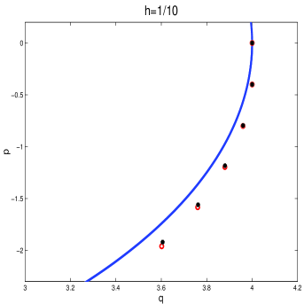
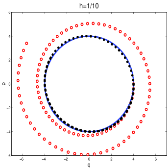
Figure 1: Numerical integration of the harmonic oscillator using the Euler method (white circles) and the symplectic Euler method (black circles) with initial condition $(q_{0},p_{0})=(4,0)$ and time step $h=\frac{1}{10}$. The left panel shows the results for the first 5 steps, whereas the right panel shows the results for the first 100 steps. The exact solution corresponds to the solid line.

Example 3: The 2-body problem (Kepler problem).

The motion of two bodies attracting each other through the gravitational law can be described by

$$q_{i}^{\prime\prime}=-\frac{q_{i}}{(q_{1}^{2}+q_{2}^{2})^{3/2}},\qquad i=1,2$$ (15)

in conveniently normalized coordinates in the plane of motion. This system has a number of characteristic geometric properties. First, equations (15) can be derived from the Hamiltonian function

$$H(q,p)=T(p)+V(q)=\frac{1}{2}(p_{1}^{2}+p_{2}^{2})-\frac{1}{r},\qquad r=\sqrt{q_{1}^{2}+q_{2}^{2}}.$$ (16)

Second, it is invariant under continuous translations in time and rotations in space, and thus both the Hamiltonian and the angular momentum $L=q_{1}p_{2}-q_{2}p_{1}$ are preserved. In addition, the so-called Laplace–Runge–Lenz vector is also constant along their solutions, due to the fact that the symmetry group of this problem is the group of four-dimensional real proper rotations $\mathrm{SO}(4)$ [36].

For the numerical integration of this problem we choose as initial value

$$q_{1}(0)=1-e,\quad q_{2}(0)=0,\quad p_{1}(0)=0,\quad p_{2}(0)=\sqrt{\frac{1+e}{1-e}},$$ (17)

where $0\leq e<1$ represents the eccentricity of the orbit. In this case the total energy is $H=H_{0}=-1/2$, the period of the solution is $2\pi$, the initial condition corresponds to the pericenter and the major semiaxis of the ellipse is 1.

Figure 2 shows some numerical solutions obtained with schemes (5) and (8) for the initial conditions (17) with eccentricity $e=0.6$. The left panel shows the results for the integration of 3 periods with time step $h=\frac{1}{100}$. As in the previous example, the explicit Euler method provides an approximate orbit that spirals outwards, whereas the symplectic Euler scheme merely distorts the ellipse, but also exhibits a precession effect. To better illustrate this effect, we repeat the experiment for a longer interval (15 periods) and a larger time step ($h=\frac{1}{20}$) in the right panel. The explanation of these phenomena can be formulated as follows. On the one hand, the symplectic Euler method exactly conserves the angular momentum. On the other hand, the numerical solution it provides can be seen as the exact solution of a slightly perturbed Kepler problem, and thus $\mathrm{SO}(4)$ is no longer the symmetry group of the problem, so that the Laplace–Runge–Lenz vector is not preserved and the trajectories are not closed anymore.

,

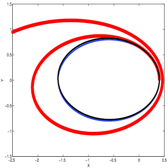
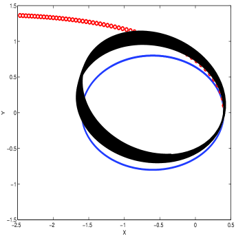
Figure 2: Numerical integration of the 2-body problem using the Euler method (white circles) and the symplectic Euper scheme (black circles) for the initial conditions (17) with eccentricity $e=0.6$. The left panel shows the results for $h=\frac{1}{100}$ and the first 3 periods and the right panel shows the results for $h=\frac{1}{20}$ and the first 15 periods.

Next we check how the error in the preservation of energy and the global error in position propagates with time. For comparison, we also include the results obtained with a Runge–Kutta method of order 2 (Heun’s method) and the leapfrog scheme (10). We now consider $e=1/5$ and integrate for 500 periods. The step size is $h=\frac{2\pi}{1500}$ in all cases, except for the Heun method which uses $h=\frac{2\pi}{750}$ instead. In this way all methods require the same number of force evaluations (Heun’s method computes twice the force per step). The corresponding results are shown in Figure 3 in a log-log scale. Notice that the average error in energy does not grow for the split symplectic methods and the error in positions grows only linearly with time, in contrast with Euler and Heun schemes. The Störmer–Verlet integrator provides more accurate results than the Heun method with the same computational cost.

,

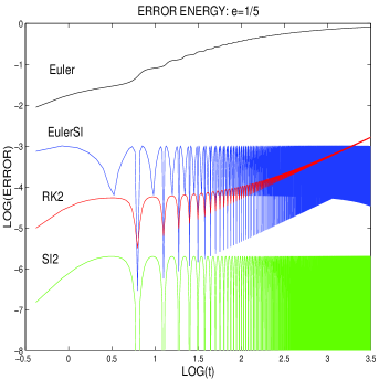
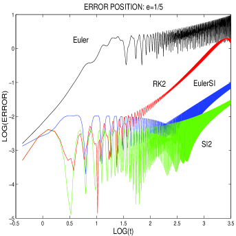
Figure 3: Error growth in energy and position for the Kepler problem with $e=1/5$ and 500 periods achieved by the first order symplectic Euler (EulerSI) and the second order Störmer–Verlet integrator (SI2). For comparison, we also include the first order Euler and the second order Heun (RK2) methods. The time step is adjusted in such a way that all methods use 1500 force evaluations per period.

A collection of (additional) examples.

Splitting methods constitute an important tool in different areas of science. In addition to Hamiltonian systems, they can be successfully applied in the numerical study of Poisson systems, systems possessing integrals of the motion (such as energy and angular momentum) and systems with (continuous, discrete and time-reversal) symmetries. As a matter of fact, splitting methods have been designed (often independently) and extensively used in fields as distant as molecular dynamics, simulation of storage rings in particle accelerators, celestial mechanics and quantum physics simulations. To see why this is so, next we collect a number of differential equations which appear in different contexts ranging from Celestial Mechanics to electromagnetism and Quantum Mechanics. These examples also try to illustrate the fact that very often one particular equation can be split into different ways and the most appropriate methods may depend on the split chosen.

We (arbitrarily) classify our examples into three different categories.

1. Hamiltonian systems.

   (a)

   Generalized harmonic oscillator ($M,N\in\mathbb{R}^{d\times d}$):

   $$H=\frac{1}{2}p^{T}Mp+\frac{1}{2}q^{T}Nq.$$ (18)

   (b)

   Hénon–Heiles Hamiltonian [43]:

   $$H=\frac{1}{2}(p_{1}^{2}+p_{2}^{2})+\frac{1}{2}(q_{1}^{2}+q_{2}^{2})+q_{1}^{2}q_{2}-\frac{1}{3}q_{2}^{3}.$$ (19)

   (c)

   Perturbed Kepler problem. It models the dynamics of a satellite moving into the gravitational field produced by a slightly oblate planet:

   $$H=\frac{1}{2}(p_{1}^{2}+p_{2}^{2})-\frac{1}{r}-\frac{\varepsilon}{2r^{3}}\left(1-\frac{3q_{1}^{2}}{r^{2}}\right)$$ (20)

   where $\varepsilon$ is typically a small parameter. When $\varepsilon=0$, the 2-body problem (16) is recovered.

   (d)

   The gravitational $N$-body problem ($q_{i},p_{i}\in\mathbb{R}^{3},\ i=1,\ldots,N$):

   $$H=\frac{1}{2}\sum_{i=1}^{N}\frac{1}{2m_{i}}p_{i}^{T}p_{i}-G\sum_{i=2}^{N}\sum_{j=1}^{i-1}\frac{m_{i}m_{j}}{\|q_{i}-q_{j}\|}.$$ (21)

   (e)

   The motion of a charged particle in a constant magnetic field perturbed by $k$ electrostatic plane waves [21]:

   $$H(q,p,t)=\frac{1}{2}p^{2}+\frac{1}{2}q^{2}+\varepsilon\sum_{i=1}^{k}\cos(q-\omega_{i}t).$$ (22)

2. More general dynamical systems.

   (a)

   The Volterra–Lotka problem [41],

   $$\frac{d}{dt}\left[\begin{array}[]{c}u\\ v\end{array}\right]=\left[\begin{array}[]{rr}-2&0\\ 0&1\end{array}\right]\left[\begin{array}[]{c}u\\ v\end{array}\right]+\left[\begin{array}[]{r}uv\\ -uv\end{array}\right]=\left[\begin{array}[]{c}u(v-2)\\ 0\end{array}\right]+\left[\begin{array}[]{c}0\\ v(1-u)\end{array}\right],$$ (23)

   with first integral $I(u,v)=\log u-u+2\log v-v$.

   (b)

   The Lorenz system [52, 39] (split into linear and non-linear parts):

   $$\frac{d}{dt}\left[\begin{array}[]{c}x\\ y\\ z\end{array}\right]=\left[\begin{array}[]{rrr}-\sigma&\sigma&0\\ r&-1&0\\ 0&0&b\end{array}\right]\left[\begin{array}[]{c}x\\ y\\ z\end{array}\right]+\left[\begin{array}[]{rrr}0&0&0\\ 0&0&-x\\ 0&x&0\end{array}\right]\left[\begin{array}[]{c}x\\ y\\ z\end{array}\right].$$ (24)

   Here $\sigma,r,b>0$ are constant. The values considered in [52] were $\sigma=10$, $r=28$ and $b=8/3$.

   (c)

   The ABC-flow ($f=f_{A}+f_{B}+f_{C}$, but other splits are also possible [57]):

   $$\frac{d}{dt}(x,y,z)=A(0,\sin x,\cos x)+B(\cos y,0,\sin y)+C(\sin z,\cos z,0).$$ (25)

3. Evolutionary PDEs.

   Although we are mainly concerned here with splitting methods applied to ODEs, it turns out that they can also be used in the numerical integration of certain partial differential equations. Specifically, a number of PDEs relevant in the applications, after an appropriate space discretization, lead to a system of ODEs which can be subsequently solved numerically by splitting methods. Among these equations, the following are worth to be mentioned.

   (a)

   The Schrödinger equation ($\hbar=1$):

   $$i\frac{\partial}{\partial t}\Psi(x,t)=\left(-\frac{1}{2m}\nabla^{2}+V(x)\right)\Psi(x,t).$$ (26)

   (b)

   The Gross–Pitaevskii equation [68]:

   $$i\frac{\partial}{\partial t}\Psi(x,t)=\left(-\frac{1}{2m}\nabla^{2}+V(x)+\alpha|\Psi(x,t)|^{2}\right)\Psi(x,t)$$ (27)

   (c)

   The Maxwell equations

   $$\frac{\partial}{\partial t}{\bf B}=-\frac{1}{\mu}{\bf\nabla\times E},\qquad\frac{\partial}{\partial t}{\bf E}=\frac{1}{\varepsilon}{\bf\nabla\times B},$$ (28)

   where ${\bf E}(x,t)$, ${\bf B}(x,t)$ are the electric and magnetic field vectors, $\mu(x)$ is the the permeability and $\varepsilon(x)$ is the permittivity.

As we stated before, splitting methods form a subclass of geometric numerical integrators for various types of ODEs. The reason is easy to grasp from the examples analyzed before. Suppose that the flow of the original differential equation (1) forms a particular group of diffeomorphisms (in the case of Hamiltonian system, the group of symplectic maps). If $f$ is conveniently split as $f=\sum_{i}f^{[i]}$ (step (i) in the construction process of a splitting scheme) and the flows corresponding to each $f^{[i]}$ also belong to the same group of diffeomorphisms in such a way that they can be explicitly obtained (step (ii)), then, by composing these flows (step (iii)) we get an approximation in the group, thus inheriting geometric properties of the exact solution. These considerations also hold (with some modifications) when the exact flow forms a semigroup or a symmetric space.

With respect to steps (i) and (ii) before, several comments are in order. First, whereas for certain classes of ODEs, the splitting can be constructed systematically for any $f$, in other cases no general procedure is known, and thus one has to proceed on a case by case basis. Second, sometimes a standard splitting is possible for a certain $f$, but there exist other possible choices leading to more efficient schemes (we will see some examples in section 8). Third, whereas the original system possesses several geometric properties which are interesting to preserve by the numerical scheme, different splittings preserve different properties and it is not always possible to find one splitting preserving all of them. These aspects have been analyzed in detail in [57], where a classification of ODEs and general guidelines to find suitable splittings in each case is provided. Here, by contrast, we will concentrate on the third step of any splitting method: given a particular splitting, we will show how to combine the flows of the pieces $f^{[i]}$ to get efficient higher order approximations. In any case, the reader is referred to the excellent review paper [57] and the monographs [41, 49], where these and other issues, mainly in connection with geometric numerical integration, are thoroughly examined.

2 Splitting and composition methods

2.1 Increasing the order of an integrator by composition

It is well known that numerical integrators of arbitrarily high order can be obtained by composition of a basic integrator of low order. Consider for instance the leapfrog scheme (10), which is a second-order integrator ${\mathcal{S}}^{[2]}:\mathbb{R}^{2d}\to\mathbb{R}^{2d}$. Then, a 4th order integrator ${\mathcal{S}}^{[4]}:\mathbb{R}^{2d}\to\mathbb{R}^{2d}$ can be obtained as

$${\mathcal{S}}_{h}^{[4]}={\mathcal{S}}_{\alpha h}^{[2]}\circ{\mathcal{S}}_{\beta h}^{[2]}\circ{\mathcal{S}}_{\alpha h}^{[2]},\quad\mbox{ with }\quad\alpha=\frac{1}{2-2^{1/3}},\qquad\beta=1-2\alpha.$$ (29)

More generally, if one recursively defines ${\mathcal{S}}^{[2k+2]}:\mathbb{R}^{2d}\to\mathbb{R}^{2d}$ for $k=1,2,\ldots$ as

$${\mathcal{S}}_{h}^{[2k+2]}={\mathcal{S}}_{\alpha h}^{[2k]}\circ{\mathcal{S}}_{\beta h}^{[2k]}\circ{\mathcal{S}}_{\alpha h}^{[2k]},$$ (30)

with

$$\alpha=\frac{1}{2-2^{1/(2k+1)}},\qquad\beta=1-2\alpha,$$ (31)

then the schemes ${\mathcal{S}}_{h}^{[2k]}$ are of order $2k$ ($k\geq 1$) [78, 88]. We will prove later on this assertion. At this point it is useful to introduce the notion of adjoint of a given integrator $\psi_{h}$ [73]. By definition, this is the method $\psi_{h}^{\ast}$ such that $\psi_{h}^{\ast}=\psi_{-h}^{-1}$. A method that is equal to its own adjoint is called self-adjoint or (time-)symmetric. In this case, $\psi_{-h}\circ\,\psi_{h}=\mathrm{id}$. Since the leapfrog scheme (10) can be rewritten as

$${\mathcal{S}}_{h}^{[2]}=\chi_{h/2}\circ\chi_{h/2}^{*},$$ (32)

where $\chi_{h}$ is the symplectic Euler method (8), then ${\mathcal{S}}_{h}^{[2]}$ is certainly time-symmetric. Actually, given any basic first order integrator $\chi_{h}:\mathbb{R}^{D}\to\mathbb{R}^{D}$ for the ODE system (1), the composition (32) is a time-symmetric method of order $2$, and the other way around: any self-adjoint second order integrator can be expressed as (32). Furthermore, the integrators ${\mathcal{S}}_{h}^{[2k]}$ ($k=1,2,\ldots$) recursively defined by (30)–(31) are time-symmetric methods of order $2k$. In particular, if $f(x)$ in the ODE (1) is split as

$$f(x)=\sum_{i=1}^{m}f^{[i]}(x)$$ (33)

then, time-symmetric integrators ${\mathcal{S}}_{h}^{[2k]}$ of order $2k$ can be constructed in this way by considering the basic first order integrator

$$\chi_{h}=\varphi_{h}^{[m]}\circ\cdots\circ\varphi_{h}^{[2]}\circ\varphi_{h}^{[1]}$$ (34)

and its adjoint

$$\chi^{*}_{h}=\chi_{-h}^{-1}=\varphi_{h}^{[1]}\circ\varphi_{h}^{[2]}\circ\cdots\circ\varphi_{h}^{[m]}.$$

This general procedure of constructing geometric integrators of arbitrarily high order, although simple, presents some drawbacks. In particular, the resulting methods require a large number of evaluations and usually have large truncation errors.

As we will show, efficient schemes can be built by considering more general composition integrators. First observe that the $(2k)$th order integrators ${\mathcal{S}}_{h}^{[2k]}$ can be rewritten in the form

$$\psi_{h}=\chi_{\alpha_{2s}h}\circ\chi^{*}_{\alpha_{2s-1}h}\circ\cdots\circ\chi_{\alpha_{2}h}\circ\chi^{*}_{\alpha_{1}h}$$ (35)

with $s=3^{k-1}$ and some fixed coefficients $(\alpha_{1},\ldots,\alpha_{2s})\in\mathbb{R}^{2s}$. Then the idea is to consider composition integrators of the form (35) with appropriately chosen coefficients $(\alpha_{1},\ldots,\alpha_{2s})\in\mathbb{R}^{2s}$.

In the particular case where the ODE (1) is split in two parts $f=f^{[a]}+f^{[b]}$ and $\chi_{h}=\varphi^{[b]}_{h}\circ\varphi^{[a]}_{h}$, one can trivially check that the composition integrator (35) can be rewritten as

$$\psi_{h}=\varphi^{[b]}_{b_{s+1}h}\circ\varphi^{[a]}_{a_{s}h}\circ\varphi^{[b]}_{b_{s}h}\circ\cdots\circ\varphi^{[b]}_{b_{2}h}\circ\varphi^{[a]}_{a_{1}h}\circ\varphi^{[b]}_{b_{1}h},$$ (36)

where $b_{1}=\alpha_{1}$ and for $j=1,\ldots,s$,

$$a_{j}=\alpha_{2j-1}+\alpha_{2j},\qquad\quad b_{j+1}=\alpha_{2j}+\alpha_{2j+1}$$ (37)

(with $\alpha_{2s+1}=0$). Conversely, any integrator of the form (36) satisfying that $\sum_{i=1}^{s}a_{i}=\sum_{i=1}^{s+1}b_{i}$ can be expressed in the form (35) with $\chi_{h}=\varphi^{[b]}_{h}\circ\varphi^{[a]}_{h}$. For later reference, we state the following result, due to McLachlan [54].

Theorem 1

The integrator (36) is of order $r$ for ODEs of the form (1) with $f:\mathbb{R}^{D}\longrightarrow\mathbb{R}^{D}$ arbitrarily split as $f=f^{[a]}+f^{[b]}$ if and only if the integrator (35) (with coefficients $\alpha_{j}$ obtained from (37)) is of order $r$ for arbitrary consistent integrators $\chi_{h}$.

2.2 Integrators and series of differential operators

Before proceeding further with the analysis, let us relate generic numerical integrators with formal series of differential equations. This relationship will allow one to formulate in a rather simple way the conditions to be satisfied by an integration scheme to achieve a given order of consistency.

First of all, let us recall that an integrator $\psi_{h}:\mathbb{R}^{D}\to\mathbb{R}^{D}$ for the system (1) is said to be of order $r$ if for all $x\in\mathbb{R}^{D}$

$$\psi_{h}(x)=\varphi_{h}(x)+{\mathcal{O}}(h^{r+1})$$ (38)

as $h\rightarrow 0$, where $\varphi_{h}$ is the $h$-flow of the ODE (1).

It is well known that, for any smooth function $g:\mathbb{R}^{D}\rightarrow\mathbb{R}$, it formally holds that [66]

$$g(\varphi_{h}(x))=g(x)+\sum_{n\geq 1}\frac{1}{n!}F^{n}[g](x)=\exp(hF)[g](x),$$

where $F$ is the Lie derivative associated to the ODE system (1), i.e., the first order linear differential operator $F$ acting on functions in $C^{\infty}(\mathbb{R}^{D},\mathbb{R})$ as follows. For each $g\in C^{\infty}(\mathbb{R}^{D},\mathbb{R})$ and each $x=(x_{1},\ldots,x_{D})\in\mathbb{R}^{D}$

$$F[g](x)=\sum_{j=1}^{D}f_{j}(x)\frac{\partial g}{\partial x_{j}}(x),$$ (39)

where $f(x)=(f_{1}(x),\ldots,f_{D}(x))^{T}$. Motivated by this fact, we consider for a basic integrator $\chi_{h}:\mathbb{R}^{D}\to\mathbb{R}^{D}$, the linear differential operators $X_{n}$ ($n\geq 1$) acting on smooth functions $g\in C^{\infty}(\mathbb{R}^{D},\mathbb{R})$ as follows:

$$X_{n}[g](x)=\frac{1}{n!}\frac{d^{n}}{dh^{n}}\left.g(\chi_{h}(x))\right|_{h=0},$$ (40)

so that formally $g(\chi_{h}(x))=X(h)[g](x)$, where

$$X(h)=I+\sum_{n\geq 1}h^{n}X_{n},$$ (41)

and $I$ denotes the identity operator. Thus, the integrator $\chi_{h}$ is of order $r$ if

$$X_{n}=\frac{1}{n!}F^{n},\qquad 1\leq n\leq r.$$

Alternatively, one can consider the series of vector fields

$$Y(h)=\sum_{n\geq 1}h^{n}Y_{n}=\log(X(h))=\sum_{m\geq 1}\frac{(-1)^{m+1}}{m}\left(hX_{1}+h^{2}X_{2}+\cdots\right)^{m},$$

that is,

$$Y_{n}=\sum_{m\geq 1}^{n}\frac{(-1)^{m+1}}{m}\sum_{j_{1}+\cdots+j_{m}=n}X_{j_{1}}\cdots X_{j_{m}},$$

so that $X(h)=\exp(Y(h))$, and formally, $g(\chi_{h}(x))=\exp(Y(h))[g](x)$. Clearly, the basic integrator is of order $r$ if

$$Y_{1}=F,\qquad Y_{n}=0\quad\mbox{for}\quad 2\leq n\leq r.$$

For the adjoint integrator $\chi^{*}_{h}=\chi_{-h}^{-1}$, one obviously gets $g(\chi^{*}_{h}(x))={\rm e}^{-Y(-h)}[g](x)$. This shows that $\chi_{h}$ is time-symmetric if and only if $Y(h)=hY_{1}+h^{3}Y_{3}+\cdots$, and in particular, that time-symmetric methods are of even order.

It is possible now to check that the symmetric integrators ${\mathcal{S}}_{h}^{[2k]}$ given by (30)–(31) are actually schemes of order $2k$ provided that ${\mathcal{S}}_{h}^{[2]}$ is a symmetric second order integrator. Consider the series of differential operators

$$F^{[2k]}(h)=hF+h^{2k+1}F_{2k+1}^{[2k]}+h^{2k+3}F_{2k+3}^{[2k]}+\cdots$$

such that $g({\mathcal{S}}_{h}^{[2k]}(x))=\exp(F^{[2k]}(h))[g](x)$. Then one clearly has

$$\exp(F^{[2k+2]}(h))=\exp(F^{[2k]}(\alpha h))\exp(F^{[2k]}(\beta h))\exp(F^{[2k]}(\alpha h))$$

which implies

$$F^{[2k+2]}(h)=h\,(2\alpha+\beta)\,F+h^{2k+1}\,(2\alpha^{2k+1}+\beta^{2k+1})\,F_{2k+1}^{[2k]}+\mathcal{O}(h^{2k+3}),$$

and thus ${\mathcal{S}}_{h}^{2k+2}$ is of order $2k+2$ provided that ${\mathcal{S}}_{h}^{2k}$ is of order $2k$ and $\alpha$ and $\beta$ satisfy the equations

$$2\alpha+\beta=1,\qquad 2\alpha^{2k+1}+\beta^{2k+1}=0,$$

whose unique real solution is given by (31).

In the general case, for the composition method (35) we have

$$g(\psi_{h}(x))=\Psi(h)[g](x),$$

where $\Psi(h)=I+h\Psi_{1}+h^{2}\Psi_{2}+\cdots$ is a series of differential operators satisfying

$$\Psi(h)=X(-\alpha_{1}h)^{-1}X(\alpha_{2}h)\cdots X(-\alpha_{2s-1}h)^{-1}X(\alpha_{2s}h),$$ (42)

where the series $X(h)$ is given by (40)–(41), and

$$X(h)^{-1}=I+\sum_{m\geq 1}(-1)^{m+1}\left(hX_{1}+h^{2}X_{2}+\cdots\right)^{m}.$$ (43)

Thus, the order of a composition integrator of the form (35) can be checked by comparing the series of differential operators $\Psi(h)$ with the series $\exp(hF)$ associated to the flow of the system (1). That is, the integrator (35) is of order $r$ if

$$\Psi_{n}=\frac{1}{n!}F^{n},\qquad 1\leq n\leq r.$$ (44)

Instead of using (42) to obtain the terms $\Psi_{n}$ of the series $\Psi(h)$, one can equivalently consider the formal equality

$$\Psi(h)={\rm e}^{-Y(-h\alpha_{1})}\,{\rm e}^{Y(h\alpha_{2})}\cdots\,{\rm e}^{-Y(-h\alpha_{2s-1})}\,{\rm e}^{Y(h\alpha_{2s})},$$ (45)

to obtain the series expansion of $\log(\Psi(h))=\sum_{n\geq 1}h^{n}F_{n}$, so that $r$th order compositions methods can also be characterized by the conditions

$$F_{1}=F,\qquad F_{n}=0\quad\mbox{for}\quad 2\leq n\leq r.$$ (46)

As for the splitting integrator (36) when the ODE (1) is split in two parts,

$$f(x)=f^{[a]}(x)+f^{[b]}(x),$$ (47)

let $F^{[a]}$ and $F^{[b]}$ be the Lie derivatives corresponding to $f^{[a]}$ and $f^{[b]}$ respectively, that is,

$$F^{[a]}[g](x)=\sum_{j=1}^{D}f_{j}^{[a]}(x)\frac{\partial g}{\partial x_{j}}(x),\qquad F^{[b]}[g](x)=\sum_{j=1}^{D}f_{j}^{[b]}(x)\frac{\partial g}{\partial x_{j}}(x)$$ (48)

for each $g\in C^{\infty}(\mathbb{R}^{D},\mathbb{R})$ and each $x\in\mathbb{R}^{D}$. Then, the series $\Psi(h)$ of differential operators associated to the integrator $\psi_{h}$ in (36) can be formally written as

$$\Psi(h)={\rm e}^{b_{1}hF^{[b]}}\,{\rm e}^{a_{1}hF^{[a]}}\cdots\,{\rm e}^{b_{s}hF^{[b]}}\,{\rm e}^{a_{s}hF^{[a]}}\,{\rm e}^{b_{s+1}hF^{[b]}}.$$ (49)

3 Order conditions of splitting and composition methods

There are several procedures to get the order conditions for the coefficients of splitting and composition methods of a given order. These are, generally speaking, large systems of polynomial equations in the coefficients which are obtained from equations (46). Perhaps the two most popular are (i) the expansion of the series $\log(\Psi(h))=\sum_{n\geq 1}h^{n}F_{n}$ of vector fields by applying recursively the Baker–Campbell–Hausdorff (BCH) formula [88], and (ii) a generalization of the theory of rooted trees used in the theory of Runge–Kutta methods, which allows one to get an equivalent set of simpler order conditions in a systematic way [63] (see also [41]). In this section we first summarize briefly how to get these equations with the BCH formula, and then we present a novel approach, related to that in [63], but based on Lyndon words instead of rooted trees.

3.1 Order conditions via BCH formula

As is well known, if $X$ and $Y$ are two non-commuting operators, the BCH formula establishes that formally, ${\rm e}^{X}{\rm e}^{Y}={\rm e}^{Z}$, where $Z$ belongs to the Lie algebra ${\mathcal{L}}(X,Y)$ generated by $X$ and $Y$ with the commutator $[X,Y]=XY-YX$ as Lie bracket [84]. Moreover,

$$Z=\log({\rm e}^{X}\,{\rm e}^{Y})=X+Y+\sum_{m=2}^{\infty}\,Z_{m},$$ (50)

with $Z_{m}(X,Y)$ a homogeneous Lie polynomial in $X$ and $Y$ of degree $m$, i.e., it is a $\mathbb{Q}$-linear combination of commutators of the form $[V_{1},[V_{2},\ldots,[V_{m-1},V_{m}]\ldots]]$ with $V_{i}\in\{X,Y\}$ for $1\leq i\leq m$. The first terms read

$$Z_{2} = \frac{1}{2}[X,Y]$$

$$Z_{3} = -\frac{1}{12}[[X,Y],X]+\frac{1}{12}[[X,Y],Y]$$

$$Z_{4} = \frac{1}{24}[[[X,Y],Y],X],$$

and explicit expressions up to $m=20$ have been recently computed in an arbitrary generalized Hall basis of ${\mathcal{L}}(X,Y)$ [22].

The procedure to get the order conditions for the composition method (35) with this approach can be summarized as follows. First, consider the series of differential operators $\Psi(h)$ associated to the integrator (35), expressed as a product of exponentials of vector fields, i.e., equation (45). Then, apply repeatedly the BCH formula to get the series expansion $\log(\Psi(h))=\sum_{n\geq 1}h^{n}F_{n}$. In this way, one gets

$$\log(\Psi(h)) = hw_{1}Y_{1}+h^{2}w_{2}Y_{2}+h^{3}(w_{3}Y_{3}+w_{12}[Y_{1},Y_{2}])$$

$$+h^{4}(w_{4}Y_{4}+w_{13}[Y_{1},Y_{3}]+w_{112}[Y_{1},[Y_{1},Y_{2}]])+{\mathcal{O}}(h^{5})$$

where the $w_{j_{1}\cdots j_{m}}$ are polynomials of degree $n=j_{1}+\cdots+j_{m}$ in the parameters $\alpha_{1},\ldots,\alpha_{2s}$. The first such polynomials are

$$w_{1}=\sum_{i=1}^{2s}\alpha_{i},\qquad w_{2}=\sum_{i=1}^{2s}(-1)^{i}\alpha_{i}^{2},\qquad w_{3}=\sum_{i=1}^{2s}\alpha_{i}^{3}.$$ (52)

In general, the expressions of the polynomials $w_{j_{1}\cdots j_{m}}$ in (3.1) obtained by repeated application of the BCH formula are rather cumbersome.

The order conditions for the composition integrator (35) are then obtained by imposing equations (46) to guarantee that the scheme has order $r\geq 1$. Thus, the order conditions are $w_{1}=1$, and $w_{j_{1}\cdots j_{m}}=0$ whenever $2\leq j_{1}+\cdots+j_{m}\leq r$.

One can proceed similarly to get the order conditions of the splitting scheme (36) in terms of the coefficients $a_{i},b_{i}$: Consider the series of differential operators $\Psi(h)$ associated to the integrator (36) expressed as (49); then, apply repeatedly the BCH formula to get the series expansion $\log(\Psi(h))=\sum_{n\geq 1}h^{n}F_{n}$, so that the order conditions will be obtained by imposing equations (46) to guarantee order $r\geq 1$. It can be seen that the following holds for $\log(\Psi(h))$,

$$\log(\Psi(h)) = h(v_{a}F^{[a]}+v_{b}F^{[b]})+h^{2}v_{ab}F^{[ab]}+h^{3}(v_{abb}F^{[abb]}+v_{aba}F^{[aba]})$$ (53)

$$+h^{4}(v_{abbb}F^{[abbb]}+v_{abba}F^{[abba]}+v_{abaa}F^{[abaa]})+{\mathcal{O}}(h^{5}),$$

where

$$F^{[ab]} \!=\! [F^{[a]},F^{[b]}],\quad F^{[abb]}=[F^{[ab]},F^{[b]}],\quad F^{[aba]}=[F^{[ab]},F^{[a]}],$$

$$F^{[abbb]} \!=\! [F^{[abb]},F^{[b]}],\quad F^{[abba]}=[F^{[abb]},F^{[a]}],\quad F^{[abaa]}=[F^{[aba]},F^{[a]}],$$

and $v_{a},v_{b},v_{ab},v_{abb},v_{aba},v_{abbb},\ldots$ are polynomials in the parameters $a_{i},b_{i}$ of the splitting scheme (36). In particular, one gets

$$v_{a} \!=\! \sum_{i=1}^{s}a_{i},\qquad v_{b}=\sum_{i=1}^{s+1}b_{i},\qquad v_{ab}=\frac{1}{2}v_{a}v_{b}-\sum_{1\leq i\leq j\leq s}b_{i}a_{j},$$ (54)

$$2v_{aba} \!=\! -\frac{1}{6}v_{a}^{2}v_{b}+\sum_{1\leq i<j\leq k\leq s}a_{i}b_{j}a_{k},\qquad 2v_{abb}=\frac{1}{6}v_{a}v_{b}^{2}-\sum_{1\leq i\leq j<k\leq s+1}b_{i}a_{j}b_{k}.$$

From (53), we see that a characterization of the order of the splitting scheme (36) can be obtained by considering $v_{a}=v_{b}=1$ and $v_{ab}=v_{abb}=v_{aba}=\cdots=0$ up to polynomials of that form of the required order. The set of order conditions thus obtained will be independent in the general case if the vector fields $F^{[a]},F^{[b]},F^{[ab]},F^{[abb]},F^{[aba]}$ considered in (53) correspond to a basis of the free Lie algebra on the alphabet $\{a,b\}$. Notice that in (53) we have considered a Hall basis (the classical basis of P. Hall) associated to the Hall words $a,b,ab,abb,aba,abbb,abba,abaa,\cdots$ [69]. The coefficients $v_{w}$ in (53) corresponding to each Hall word $w$ can be systematically obtained using the results in [62] in terms of rooted trees and iterated integrals. An efficient algorithm (based on the results in [62]) of the BCH formula and related calculations that allows one to obtain (53) up to terms of arbitrarily high degree is presented in [22].

3.2 A set of independent order conditions

We next present a set of order conditions for composition integrators (35) derived in [25].

From (41)–(43), it follows that

$$\Psi(h)=I+\sum_{n\geq 1}h^{n}\sum_{j_{1}+\cdots+j_{r}=n}u_{j_{1}\cdots j_{r}}(\alpha_{1},\ldots,\alpha_{2s})\,X_{j_{1}}\cdots X_{j_{r}},$$ (55)

for some polynomial functions $u_{j_{1}\cdots j_{r}}$ of the parameters $\alpha_{1},\ldots,\alpha_{2s}$ of the method. We next introduce some notation in order to explicitly write these polynomials. For each positive integer $j$, we write $j^{*}=j-1$ if $j$ is even, and $j^{*}=j$ if $j$ is odd. Finally, for each pair $(i,j)$ of positive integers, we write $\alpha_{j}^{(i)}=(-1)^{j(i-1)}(\alpha_{j})^{i}$. That is, $\alpha_{j}^{(i)}=(\alpha_{j})^{i}$ if $j$ is even or $i$ is odd, and $\alpha_{j}^{(i)}=-(\alpha_{j})^{i}$ if $j$ is odd and $i$ is even. Now, it is not difficult to check that, for each multi-index $(i_{1},\ldots,i_{m})$ of length $m\geq 1$ and $(\alpha_{1},\ldots,\alpha_{2s})\in\mathbb{R}^{2s}$,

$$u_{i_{1}\cdots i_{m}}(\alpha_{1},\ldots,\alpha_{2s})=\sum_{1\leq j_{1}\leq j_{1}^{*}\leq j_{2}\leq\cdots\leq j_{m-1}\leq j_{m-1}^{*}\leq j_{m}\leq 2s}\alpha_{j_{1}}^{(i_{1})}\cdots\alpha_{j_{m}}^{(i_{m})}.$$ (56)

Obviously, each $u_{i_{1}\cdots i_{m}}$ can be seen as a real-valued function defined on the set

$$\{(\alpha_{1},\ldots,\alpha_{2s})\in\mathbb{R}^{2s}\ :\ s\geq 1\}.$$ (57)

Observe that each $u_{i_{1}\cdots i_{m}}(\alpha_{1},\ldots,\alpha_{2s})$ is a polynomial of degree $n=i_{1}+\cdots+i_{m}$ in the variables $\alpha_{1},\ldots,\alpha_{2s}$.

Now, the order conditions of the composition scheme (35) can be obtained by comparing the series (55) with $\exp(hF)$, that is, (44). Since $X_{1}=F$, as the basic integrator $\chi_{h}$ is assumed to be of order 1, we have that the method is of order $r$ if for each multi-index $(i_{1},\ldots,i_{m})$ with $i_{1}+\cdots+i_{m}=n\leq r$,

$$u_{i_{1}\cdots i_{m}}(\alpha_{1},\ldots,\alpha_{2s})=\left\{\begin{array}[]{lcc}\frac{1}{n!}&\mbox{ if }&(i_{1},\ldots,i_{m})=(1,\ldots,1),\\ 0&\mbox{ otherwise.}&\end{array}\right.$$ (58)

However, such order conditions are not independent. For instance, it can be checked that

$$u_{11}=\frac{1}{2}(u_{1}^{2}+u_{2}),\qquad u_{21}=-u_{12}+u_{3}+u_{1}u_{2},\qquad u_{111}=\frac{1}{6}u_{1}^{3}+\frac{1}{2}u_{12}+\frac{1}{3}u_{3},$$

which implies that the order conditions (58) for $u_{11}$, $u_{12}$, $u_{111}$ are fulfilled provided that the conditions for $u_{1},u_{2},u_{3},u_{12}$ hold.

A set of independent order conditions can be obtained as follows. Consider the lexicographical order $<$ (i.e., the order used when ordering words in the dictionary) on the set of multi-indices. A multi-index $(i_{1},\ldots,i_{m})$ is a Lyndon multi-index if $(i_{1},\ldots,i_{k})<(i_{k+1},\ldots,i_{m})$ for each $1\leq k<m$. For each $n\geq 1$, we denote as $L_{n}$ the set of functions $u_{i_{1}\cdots i_{m}}$ such that $(i_{1},\ldots,i_{m})$ is a Lyndon multi-index satisfying that $i_{1}+\cdots+i_{m}=n$. The first sets $L_{n}$ are

$$L_{1} = \{u_{1}\},\quad L_{2}=\{u_{2}\},\quad L_{3}=\{u_{12},u_{3}\},\quad L_{4}=\{u_{112},u_{13},u_{4}\},$$

$$L_{5} = \{u_{1112},u_{113},u_{122},u_{14},u_{23},u_{5}\}.$$

In particular, we have

$$u_{1}(\alpha_{1},\ldots,\alpha_{2s}) = \sum_{j=1}^{2s}\alpha_{j},$$

$$u_{2}(\alpha_{1},\ldots,\alpha_{2s}) = \sum_{j=1}^{2s}(-1)^{j}\alpha_{j}^{2},$$

$$u_{3}(\alpha_{1},\ldots,\alpha_{2s}) = \sum_{j=1}^{2s}\alpha_{j}^{3},$$

$$u_{12}(\alpha_{1},\ldots,\alpha_{2s}) = \sum_{j_{2}=1}^{2s}(-1)^{j_{2}}\alpha_{j_{2}}\sum_{j_{1}=1}^{j_{2}^{*}}\alpha_{j_{1}},$$

$$u_{4}(\alpha_{1},\ldots,\alpha_{2s}) = \sum_{j=1}^{2s}(-1)^{j}\alpha_{j}^{4},$$

$$u_{13}(\alpha_{1},\ldots,\alpha_{2s}) = \sum_{j_{2}=1}^{2s}\alpha_{j_{2}}^{3}\sum_{j_{1}=1}^{j_{2}^{*}}\alpha_{j_{1}},$$

$$u_{112}(\alpha_{1},\ldots,\alpha_{2s}) = \sum_{j_{3}=1}^{2s}(-1)^{j_{3}}\alpha_{j_{3}}^{2}\sum_{j_{2}=1}^{j_{3}^{*}}\alpha_{j_{2}}\sum_{j_{1}}^{j_{2}^{*}}\alpha_{j_{1}},$$

and so on.

We can finally state the following result [25]: Given $(\alpha_{1},\ldots,\alpha_{2s})$, the integrator (35) is of order $r$ for arbitrary ODE systems (1) and arbitrary consistent integrators $\chi_{h}$ if and only if $\alpha_{1}+\cdots+\alpha_{2s}=1$ (i.e. $u_{1}(\alpha_{1},\ldots,\alpha_{2s})=1$) and

$$\forall\,u\in\bigcup_{n\geq 2}^{r}L_{n},\qquad\quad u(\alpha_{1},\ldots,\alpha_{2s})=0.$$ (59)

Furthermore, such order conditions are independent to each other if arbitrary sequences $(\alpha_{1},\ldots,\alpha_{2s})$ of coefficients of the method are considered.

3.3 Order conditions of compositions methods with symmetry

The order conditions are simplified for ($2s$)-tuplas $(\alpha_{1},\ldots,\alpha_{2s})$ such that

$$\alpha_{2s-j+1}=\alpha_{j},\quad\mbox{ for all }j.$$ (60)

It is easy to check that the simplifying assumption (60) implies that the composition integrator (35) is time-symmetric (i.e., $\psi^{*}_{h}=\psi_{h}$). In that case, only the conditions for $u\in L_{n}$ with odd $n$ remain independent.

The order conditions can be alternatively simplified by requiring that

$$\alpha_{2j}=\alpha_{2j-1},\quad\forall\,j,$$ (61)

in which case, only the conditions for Lyndon multi-indices $(i_{1},\ldots,i_{m})$ with odd $i_{1},\ldots,i_{m}$ are required. The simplifying assumption (61) means that the composition integrator (35) can be rewritten as

$$\psi_{h}={\mathcal{S}}^{[2]}_{h\beta_{s}}\circ\cdots\circ{\mathcal{S}}^{[2]}_{h\beta_{1}},$$ (62)

where $\beta_{j}=2\alpha_{2j}$ and ${\mathcal{S}}_{h}^{[2]}$ is the self-adjoint second order integrator ${\mathcal{S}}_{h}^{[2]}=\chi_{h/2}\circ\chi^{*}_{h/2}$.

The order conditions are thus considerably reduced if one considers composition methods satisfying both assumptions (60)–(61), that is, methods of the form (62) satisfying that

$$\beta_{j}=\beta_{s-j+1},\quad\forall\,j.$$ (63)

Schemes of this form can be dubbed as symmetric compositions of symmetric schemes. For instance, for order $r\geq 6$ one has the conditions

$$\sum_{j=1}^{2s}\alpha_{j}=1,\qquad\sum_{j=1}^{2s}\alpha_{j}^{3}=0,\qquad\sum_{j=1}^{2s}\alpha_{j}^{5}=0,\qquad\sum_{j_{3}=1}^{2s}\alpha_{j_{3}}^{3}\sum_{j_{2}=1}^{j_{3}^{*}}\alpha_{j_{2}}\sum_{j_{1}}^{j_{2}^{*}}\alpha_{j_{1}}=0$$

in terms of the $\alpha_{i}$ coefficients (the actual expressions in terms of $\beta_{i}$ are slightly more involved). In Table 1 we display for each $k\geq 1$ the number $n_{k}$ of Lyndon multi-indices $(i_{1},\ldots,i_{m})$ with $i_{1}+\cdots+i_{m}=k$, and the number $m_{k}$ of Lyndon multi-indices $(i_{1},\ldots,i_{m})$ with $i_{1}+\cdots+i_{m}=k$ and odd indices $i_{1},\ldots,i_{m}$. Thus, the number of independent conditions to guarantee that the general composition integrator (35) is at least of order $r$ is $n_{1}+\cdots+n_{r}$, while in the case of the composition (62) based on a symmetric second order integrator ${\mathcal{S}}^{[2]}_{h}$ (or equivalently, a composition integrator (35) with the additional symmetry condition (61)), the number of independent order conditions is $m_{1}+\cdots+m_{r}$. If time-symmetry is imposed in the method (35) (resp. (62)) by the additional assumption (60) (resp. (63)), then there are $n_{1}+n_{3}+\cdots+n_{2l-1}$ (resp. $m_{1}+m_{3}+\cdots+m_{2l-1}$) independent conditions that guarantee order at least $r=2l$.

$k$	1	2	3	4	5	6	7	8	9	10	11
$n_{k}$	1	1	2	3	6	9	18	30	56	99	186
$m_{k}$	1	0	1	1	2	2	4	5	8	11	17

Table 1: The numbers $n_{k}$ and $m_{k}$ of independent order conditions for general composition methods (35) and for compositions (62) of a basic time-symmetric method, respectively.

3.4 Relation among different sets of order conditions of composition methods

In [63], a set of independent necessary and sufficient order conditions is given using labelled rooted trees (see also [41]). A family of sets $\{\mathcal{T}_{n}\}_{n=1,2,\ldots}$ of functions defined on the set (57) is identified such that the integrator (35) is of order $r$ if and only if $\alpha_{1}+\cdots+\alpha_{2s}=1$ and

$$\forall\,u\in\bigcup_{n\geq 2}^{r}\mathcal{T}_{n},\qquad\quad u(\alpha_{1},\ldots,\alpha_{2s})=0.$$ (64)

Each $u(\alpha_{1},\ldots,\alpha_{2s})$ with $u\in\mathcal{T}_{n}$ is (as in the case where $u\in\mathcal{L}_{n}$), a polynomial of homogeneous degree $n$. In particular,

$$\mathcal{T}_{1} = \{u_{1}\},\quad\mathcal{T}_{2}=\{u_{2}\},\quad\mathcal{T}_{3}=\{u_{21},u_{3}\},\quad\mathcal{T}_{4}=\{v_{211},u_{31},u_{4}\},$$

where the functions of the form $u_{i_{1}\cdots i_{m}}$ are defined in (56), and

$$v_{211}(\alpha_{1},\ldots,\alpha_{2s}) = \sum_{j_{2}=1}^{2s}(-1)^{j_{2}}\alpha_{j_{2}}^{2}\left(\sum_{j_{1}=1}^{j_{2}^{*}}\alpha_{j_{1}}\right)^{2}.$$

As shown in [25], the order conditions (64) are equivalent to the conditions (59), as both $\cup_{n\geq 1}L_{n}$ and $\cup_{n\geq 1}\mathcal{T}_{n}$ generate the same graded algebra $\mathcal{H}=\bigoplus_{n\geq 1}\mathcal{H}_{n}$ of functions on the set (57) (for each $u\in\mathcal{H}_{n}$, $u(\alpha_{1},\ldots,\alpha_{2s})$ is a polynomial of homogeneous degree $n$, actually, a linear combination of polynomials $u_{i_{1}\cdots i_{m}}$ of homegeneous degre $n=i_{1}+\cdots+i_{m}$). For instance, it can be seen that

$$v_{211}=2u_{211}-u_{22}=2(u_{112}-u_{13}+u_{1}u_{12}+u_{3}u_{1})+u_{1}^{2}u_{2}+\frac{1}{2}(u_{4}-u_{2}^{2}).$$

Finding an independent set of order conditions for composition integrators is equivalent to finding a set of functions of homogeneous degree that generate the algebra $\mathcal{H}$ (see [25]) for more details.

Of course, the functions $w_{i_{1}\cdots i_{m}}$ in (3.1) obtained when deriving the order conditions of composition integrators by repeated use of the BCH formula also belong to the same algebra of functions. For instance, $w_{n}=u_{n}$, and $w_{12}=u_{12}-u_{3}-u_{1}u_{2}$.

Recall that Theorem 1 characterizes the order conditions of splitting integrators of the form (36), where the ODE (1) is split in two parts (47), in terms of the order conditions of composition integrators (35). Actually, the polynomials $v_{a},v_{b},v_{ba},v_{baa},v_{bab},v_{baaa},\ldots$ (on the parameters $a_{i},b_{i}$) in (53) can be rewritten as linear combinations of the polynomials (on the parameters $\alpha_{i}$) in (56) provided that (37) and $v_{a}=v_{b}=u_{1}$ hold. In particular, it can be seen that

$$v_{ab} = \frac{u_{2}}{2},$$

$$v_{abb} = \frac{1}{12}\left(-u_{3}-3u_{12}+3u_{21}\right),$$

$$v_{aba} = \frac{1}{12}\left(u_{3}-3u_{12}+3u_{21}\right),$$

$$v_{abbb} = \frac{1}{12}\left(u_{22}-u_{31}+u_{112}-2u_{121}+u_{211}\right),$$

$$v_{abba} = \frac{1}{24}\left(-u_{4}-2u_{13}+4u_{22}-2u_{31}+4u_{112}-8u_{121}+4u_{211}\right),$$

$$v_{abaa} = \frac{1}{12}\left(-u_{13}+u_{22}+u_{112}-2u_{121}+u_{211}\right).$$

3.5 Negative time steps

It has been noticed that some of the coefficients in splitting schemes (36) are negative when the order $r\geq 3$. In other words, the methods always involve stepping backwards in time. This constitutes a problem when the differential equation is defined in a semigroup, as arises sometimes in applications, since then the method can only be conditionally stable [57]. Also schemes with negative coefficients may not be well-posed when applied to PDEs involving unbounded operators.

The existence of backward fractional time steps in this class of methods is unavoidable, as shown in [35, 75, 79]. In fact, it can be established in an elementary way by virtue of the relationship between the order conditions of schemes (36) and (35) stated in Theorem 1 [4]: Any splitting method of the form (36) that has order $r\geq 3$ neccesarily must fullfil the condition

$$u_{3}(\alpha_{1},\ldots,\alpha_{2s})=\sum_{i=1}^{2s}\alpha_{i}^{3}=\sum_{i=1}^{s}(\alpha_{2i-1}^{3}+\alpha_{2i}^{3})=0,$$ (65)

with coefficients $\alpha_{j}$ obtained from the relations (37). Since, for all $x,y\in\mathbb{R}$, it is true that $x^{3}+y^{3}<0$ implies $x+y<0$, then there must exist some $i\in\{1,\ldots,s\}$ in the sum of (65) such that

$$\alpha_{2i-1}^{3}+\alpha_{2i}^{3}<0\qquad\mbox{ and thus }\qquad\alpha_{2i-1}+\alpha_{2i}=a_{i}<0.$$

Obviously, one can also write (by taking $\alpha_{0}=0$)

$$u_{3}(\alpha_{1},\ldots,\alpha_{2s})=\sum_{i=0}^{2s+1}\alpha_{i}^{3}=\sum_{i=1}^{s+1}(\alpha_{2i-1}^{3}+\alpha_{2i-2}^{3})=0$$

just by grouping terms in a different way, and thus, by repeating the argument, there must exist some $j\in\{1,\ldots,s+1\}$ such that

$$\alpha_{2j-1}+\alpha_{2j-2}=b_{j}<0.$$

This proof shows clearly the origin of the existence of backward time steps: the equation $u_{3}=0$ can be satisfied only if at least one $a_{i}$ and one $b_{i}$ are negative. According to this conclusion, any splitting method of the form (36) verifying the order condition $u_{3}=0$ has necessarily some negative coefficient $a_{i}$ and also some negative $b_{i}$.

3.6 Near-integrable systems

In Hamiltonian dynamics one often encounters systems whose Hamiltonian function $H$ is a small perturbation of an exactly integrable Hamiltonian $H_{0}$, that is $H=H_{0}+\varepsilon H_{1}$ with $\varepsilon\ll 1$. The perturbed Kepler problem (20) belongs to this category of near-integrable Hamiltonian systems. The gravitational $N$-body problem (21), when using Jacobi coordinates, also falls within this class of problems. In that case, $H_{0}$ represents the Keplerian motion and $\varepsilon H_{1}$ the mutual perturbations of the bodies on one another [86].

More generally, let us consider an ODE system

$$x^{\prime}=f^{[a]}(x)+\varepsilon f^{[b]}(x),$$ (66)

containing a small parameter $|\varepsilon|\ll 1$. If the exact $h$-flows $\varphi^{[a]}_{h}$ and $\varphi^{[b]}_{h}$ of $x^{\prime}=f^{[a]}(x)$ and $x^{\prime}=\varepsilon\,f^{[b]}(x)$ respectively can be efficiently computed, then a scheme $\psi_{h}$ of the form (36) can perform particularly well provided that the coefficients $a_{i},b_{i}$ are appropriately chosen. To see this, consider the Lie derivatives (48) of $f^{[a]}$ and $f^{[b]}$ respectively, so that the corresponding series $\Psi(h)$ (49) of differential operators associated to the scheme (36) becomes

$$\Psi(h)={\rm e}^{b_{1}h\varepsilon F^{[b]}}\,{\rm e}^{a_{1}hF^{[a]}}\cdots\,{\rm e}^{b_{s}h\varepsilon F^{[b]}}\,{\rm e}^{a_{s}hF^{[a]}}\,{\rm e}^{b_{s+1}h\varepsilon F^{[b]}}.$$

Successive application of the BCH formula then leads to (53) with $F^{[b]}$ replaced by $\varepsilon F^{[b]}$, that is

$$\log(\Psi(h)) = hv_{a}F^{[a]}+\varepsilon(hv_{b}F^{[b]}+h^{2}v_{ab}F^{[ab]}+h^{3}v_{aba}F^{[aba]}+h^{4}v_{abaa}F^{[abaa]})$$

$$+\varepsilon^{2}(h^{3}v_{abb}F^{[abb]}+h^{4}v_{abba}F^{[abba]})+\varepsilon^{3}h^{4}v_{abbb}F^{[abbb]}+{\mathcal{O}}(\varepsilon h^{5}).$$

In practical applications one usually has $\varepsilon\ll h$ (or at least $\varepsilon\approx h$), so that one is mainly interested in eliminating error terms with small powers of $\varepsilon$. For instance, if the coefficients $a_{i},b_{i}$ of the splitting methods are chosen in such a way that

$$v_{a}=1=v_{b},\quad v_{ab}=v_{aba}=v_{abaa}=v_{abb}=0,$$

then

$$\log(\Psi(h))-hF={\mathcal{O}}(\varepsilon h^{5}+\varepsilon^{2}h^{4}),$$

where $F=F^{[a]}+\varepsilon F^{[b]}$. More generally, one is interested in designing methods such that [12]

$$\log(\Psi(h))-hF={\mathcal{O}}(\varepsilon h^{s_{1}+1}+\varepsilon^{2}h^{s_{2}+1}+\varepsilon^{3}h^{s_{3}+1}+\cdots+\varepsilon^{m}h^{s_{m}+1}).$$ (67)

Observe that $s_{1}$ is the order of consistency the method would have in the limit $\varepsilon\rightarrow 0$. It is relatively easy to eliminate errors of order $\varepsilon h^{k}$ because there is only one such term for each order $k$, namely $h^{k}\varepsilon\,v_{aba\cdots a}F^{[aba\cdots a]}$ (with $F^{[aba\cdots a]}=[[\cdots[[F^{[a]},F^{[b]}],F^{[a]}]\ldots],F^{[a]}]$).

If one is interested in designing methods that approximate the exact solution up to higher powers of $\varepsilon$, more terms have to be considered. In particular, there are $\left\lfloor\frac{1}{2}(k-1)\right\rfloor$ terms of order $\mathcal{O}(\varepsilon^{2}h^{k})$ and $\left\lfloor\frac{1}{6}(k-1)(k-2)\right\rfloor$ terms of order $\mathcal{O}(\varepsilon^{3}h^{k})$ [53].

3.7 Runge–Kutta–Nyström methods

Suppose now that one is interested in integrating numerically second-order ODE systems of the form

$$y^{\prime\prime}=g(y),$$ (68)

where $y\in\mathbb{R}^{d}$ and $g:\mathbb{R}^{d}\longrightarrow\mathbb{R}^{d}$. In this case it is still possible to use schemes (36) applied to the equivalent first-order ODE system. More specifically, introducing the new variables $x=(y,v)$, with $v^{\prime}=y$, and the maps $f^{[a]}:\mathbb{R}^{2d}\to\mathbb{R}^{2d}$ and $f^{[b]}:\mathbb{R}^{2d}\to\mathbb{R}^{2d}$ defined as

$$f^{[a]}(y,v)=(v,0),\qquad f^{[b]}(y,v)=(0,g(y)),$$ (69)

equation (68) can be rewritten as $x^{\prime}=f^{[a]}(x)+f^{[b]}(x)$. Then, the splitting scheme (36) can be efficiently implemented, as the exact $h$-flows $\varphi^{[a]}_{h}$ and $\varphi^{[b]}_{h}$ of $x^{\prime}=f^{[a]}(x)$ and $x^{\prime}=f^{[b]}(x)$ are simply given by

$$\begin{array}[]{ccl}\varphi_{h}^{[a]}(y,v)&=&(y+hv,v),\\ \varphi_{h}^{[b]}(y,v)&=&(y,v+hg(y)).\end{array}$$ (70)

It is not difficult to check that the splitting schemes of the form (36) are particular instances of Runge–Kutta–Nyström (RKN) methods (see for instance [41]).

One of the most important applications of this class of schemes is the study of Hamiltonian systems of the form $H(q,p)=T(p)+V(q)$, where the kinetic energy $T(p)$ is quadratic in the momenta $p$, i.e., $T(p)=\frac{1}{2}p^{T}Mp$ for a symmetric square constant matrix $M$, and $V(q)$ is the potential. In that case, the corresponding Hamiltonian system can be written in the form (68) with $y=q$, $y^{\prime}=v=Mp$, and $g(y)=-\nabla V(y)$.

Although a splitting integrator (36) designed for arbitrary ODE systems $x^{\prime}=f(x)$ split into two parts (47) will perform well when applied to a second order ODE system of the form (68) with the splitting (69), much more efficient methods can be designed in that case [56, 19]. The main point here is that in the case (69) (we will refer to that as the RKN case), $[[[F^{[b]},F^{[a]}],F^{[b]}],F^{[b]}]=0$ identically. This is equivalent to $F^{[babb]}=0$ in (53), which introduces some linear dependencies among higher order terms in the expansion of $\log(\Psi(h))$ (see [59] for a detailed study). This means that the characterization given in Theorem 1 for a splitting integrator (36) to be of order $r$ (for $r\geq 4$) is no longer applicable if one restricts to the case (69). In Table 2, the number of necessary and sufficient independent order conditions for a splitting method (36) to be of order $r$ in the RKN case is compared to the general case: For arbitrary systems split into two parts (47), there are $2+n_{2}+\cdots+n_{r}$ independent conditions (including the two consistency conditions $v_{a}=v_{b}=1$), while in the RKN case, the number of independent order conditions is $2+l_{2}+\cdots+l_{r}$. Unfortunately, up to order three the order conditions are the same in both cases and then, the results for negative time steps still apply.

$k$	2	3	4	5	6	7	8	9	10	11
$n_{k}$	1	2	3	6	9	18	30	56	99	186
$l_{k}$	1	2	2	4	5	10	14	25	39	69

Table 2: The numbers $l_{k}$ of independent order conditions (at order $k$) for splitting methods in the RKN case compared to the numbers $n_{k}$ of conditions in the general case.

Since the reduction in the number of order conditions is due to the fact that $f^{[a]}(y,v)$ is linear in $v$, it is immediate to see that the methods obtained in this way also apply to the more general problem $f^{[a]}(y,v)=(w_{1}(x)v+w_{2}(y),w_{3}(x)v+w_{4}(y))$, which includes the system

$$y^{\prime\prime}=My^{\prime}+g_{1}(y)+g_{2}(y).$$ (71)

Here splitting RKN methods are useful if the reduced problem $y^{\prime\prime}=My^{\prime}+g_{1}(y)$ (i.e., $f^{[a]}(y,v)=(v,Mv+g_{1}(y))$) is easily solvable. For Hamiltonian systems, this generalization corresponds to $H(q,p)=T(q,p)+V(q)$, where $T(q,p)=\frac{1}{2}p^{T}M(q)p+f^{T}(q)p+W(q)$. Obviously, the exact solution for $T(q,p)$ is only known for some particular cases, e.g. if $T$ corresponds to the Kepler problem in (20) or (21) or to the harmonic oscillator in (19) or (22).

It is interesting to note that in quantum mechanics the kinetic and potential energy verify analogue commutator rules to classical mechanics and then RKN methods can also be used. If applied, for instance to problems (26) and (27), one should keep in mind that in the resulting composition method $\varphi_{h}^{[a]}$ must correspond to the kinetic part.

We should also remark that, if the Hamiltonian function $H(p,q)=\frac{1}{2}p^{T}Mp+V(q)$ is such that in addition $V(q)=\frac{1}{2}q^{T}Nq$ (i.e., it corresponds to the generalized harmonic oscillator (18)), then the number of order conditions reduces drastically: it is not difficult to see that there is only one independent condition to increase the order from $r=2k-1$ to $r=2k$, and only two to increase the order from $r=2k$ to $r=2k+1$ (see [9] for more details). We will return later to this system and take profit of its special features to design specially adapted splitting methods.

4 Additional techniques to reduce the number of order conditions

4.1 Methods with modified potentials

The splitting method (36) can be generalized by composing the exact flows of other vector fields in addition to $F^{[a]}$ and $F^{[b]}$, provided that they lie on the Lie algebra generated by $F^{[a]}$ and $F^{[b]}$. For instance, one could consider compositions that, in addition to $\varphi^{[a]}_{h}$ and $\varphi^{[b]}_{h}$, use the $h$-flow $\varphi^{[abb]}_{h}$ of the vector field $F^{[abb]}=[[F^{[a]},F^{[b]}],F^{[b]}]$. To illustrate this fact, consider the composition

$$\psi_{h}=\varphi_{h/6}^{[b]}\circ\varphi_{h/2}^{[a]}\circ\varphi_{h/3}^{[b]}\circ\varphi_{-h/72}^{[abb]}\circ\varphi_{h/3}^{[b]}\circ\varphi_{h/2}^{[a]}\circ\varphi_{h/6}^{[b]}.$$ (72)

The scheme (72), constructed in [26, 47], is of order four. Indeed, by repeated application of the BCH formula to

$$\Psi(h)={\rm e}^{\frac{h}{6}F^{[b]}}{\rm e}^{\frac{h}{2}F^{[a]}}{\rm e}^{\frac{h}{3}F^{[b]}}{\rm e}^{-\frac{h}{72}F^{[abb]}}{\rm e}^{\frac{h}{3}F^{[b]}}{\rm e}^{\frac{h}{2}F^{[a]}}{\rm e}^{\frac{h}{6}F^{[b]}}$$

one can check that $\Psi(h)={\rm e}^{h(F^{[a]}+F^{[b]})+{\mathcal{O}}(h^{5})}$.

Recall that, although the $h$-flows $\varphi^{[a]}_{h}$ and $\varphi^{[b]}_{h}$ of the vector fields $F^{[a]}$ and $F^{[b]}$ are by assumption computed easily, this is not necessarily the case for the $h$-flow $\varphi^{[abb]}_{h}$ of the vector field $F^{[abb]}$. However, in the RKN case (68) considered in Subsection 3.7, where $f^{[a]}$ and $f^{[b]}$ are of the form (69), the $h$-flow of $F^{[abb]}$ is of the form

$$\varphi^{[abb]}_{h}(y,v)=(y,\,v+h^{3}g^{[3]}(y)),\qquad\mbox{where}\quad g^{[3]}(y)=2g^{\prime}(y)g(y).$$

This shows in addition that $\varphi^{[b]}_{h}$ and $\varphi^{[abb]}_{h}$ commute, and that in particular, for arbitrary $b_{j},c_{j}\in\mathbb{R}$,

$$\varphi_{b_{j}\,h}^{[b]}\circ\varphi_{c_{j}\,h}^{[abb]}\circ\varphi_{b_{j}\,h}^{[b]}(y,v)=(y,\,v+2hb_{j}\,g(y)+h^{3}c_{j}\,g^{\prime}(y)g(y)),$$ (73)

which is precisely the $h$-flow of the vector field $2b_{j}\,F^{[b]}+c_{j}h^{2}F^{[abb]}$. It thus makes sense to construct methods defined as compositions of $\varphi^{[a]}_{a_{j}h}$ and maps of the form (73) for $j=1,\ldots,s$.

For Hamiltonian systems $H(p,q)=T(p)+V(q)$ with quadratic kinetic energy $T(p)=\frac{1}{2}p^{T}Mp$, the vector field $F^{[abb]}=[[F^{[a]},F^{[b]}],F^{[b]}]$ is the vector field associated to the Hamiltonian function $(\nabla V)^{T}\nabla V$, which only depends on the position vector $q$. Thus, (73) is just the $h$-flow of the system with Hamiltonian function

$$2b_{j}\,V(q)+c_{j}\,h^{2}(\nabla V(q))^{T}\nabla V(q),$$ (74)

which reduces to the potential $V(q)$ of the system for $b_{j}=1/2$ and $c_{j}=0$. This explains the term ‘splitting methods with modified potentials’ used in the recent literature [51, 71, 87] to refer to splitting methods obtained by composing the $h$-flows of $T$ and modified potentials of the form (74).

This procedure can be generalized by considering “modified potentials” of higher degree in $h$. In particular, the flow $\varphi^{[abbab]}_{h}$ of the vector field

$$F^{[abbab]}=[[[F^{[a]},F^{[b]}],F^{[b]}],[F^{[a]},F^{[b]}]],$$ (75)

is of the form $\varphi^{[abbab]}_{h}(y,v)=(y,v+h^{5}g^{[5]}(y))$, and similarly for the vector fields

$$F^{[abbabab]} = [[[[F^{[a]},F^{[b]}],F^{[b]}],[F^{[a]},F^{[b]}]],[F^{[a]},F^{[b]}]],$$ (76)

$$F^{[abbaabb]} = [[[[F^{[a]},F^{[b]}],F^{[b]}],F^{[a]}],[[F^{[a]},F^{[b]}],F^{[b]}]],$$

with $h^{5}g^{[5]}(y)$ replaced by $h^{7}g^{[7,1]}(y)$ and $h^{7}g^{[7,1]}(y)$ respectively. The functions $g^{[5]},g^{[7,1]},g^{[7,2]}$ can be written in terms of $g$ and its partial derivatives (see [13] for more details).

In some applications, the simultaneous evaluation of $g(y)$, $g^{[3]}(y)$, $g^{[5]}(y)$, $g^{[7,1]}(y)$ and $g^{[7,2]}(y)$ is not substantially more expensive in terms of computational cost than the evaluation of $g(y)$ alone. In that case, by replacing in the scheme (36) each $\varphi_{b_{i}h}^{[b]}$ by the $h$-flow of

$$C_{h}(b_{i},c_{i},d_{i},e_{i1},e_{i2}) \equiv b_{i}\,F^{[b]}+h^{2}c_{i}\,F^{[abb]}+h^{4}d_{i}\,F^{[abbab]}$$ (77)

$$+h^{6}(e_{i,1}F^{[abbabab]}+e_{i,2}\,F^{[abbaabb]})$$

additional free parameters are introduced to the scheme without increasing too much the computational cost, which allows the construction of more efficient integrators.

Of course, this can be further generalized by considering more general nested commmutators of $F^{[a]}$ and $F^{[b]}$ that gives rise to “modified potentials”. In that case, higher degree commutators afected by higher powers of $h$ should be added in (77).

Notice that in this case the coefficients $a_{i},b_{i}$ have not to satisfy all the order conditions at order $r\geq 3$ and then, the results for negative time steps do not apply in this case. As a result, schemes with positive coefficients do exist. In this case, negative coefficients appear in methods of order six [27].

4.2 Methods with processing

Recently, the processing technique has been used to find composition methods requiring less evaluations than conventional schemes of order $r$. The idea consists in enhancing an integrator $\psi_{h}$ (the kernel) with a parametric map $\pi_{h}:\mathbb{R}^{D}\longrightarrow\mathbb{R}^{D}$ (the post-processor) as

$$\hat{\psi}_{h}=\pi_{h}\circ\psi_{h}\circ\pi_{h}^{-1}.$$ (78)

Application of $n$ steps of the new (and hopefully better) integrator $\hat{\psi}_{h}$ leads to

$$\hat{\psi}_{h}^{n}=\pi_{h}\circ\psi_{h}^{n}\circ\pi_{h}^{-1},$$

which can be considered as a $h$-dependent change of coordinates in phase space. Observe that processing is advantageous if $\hat{\psi}_{h}$ is a more accurate method than $\psi_{h}$ and, either the cost of $\pi_{h}$ is negligible or frequent output is not required, since in that case, it provides the accuracy of $\hat{\psi}_{h}$ at essentially the cost of the least accurate method $\psi_{h}$.

The simplest example of a processed integrator is provided in fact by the Störmer–Verlet method. As a consequence of the group property of the exact flow, we have

$$\mathcal{S}_{h}^{[2]} = \varphi_{h/2}^{[a]}\circ\varphi_{h}^{[b]}\circ\varphi_{h/2}^{[a]}=\varphi_{h/2}^{[a]}\circ\varphi_{h}^{[b]}\circ\varphi_{h}^{[a]}\circ\varphi_{-h}^{[a]}\circ\varphi_{h/2}^{[a]}$$ (79)

$$= \varphi_{h/2}^{[a]}\circ\chi_{h}\circ\varphi_{-h/2}^{[a]}=\pi_{h}\circ\chi_{h}\circ\pi_{h}^{-1}$$

with $\pi_{h}=\varphi_{h/2}^{[a]}$ and the symplectic Euler method $\chi_{h}=\varphi_{h}^{[b]}\circ\varphi_{h}^{[a]}$. Hence, applying the basic integrator $\chi_{h}=\varphi_{h}^{[b]}\circ\varphi_{h}^{[a]}$ with processing yields a second order of approximation.

Although initially proposed for Runge–Kutta methods [18], the processing technique has proved its usefulness mainly in the context of geometric numerical integration [41], where constant step-sizes are widely employed.

We say that the method $\psi_{h}$ is of effective order $r$ if a post-processor $\pi_{h}$ exists for which $\hat{\psi}_{h}$ is of (conventional) order $r$ [18], that is,

$$\pi_{h}\circ\psi_{h}\circ\pi_{h}^{-1}=\varphi_{h}+\mathcal{O}(h^{r+1}).$$

Hence, as the previous example shows, the basic splitting $\varphi_{h}^{[b]}\circ\varphi_{h}^{[a]}$ is of effective order 2. Obviously, a method of order $r$ is also of effective order $r$ (taking $\pi_{h}=\mathrm{id}$) or higher, but the converse is not true in general.

The analysis of the order conditions of the method $\hat{\psi}_{h}$ shows that many of them can be satisfied by $\pi_{h}$, so that $\psi_{h}$ must fulfill a much reduced set of restrictions [6, 11]. For instance, if the kernel is defined as (35) with a basic first order integrator $\chi_{h}$ and the post-processor is similarly defined as

$$\pi_{h}=\chi_{\gamma_{2m}h}\circ\chi^{*}_{\gamma_{2s-1}h}\circ\cdots\circ\chi_{\gamma_{2}h}\circ\chi^{*}_{\gamma_{1}h}$$ (80)

then, conditions

$$u_{1}(\alpha)=1,\quad u_{2}(\alpha)=u_{3}(\alpha)=u_{4}(\alpha)=0$$ (81)

guarantee that the kernel $\psi_{h}$ is of effective order four. If in addition the post-processor (80) satisfies

$$u_{1}(\gamma)=0,\quad u_{2}(\gamma)=u_{12}(\alpha),\quad u_{3}(\gamma)=u_{13}(\alpha),\quad u_{12}(\gamma)=u_{112}(\alpha),$$

then the processed integrator (78) has conventional order four. Here, we use the notation $\alpha=(\alpha_{1},\ldots,\alpha_{2s})$ and $\gamma=(\gamma_{1},\ldots,\gamma_{2m})$ for the coefficients of the kernel and the post-processor respectively. If in addition the following conditions are fulfilled by the coefficients of the kernel,

$$u_{5}(\alpha)=u_{23}(\alpha)=0,\qquad 2u_{122}(\alpha)+u_{14}(\alpha)+u_{12}(\alpha)^{2}=0,$$

then the kernel $\psi_{h}$ has at least effective order five. In that case, the processed method (78) achieves conventional order five if in addition, the equalities

$$u_{4}(\gamma)\! = \!u_{14}(\alpha),\quad u_{13}(\gamma)=u_{113}(\alpha),$$

$$u_{112}(\gamma)\! = \!u_{1112}(\alpha)+\frac{1}{2}u_{12}(\alpha)^{2}-\frac{1}{2}u_{112}(\alpha)-\frac{1}{6}u_{12}(\alpha)$$

hold for the coefficients of the post-processor (80).

Thus, the number and complexity of the conditions to be verified by the coefficients $\alpha_{j}$ of a kernel of the form (35) is notably reduced. Highly efficient processed composition methods that take advantage of that have been proposed [11, 57]. Nevertheless, when both the kernel $\psi_{h}$ and the post-processor $\pi_{h}$ are constructed as a composition of the form (35) (or (36)), the use of the resulting processed scheme is not recommended in situations where intermediate results are required at each step. Indeed, the total number of compositions per step in a processed method (78) of that form is typically higher than for a non-processed method of comparable accuracy.

To overcome this drawback, in [6] a technique has been developed for obtaining approximations to the post-processor at virtually cost free and without loss of accuracy. The key idea is to replace $\pi_{h}$ by a new map $\tilde{\pi}_{h}\simeq\pi_{h}$ obtained from the intermediate stages in the computation of $\psi_{h}$. The post-processor $\pi_{h}$ can safely be replaced by an approximation $\tilde{\pi}_{h}$, since the error introduced by the cheap approximation $\tilde{\pi}_{h}$ is of a purely local nature [6] (it is not propagated along the evolution, contrarily to the error in $\pi_{h}^{-1}$).

In [6], a general study of the number of independent effective order order conditions versus the number of conventional order conditions is presented. In particular, it is shown that, in the case of kernels of the form (35), the number of conditions to increase the effective order of the kernel from $k>1$ (resp. $k=1$) to $k+1$ is $n_{k+1}-n_{k}$ (resp. $n_{2}-n_{1}+1$), where each $n_{k}$ is the cardinal of $L_{k}$, that is, the number Lyndon multi-indices of degree $k$. Thus, whereas the total number of independent conditions to achieve conventional order $r$ is $n_{1}+\cdots+n_{r}$, only $1+n_{r}$ conditions have to be imposed to the kernel for effective order $r$. If the kernel (35) is time-symmetric (i.e., if its coefficients satisfy (60)), then there are $N_{r}=\sum_{i=1}^{q}n_{2j-1}$ independent conditions for order $r=2q$, and $N_{r}^{*}=n_{1}+\sum_{i=1}^{q-1}(n_{2j+1}-n_{2j})$ conditions for effective order $r=2q$. A similar situation occurs for the total numbers $M_{r}$ and $M_{r}^{*}$ of conventional and effective order conditions of symmetric kernels of the form (62) with (63) (where the $n_{k}$ are replaced by the number $m_{k}$ in Table 1). That also happens to be true for symmetric kernels of the form (36), both in the general case (which is essentially equivalent to the case of kernels of the form (35)) and in the RKN case considered in Subsection 3.7. In Table 3, the total number of conditions for conventional order $r=2q$ for symmetric kernels is compared with the total number of effective order conditions in three kinds of integrators: (i) $(N_{r},N_{r}^{*})$ for composition (35) of a basic first order integrator and its adjoint, (ii) $(M_{r},M_{r}^{*})$ for compositions (62) of a symmetric second order basic integrator, (iii) $(L_{r},L_{r}^{*})$ for splitting integrators in the RKN case.

$r$	2	4	6	8	10	12
$N_{r}$	1	3	9	27	83	269
$N_{r}^{*}$	1	2	5	14	40	127
$M_{r}$	1	2	4	8	16	33
$M_{r}^{*}$	1	2	3	5	8	14
$L_{r}$	2	4	8	18	43	112
$L_{r}^{*}$	2	3	5	10	21	51

Table 3: Number of conventional and effective order conditions for symmetric kernels: (i) $(N_{r},N_{r}^{*})$ for composition integrators (35), (ii) $(M_{r},M_{r}^{*})$ for compositions (62) of symmetric second order basic integrator, (iii) $(L_{r},L_{r}^{*})$ for splitting integrators in the RKN case.

5 A collection of splitting methods

As we have mentioned before, splitting methods have found application in many different areas of science during the last decades. It is therefore not surprising that there is a large number of different schemes available in the literature. Sometimes, even the same method has been rediscovered several times in different contexts. Our aim in this section is to offer the reader a comprehensive overview of the existing methods, by classifying them into different families and giving the appropriate references where the corresponding coefficients can be found.

At this point it is important to remark that the efficiency of a method is measured by taking into account the computational cost required to achieve a given accuracy (we do not take into account the important property of the stability of the methods). For instance, given several methods of order $r$ with different computational cost (usually measured as the number of stages or evaluations of the functions involved), the most efficient method does not necessarily correspond to the cheapest method. The extra cost of some methods can be compensated by an improvement in the accuracy obtained.

We next present a short review indicating the splitting methods which have been published in the literature at different orders, with different number of stages and for several families of problems.

Symmetric compositions of symmetric methods.

As we pointed out in section 2.1, although by applying recursively the composition (30)-(31) it is possible to increase the order, the resulting methods are computationally expensive. To reduce the number of evaluations the more general composition (62) may be considered to achieve a given order $r$. If we choose symmetric compositions ($\beta_{s+1-i}=\beta_{i}$), then half of the parameters of the method are fixed, but the order conditions at even orders are automatically satisfied. In other words, the parameters of a (non-symmetric) method of order $r=2k$ have to solve a system of $\sum_{i=1}^{2k}m_{i}$ equations (see Table 3), whereas for a symmetric composition $e_{r}=m_{2}+m_{4}+\cdots+m_{2k}$ order conditions are automatically satisfied if the order conditions at odd orders are fulfilled. In this way, only $M_{r}=m_{1}+m_{3}+\cdots+m_{2k-1}$ independent order conditions need to be imposed in the case of symmetric compositions. Due to this fact, the number of conditions to be solved (which is typically the bottleneck in the numerical search of methods) is reduced considerably when imposing symmetry. Furthermore, since $m_{2i-1}<m_{2i}$ then $M_{r}<e_{r}$ and symmetric compositions, in addition to having more favourable geometric properties (due to the time-symmetric property), usually require smaller number of stages than their non-symmetric counterparts. Taking into account the number $M_{r}$ (resp. $M_{r}^{*}$) of independent conditions to achieve conventional order $r$ (resp. effective order $r$) from Table 3, it is possible to determine the minimum number $s_{r}=2M_{r}-1$ of stages of the integrator (resp. the minimum number $k_{r}=2M_{r}^{*}-1$ of stages for the kernel) required by a method of order $r$ (resp. effective order $r$)

In this way one has to solve a system of $M_{r}$ or $M_{r}^{*}$ nonlinear polynomial equations with the same number of unknowns $\beta_{i}$. The number of real solutions typically increase a good deal with $r$. In general, these equations have to be solved numerically and getting all solutions is a very challenging task, even for moderate values of $r$. Once a number of solutions for the parameters $\beta_{i}$ have been obtained, there remains to select that solution one expects will give the best performance when applied on practical problems, typically by minimizing some objective function. What is the most appropriate objective function in this case? A frequently used criterion is to choose the solution which minimizes $C=\sum_{i=1}^{s}|\beta_{i}|$.

If one takes additional stages in (62), for instance $s=s_{r}+2$, then one has an extra free parameter (notice the scheme is symmetric and two stages are required to introduce one parameter). By choosing $\beta_{1}$ as this free parameter, then it is clear that 1-parameter families of solutions are obtained. For instance, taking $\beta_{1}=0$ one has the previous solutions and by continuation it is possible to get several of these 1-parameter families of solutions, but this procedure does not guarantee to find all solutions.

Finally, one has to select that solution minimizing the value of $C$. Of course, additional stages can be introduced and the process is similar but technically much more involved. This objective function allows one to find very efficient methods involving additional stages, although the efficiency of methods with the same order but different number of stages cannot be compared from the value obtained for $C$.

When we stop including additional stages in the composition (62)? Two criteria are possible: (i) when one has enough stages available to achieve a higher order; (ii) when the performance of the actual methods constructed with additional stages do not show a significant improvement in numerical experiments.

For instance, the simple 4th-order scheme (29) can be improved just by the 5-stage generalized composition [78]

$${\mathcal{S}}_{\alpha h}^{[2]}\circ{\mathcal{S}}_{\alpha h}^{[2]}\circ{\mathcal{S}}_{\beta h}^{[2]}\circ{\mathcal{S}}_{\alpha h}^{[2]}\circ{\mathcal{S}}_{\alpha h}^{[2]},$$ (82)

with $\alpha=1/(4-4^{1/3}),\ \beta=1-4\alpha$, as numerical experiments clearly indicate. This is a particular case of (62) where the value of $C$ reaches a minimum and if we add two new stages with a new parameter then a 6th-order method can be obtained.

In Table 4 we collect some of the most relevant methods from the literature with different orders and number of stages. At each order, $r$, we label the methods by the number of stages ${\bf s}$ and the reference where this method can be found. We also include methods obtained by using the processing technique, which are referred as P:${\bf s}$, where $s$ is the number of stages for the kernel. We write ${\bf s_{1}}$-${\bf s_{2}}$ for indicating that methods from ${\bf s_{1}}$ up to ${\bf s_{2}}$ stages are analyzed in that particular reference.

Order
4	6	8	10
3-[34, 30, 88, 78]	7-[88]	15-[88, 81, 54, 45]	31-[81, 45, 41, 76]
5-[78, 54]	9-[54, 45]	17-[54, 45]	33-[45, 40, 83, 76]
	11-13-[76]	19-21-[76]	35-[40, 76]
		24-[20]
P:3-17-[55]	P:5-15-[7]	P:9-19-[7]	P:15-25-[7]

Table 4: Symmetric compositions of symmetric methods published in the literature. We indicate the number of stages (in boldface) and the pertinent reference. Processed methods are preceded by P.

Splitting into two parts. Composition of method and its adjoint.

Next we review methods of the form (36) (for ODEs that can be split into two parts) and (35). It is important to emphasize that, although the order conditions for both classes of methods are equivalent, the optimization procedures carried out to identify the most efficient schemes may differ. In consequence, a particular method optimized for equations separable into two parts is not necessarily the best choice for a composition (35), although their performances are closely related.

Considering, as before, symmetric compositions, i.e., $a_{s+1-i}=a_{i}$, $b_{s+2-i}=b_{i}$ in (36) and $\alpha_{2s+1-i}=\alpha_{i}$ in (35), it is easy to verify, from Table 3, that the minimum number of stages required to get a method of order $r$ is $s_{r}=N_{r}$ and of effective order $r$ it is $k_{r}=N_{r}^{*}$.

Note that schemes of order six or higher require more stages than compositions (62), and only fourth-order methods seem promising. Nevertheless, one should recall that by including additional stages more efficient methods could be obtained. For instance, sixth-order methods require at least 9 stages (unless they are considered as composition of symmetric-symmetric methods in which case the 9 equations can be solved with only 7 unknowns) and the coefficients $a_{i},b_{i}$ or $\alpha_{i}$ have to solve a system of eight nonlinear equations (in addition to consistency conditions). These equations have a very large number of solutions and it might be the case that one of them could correspond to a method with very small error terms.

One optimization criterion frequently used when dealing with composition (36) is to work with the homogeneous subspace ${\mathcal{L}}_{r+1}=\langle F_{r+1,1},\ldots,F_{r+1,n_{r+1}}\rangle$ (where by $F_{r+1,i}$ we denote the elements of the basis of the Lie algebra generated by $F^{[a]}$, $F^{[b]}$ at order $r+1$) and the leading error term, which can be expressed as $\sum_{i=1}^{n_{r+1}}c_{i}F_{r+1,i}$. In this setting, one selects the solution minimizing ${E}_{r+1}=\left(\sum_{i=1}^{n_{r+1}}|c_{i}|^{2}\right)^{1/2}$. This optimization criterion allows one to compare the performance of methods with different number of stages by introducing the effective error, $\mathcal{E}_{f}=s{E}_{r+1}^{1/r}$, which normalizes with respect to the number of stages.

For the composition (35), it is not so clear how to assign a weight to each element of the associated Lie algebra since their contribution on the error can differ significantly. One accepted choice consists in minimizing the objective function $C=\sum_{i=1}^{2s}|\alpha_{i}|$.

Methods up to order six built by applying this procedure can be found in the literature. They show for most problems a better efficiency than compositions (62) at the same order when applied to the same class of problems. We collect some of the most relevant schemes in Table 5. As before, we also include processed methods.

We have not found methods of order eight. In fact, it is an open problem to determine if such a large system of polynomial equations admits solutions leading to more efficient methods than those collected in Table 4.

Order
3	4	6	8
3-[72]	3-[34, 30, 88, 78]	9-[33]	27-?
	4-5-[54]	10-[16]
	6-[16]
	P:3,4-[11]	P:5-[11]	P:14-?
	P:2-7-[7]	P:5-10-[7]

Table 5: Symmetric composition schemes of the form (36) (appropriate when the ODE is split in two parts) and (35) (composition of a method and its adjoint). At order eight, we have not found methods. They would require at least 27 stages or at least 14 stages for processed schemes. The notation is the same as in Table 4.

Runge–Kutta–Nyström methods.

As we have seen in section 3.7, methods of this class may be considered as particular examples of composition (36). Nevertheless, their wide range of applicability to relevant physical problems has originated an exhaustive search of efficient schemes. Moreover, since in this case the associated vector fields $F^{[a]}$ and $F^{[b]}$ have different qualitative properties, methods with different features may be found in the literature. Thus, one may find non-symmetric methods of the form

$$\mbox{ {AB} }\equiv\,\psi_{h} = \varphi^{[a]}_{a_{s}h}\circ\varphi^{[b]}_{b_{s}h}\circ\cdots\circ\varphi^{[a]}_{a_{1}h}\circ\varphi^{[b]}_{b_{1}h}$$

$$\mbox{ {BA} }\equiv\,\psi_{h} = \varphi^{[b]}_{b_{s}h}\circ\varphi^{[a]}_{a_{s}h}\circ\cdots\circ\varphi^{[b]}_{b_{1}h}\circ\varphi^{[a]}_{a_{1}h}$$ (83)

where $AB$ and $BA$ are conjugate to each other, leading to the same performance. However, to take profit of the FSAL (First Same As Last) property, we can consider the following non equivalent compositions

$$\mbox{ {ABA} }\equiv\psi_{h}=\varphi^{[a]}_{a_{s+1}h}\circ\varphi^{[b]}_{b_{s}h}\circ\varphi^{[a]}_{a_{s}h}\circ\cdots\circ\varphi^{[b]}_{b_{1}h}\circ\varphi^{[a]}_{a_{1}h}$$ (84)

and

$$\mbox{ {BAB} }\equiv\psi_{h}=\varphi^{[b]}_{b_{s+1}h}\circ\varphi^{[a]}_{a_{s}h}\circ\varphi^{[b]}_{b_{s}h}\circ\cdots\circ\varphi^{[a]}_{a_{1}h}\circ\varphi^{[b]}_{b_{1}h}.$$ (85)

The symmetric case ($a_{s+2-i}=a_{i},b_{s+1-i}=b_{i}$ for the composition $ABA$ and $b_{s+2-i}=b_{i},a_{s+1-i}=a_{i}$ for the composition $BAB$) has also been proposed in this setting to get more efficient schemes. In this case, the minimum number of stages is, from Table 3, $s_{r}=L_{r}-1$ (resp. $k_{r}=L_{r}^{*}-1$), to get a method of order $r$ (resp. effective order $r$). For non-symmetric compositions this minimum number can be obtained from Table 2.

Highly efficient methods up to order six have been published. In Table 6 we collect the most representative within this class. We add S or N to distinguish symmetric from non-symmetric schemes and the subindex AB, ABA and BAB to denote compositions (5), (84) and (85), respectively. Processed methods have also been included.

To achieve order eight, the coefficients $a_{i}$, $b_{i}$ in a non-processed scheme have to solve (in addition to consistency) a system of 16 nonlinear equations. A large number of solutions could exist, although, as far as we know, only one attempt to solve these equations has been reported [64] (the performance of such method was not clearly superior symmetric-symmetric methods).

Order
4	5	6	8
3S-[34, 30, 88, 78]	5NABA-[65]	7SABA-[33, 65]	17SABA-[64]
4NAB-[56]	6NAB-[56]	7SBAB-[33]
4NBAB-[19]	6NAB-[29]	8-15SABA,BAB-[16]
4-5SABA-[54]		7,11SBAB-[16]
5SBAB-[15]
6SABA,BAB-[16]
P:2NAB-[11]		P:4-6SABA,BAB-[13]	P:9SABA-[13]
		P:7SBAB-[14]	P:11SBAB-[14]

Table 6: RKN splitting integrators. Since the role of the flows $\varphi_{t}^{[a]}$ and $\varphi_{t}^{[b]}$ is not interchangeable here, we distinguish symmetric S and non-symmetric N compositions with a subindex $AB,ABA,BAB$ for the compositions (5), (84) and (85). As usual, processed methods are preceded by P.

In [16] the authors have carried out a detailed analysis of the order conditions for symmetric compositions $ABA$ and $BAB$. In this work 4th-order methods from 3 to 6 stages, and also 6th-order methods from 7 to 14 stages are analysed. The integrators selected perform extraordinarily well indeed. For instance, on the Hénon–Heiles Hamiltonian (19) the 4th-order 6-stage method is more accurate (at constant work) than leapfrog in a wide range of step sizes, whereas its global error is about $0.00175$ times that of the classical 4th-order Runge–Kutta method. In consequence, its computational cost for a given error is about $0.31$. This has to be compared with the composition (29) based on leapfrog, which have truncation errors about 10 times larger than the classical Runge–Kutta scheme.

On the other hand, as we have seen in subsection 4.1, the particular structure of problem (68) allows one to use modified potentials in compositions (5)-(85). This is appealing when the evaluation of such modified potentials is not particularly costly. In such circumstances one may replace in (5)-(85) flows associated to $hb_{i}F^{[b]}$ with the corresponding to $hC_{h}(b_{i},c_{i},d_{i},e_{i1},e_{i2})$, as given in (77). The coefficients $c_{i}$, $d_{i}$, etc. can be used to solve some order conditions, so that methods with a reduced number of stages can be obtained. We emphasize that these schemes are of interest when the extra cost due to the modified potentials is moderate, as is the case in many problems arising in classical and quantum mechanics. In Table 7 we collect some relevant methods we have found in the literature, both processed and non-processed.

Order
3	4	6	8
2NAB-[72]	2SABA,BAB-[47, 26]	4,5SABA,BAB-[67]	11SABA,BAB-[67]
	4SABA,BAB-[80]
	3,4SABA,BAB-[28, 67]
	P:1SBAB-[82, 71, 87, 11]	P:3SABA,BAB-[11]	P:4SABA-[13]
	P:2SBAB-[51]		P:5SBAB-[13, 14]

Table 7: RKN splitting methods with modified potentials. Schemes are coded as in Table 6.

Methods for near-integrable systems.

As we have seen in section 3.6, splitting methods designed for equation (66) have typically two relevant parameters: $h$ (the step size) and $\varepsilon$ (the size of the perturbation). In consequence, the dominant error in a given scheme depends on their relative size, and this depends usually on the particular problem considered (and sometimes even on the initial conditions). For this reason, a number of methods at different orders in both parameters $h$ and $\varepsilon$ are found in the literature. We collect some of them in Table 8. Here the notation is a bit clumsy: a method of order (n,4), say, means that the exact and the modified vector fields, i.e., $hF$ and $\log(\Psi(h))$ in (67), differ in terms $\mathcal{O}(\varepsilon h^{n+1}+\varepsilon^{2}h^{5}+\cdots)$, whereas in a method (7,6,4) this difference is $\mathcal{O}(\varepsilon h^{8}+\varepsilon^{2}h^{7}+\varepsilon^{3}h^{5}+\cdots)$. In both cases, the order of consistency in the limit $h\rightarrow 0$ is four, but the last method incorporates more terms in the asymptotic expansion of the error.

In [53] both families ($ABA$ and $BAB$) of symmetric $(2s,2)$ schemes for $s\leq 5$ with positive coefficients are proposed which are about three times more accurate (at constant work) than leapfrog, whereas in [48] a systematic study of $(2s,2)$ methods is carried out, obtaining new schemes up to $s=10$ with positive coefficients.

In some near-integrable problems, the identity $[[[F^{[b]},F^{[a]}],F^{[b]}],F^{[b]}]=0$ still holds, where $F^{[i]}$ is the vector field associated to $f^{[i]}$, $i=a,b$, in (66). This takes place, in particular, in Hamiltonian problems $H=H_{0}+\varepsilon H_{1}$ where $H_{0}$ is quadratic in the kinetic energy and $\varepsilon H_{1}$ depends only on the coordinates (e.g. examples (19)-(22) can be split in this way, where $H_{0}$ is the harmonic oscillator or the Kepler problem and $H_{1}$ depends only on the coordinates). In consequence, the previous techniques used to obtain RKN methods still apply here, as well as the inclusion of flows of modified potentials in the composition.

In Table 8 we separate, as usual, non-processed from processed schemes (preceded by P). In the later case we also include methods applicable when $[[[F^{[b]},F^{[a]}],F^{[b]}],F^{[b]}]=0$ (second row) and schemes with modified potentials (last two rows of processed methods).

Order
(n,2)	(n,4)	(n,5)
1(2,2)S-[86]	4(6,4)NBAB-[53]
n(2n,2)NABA,BAB-[53, 48]	5(8,4)SABA,BAB-[53]
P:1(32,2)-[87]	P:3(7,6,4)SABA-[12]
	P:2(6,4)SAB-[12]	P:3(7,6,5)SAB-[12]
	P:1(6,4)SABA-[12]	P:2(7,6,5)SAB-[12]
	P:n(n,4)SABA-[48]

Table 8: Splitting methods for near-integrable systems. For processed methods we also include methods applicable when $[[[F^{[b]},F^{[a]}],F^{[b]}],F^{[b]}]=0$ (second row) and schemes with modified flows (last two rows of processed methods).

6 Preserving properties and backward error analysis

Much insight into the long-time behavior of splitting methods (including preservation of invariants and structures in the phase space) can be gained by applying backward error analysis techniques. We will summarize here some of the main issues involved and refer the reader to [41] for a detailed treatment of the theory.

When we analyzed in the Introduction the symplectic Euler scheme as applied to the simple harmonic oscillator, we associated its good qualitative properties with the fact that the numerical solution can be interpreted as the exact solution of a perturbed Hamiltonian system. This remarkable feature constitutes a simple illustration of the insight provided by backward error analysis (BEA) in this setting. More generally, suppose that we apply the splitting method (36) to solve equation (11). Then the corresponding numerical solution at time $t=h$ is given by

$$x(h)=K(h)x_{0}\equiv{\rm e}^{b_{s+1}hB}\,{\rm e}^{a_{s}hA}\,{\rm e}^{b_{s}hB}\,\cdots{\rm e}^{b_{2}hB}\,{\rm e}^{a_{1}hA}\,{\rm e}^{b_{1}hB}x_{0},$$

where the so-called stability matrix $K(h)$ is given explicitly by

$$K(h)=\left(\begin{array}[]{cr}1&0\\ -b_{s+1}h&1\end{array}\right)\,\left(\begin{array}[]{cr}1&a_{s}h\\ 0&1\end{array}\right)\,\cdots\left(\begin{array}[]{cr}1&a_{1}h\\ 0&1\end{array}\right)\,\left(\begin{array}[]{cr}1&0\\ -b_{1}h&1\end{array}\right).$$

In this way, one gets

$$K(h)=\left(\begin{array}[]{cr}K_{1}(h)&K_{2}(h)\\ K_{3}(h)&K_{4}(h)\end{array}\right)$$

where $K_{1}(h)$, $K_{4}(h)$ (respectively, $K_{2}(h)$, $K_{3}(h)$) are even (resp. odd) functions and $\det K(h)=1$. As a matter of fact, any splitting method is uniquely determined by its stability matrix, so that the analysis can be carried out only with $K(h)$ [9]. If in addition the splitting method is symmetric then $K(h)^{-1}=K(-h)$ and we can write

$$K(h)=\left(\begin{array}[]{cr}p(h)&K_{2}(h)\\ K_{3}(h)&p(h)\end{array}\right)$$

where $p(h)=\frac{1}{2}\mbox{tr}(K(h))=\frac{1}{2}(K_{1}(h)+K_{4}(h))$. It can be shown that the matrix $K(h)$ is stable for a given $h\in\mathbb{R}$, i.e., $K(h)^{n}$ is bounded for all the iterations $n$, if and only if there exist real functions $\phi(h),\gamma(h)$ such that $p(h)=\cos(\phi(h))$ and $K_{2}(h)=-\gamma(h)^{2}K_{3}(h)$. In that case

$$K(h)=\left(\begin{array}[]{cc}\cos(\phi(h))&\gamma(h)\sin(\phi(h))\\ -\frac{\sin(\phi(h))}{\gamma(h)}&\cos(\phi(h))\end{array}\right)=\exp\left(\begin{array}[]{cc}0&\gamma(h)\phi(h)\\ -\frac{\phi(h)}{\gamma(h)}&0\end{array}\right)$$

where, by consistency, $\phi^{\prime}(0)=1$ and $\gamma(0)=1$, whereas symmetry imposes $\phi(-h)=-\phi(h)$ and $\gamma(-h)=\gamma(h)$.

This result implies, in particular, that the numerical solution $(q_{n},p_{n})$ at time $t_{n}=nh$ obtained by applying the splitting method to the linear system (11) verifies

$$\left(\begin{array}[]{c}q_{n}\\ p_{n}\end{array}\right)=\left(\begin{array}[]{cc}\cos(t_{n}\tilde{\omega})&\gamma(h)\sin(t_{n}\tilde{\omega})\\ -\gamma(h)^{-1}\sin(t_{n}\tilde{\omega})&\cos(t_{n}\tilde{\omega})\end{array}\right)\,\left(\begin{array}[]{c}q_{0}\\ p_{0}\end{array}\right)$$

for values of $h$ such that $K(h)$ is stable. Here $\tilde{\omega}=\phi(h)/h$. Equivalently,

$$q_{n}=\tilde{q}(t_{n}),\qquad p_{n}=(\phi(h)\gamma(h)/h)^{-1}\frac{d}{dt}\tilde{q}(t_{n}),$$

where $\tilde{q}(t)$ is the exact solution of

$$\frac{d^{2}}{dt^{2}}\tilde{q}+\tilde{\omega}^{2}\tilde{q}=0$$

with initial condition $\tilde{q}(0)=q_{0}$, $\tilde{q}^{\prime}(0)=(\phi(h)\gamma(h)/h)p_{0}$. In other words, the numerical solution provided by the splitting method is the exact solution of a harmonic oscillator with frequency $\tilde{\omega}\approx 1$, i.e., of a system of equations satisfying the same geometric properties as the original system. The existence of such a backward error interpretation has direct implications for the qualitative behavior of the numerical solution, as well as for its global error.

The main idea can be extended to an arbitrary non-linear ODE (1). Recall from Subsection 2.2 that each integrator $\psi_{h}$ has associated a series $\Psi(h)=I+h\Psi_{1}+h^{2}\Psi_{2}+\cdots$ of differential operators acting on smooth functions $g\in C^{\infty}(\mathbb{R}^{D},\mathbb{R})$, and its formal logarithm $\log(\Psi(h))$ is a series of vector fields (viewed as first order differential operators) $\log(\Psi(h))=hF_{1}+h^{2}F_{2}+\cdots$. For $g\in C^{\infty}(\mathbb{R}^{D},\mathbb{R})$, the result of acting each $F_{k}$ on $g$ is of the form $F_{k}[g]=g^{\prime}(x)f_{k}(x)$, for a certain smooth map $f_{k}:\mathbb{R}^{D}\longrightarrow\mathbb{R}^{D}$. Now, consider the modified differential equation (defined as a formal series in powers of $h$)

$$\tilde{x}^{\prime}=f_{h}(\tilde{x})\equiv f(\tilde{x})+hf_{2}(\tilde{x})+h^{2}f_{3}(\tilde{x})+\cdots$$ (86)

associated to the integrator $\psi_{h}$. Then one has that $x_{n}=\tilde{x}(t_{n})$, with $t_{n}=nh$, which allows studying the long-time behaviour of the numerical integrator by analysing the solutions of the system (86) viewed as a small perturbation of the original system (1). This allows one to get important qualitative information about the numerical solution. In particular,

• for symmetric methods, the modified differential equation only contains even powers of $h$;

• for volume-preserving methods applied to a divergence-free dynamical system, the modified equation is also divergence-free;

• for symplectic methods applied to a Hamiltonian system, the modified differential equation is (locally) Hamiltonian.

In the particular case of a symplectic integration method, this means that there exist smooth functions $H_{j}:\mathbb{R}^{2d}\longrightarrow\mathbb{R}$ for $j=2,3,\ldots$, such that $f_{j}(x)=J\nabla H_{j}(x)$, where $J$ is the canonical symplectic matrix. In consequence, there exists a modified Hamiltonian of the form

$$\tilde{H}(q,p)=H(q,p)+hH_{2}(q,p)+h^{2}H_{3}(q,p)+h^{3}H_{4}(q,p)+\cdots$$ (87)

such that the modified differential equation is given by

$$q^{\prime}=\nabla_{p}\tilde{H}(q,p),\qquad p^{\prime}=-\nabla_{q}\tilde{H}(q,p).$$

Of course, if the method has order $r$, say, then $H_{i}=0$ for $i\leq r$ in (87). In other words, the modified Hamiltonian has the form $\tilde{H}=H+h^{r}H_{r+1}+\cdots$. In particular, for the Störmer-Verlet method (10) applied to the Hamiltonian $H(q,p)=T(p)+V(q)$, one has

$$\tilde{H}=H+h^{2}\left(-\frac{1}{24}V_{qq}(T_{p},T_{p})+\frac{1}{12}T_{pp}(V_{q},V_{q})\right)+\cdots$$

Apart from the linear case analyzed before, the series in (86) does not converge in general. To make this formalism rigorous, one has to give bounds on the coefficient functions $f_{j}(x)$ of the modified equation so as to determine an optimal truncation index and finally one has to estimate the difference between the numerical solution $x_{n}$ and the exact solution $\tilde{x}(h)$ of the modified equation.

These estimates constitute in fact the basis for rigorous statements about the long term behavior of the numerical solution. For instance, this theory allows one to proof rigorously that a symplectic numerical method of order $r$ with constant step size $h$ applied to a Hamiltonian system $H$ verifies that $H(x_{n})=H(x_{0})+\mathcal{O}(h^{r})$ for exponentially long time intervals [41].

On the other hand, since the modified differential equation of a numerical scheme depends explicitly on the step size used, one has a different modified equation each time the step size $h$ is changed. This fact seems to be the reason of the poor long time behavior observed in practice when a symplectic scheme is implemented directly with a standard variable step-size strategy.

7 Special methods for special problems

7.1 Splitting methods for linear systems

Suppose one is interested in solving numerically the differential equations arising from the generalized harmonic oscillator with Hamiltonian function (18). Although RKN methods with modified potentials can be always used for this purpose, we will see in the sequel that the particular structure of this system allows one to design specially tailored schemes which are orders of magnitude more efficient than other integrators frequently used in the literature.

At this point, the reader could reasonably ask about the convenience of designing new numerical methods for the harmonic oscillator (18). It turns out, however, that efficient splitting methods for this system can be of great interest for the numerical treatment of partial differential equations appearing in quantum mechanics, optics and electrodynamics previously discretized in space.

Suppose, in particular, that we have to solve numerically the time dependent Schrödinger equation (26) with initial wave function $\psi(x,0)=\psi_{0}(x)$. We can write (26) as

$$i\frac{\partial}{\partial t}\psi=\left(T(P)+V(X)\right)\psi,$$ (88)

where $\displaystyle T(P)=\frac{1}{2m}P^{2}$, and the operators $X,\,P$ are defined by their actions on $\psi(x,t)$ as

$$X\psi(x,t)=x\psi(x,t),\qquad\quad P\psi(x,t)=-i\nabla\psi(x,t).$$

For simplicity, let us consider the one-dimensional problem and suppose that it is defined in a given interval $\,x\in[x_{0},x_{N}]$ ($\psi(x_{0},t)=\psi(x_{N},t)=0$ or it has periodic boundary conditions). A common procedure consists in taking first a discrete spatial representation of the wave function $\psi(x,t)$: the interval is split in $N$ parts of length $\Delta x=(x_{N}-x_{0})/N$ and the vector $\mathbf{u}=(u_{0},\ldots,u_{N-1})^{T}\in\mathbb{C}^{N}$ is formed, with $u_{n}=\psi(x_{n},t)$ and $x_{n}=x_{0}+n\Delta x$, $n=0,1,\ldots,N-1$. The partial differential equation (88) is then replaced by the $N$-dimensional linear ODE

$$i\frac{d}{dt}\mathbf{u}(t)=\mathbf{H}\,\mathbf{u}(t),\qquad\mathbf{u}(0)=\mathbf{u}_{0}\in\mathbb{C}^{N},$$ (89)

where $\mathbf{H}\in\mathbb{R}^{N\times N}$ represents the (in general Hermitian) matrix associated with the Hamiltonian [32]. The formal solution of equation (89) is given by $\mathbf{u}(t)={\rm e}^{-it\mathbf{H}}\mathbf{u}_{0}$, but to exponentiate this $N\times N$ complex and full matrix can be prohibitively expensive for large values of $N$, so in practice other methods are preferred.

In general $\mathbf{H}=\mathbf{T}+\mathbf{V}$, where $\mathbf{V}$ is a diagonal matrix associated with the potential energy $V$ and $\mathbf{T}$ is a full matrix related to the kinetic energy $T$. Their action on the wave function vector is obtained as follows. The potential operator being local in this representation, one has $(\mathbf{Vu})_{n}=V(x_{n})u_{n}$ and thus the product $\mathbf{Vu}$ requires to compute $N$ complex multiplications. Since periodic boundary conditions are assumed, for the kinetic energy one has ${\bf T}\,{\bf u}=\mathcal{F}^{-1}{\bf D}_{T}\mathcal{F}{\bf u}$, where $\mathcal{F}$ and $\mathcal{F}^{-1}$ correspond to the forward and backward discrete Fourier transform, and ${\bf D}_{T}$ is local in the momentum representation (i.e., it is a diagonal matrix). The transformation $\mathcal{F}$ from the discrete coordinate representation to the discrete momentum representation (and back) is done via the fast Fourier transform (FFT) algorithm, requiring $\mathcal{O}(N\log N)$ operations. It is therefore possible to use the methods of subsection 2.1 with this splitting.

There are other ways, however, of using splitting techniques in this context. To this end, notice that ${\rm e}^{-it{\bf H}}$ is not only unitary, but also symplectic with canonical coordinates $\mathbf{q}=\mbox{Re}(\mathbf{u})$ and momenta $\mathbf{p}=\mbox{Im}(\mathbf{u})$. Thus, equation (89) is equivalent to [37, 38]

$$\frac{d}{dt}\mathbf{q}=\mathbf{H}\,\mathbf{p},\,\qquad\qquad\frac{d}{dt}\mathbf{p}=-\mathbf{H}\,\mathbf{q},$$ (90)

where $\mathbf{H\,q}$ and $\mathbf{H\,p}$ require both a real-complex FFT and its inverse. In addition, system (90) can be seen as the classical evolution equations corresponding to the Hamiltonian function (18) with $M=N=\mathbf{H}$. Thus, efficient schemes for solving numerically the generalized harmonic oscillator can be applied directly to this problem. Also the Maxwell equations (28) in an isotropic, lossless and source free medium, when they are previously discretized in space have a similar structure [70]. In consequence, numerical methods of this class are well adapted for their numerical treatment.

Clearly, one may write

$$\frac{d}{dt}\left\{\begin{array}[]{c}\mathbf{q}\\ \mathbf{p}\end{array}\right\}=\left(\begin{array}[]{ccc}\mathbf{0}&&\mathbf{H}\\ -\mathbf{H}&&\mathbf{0}\end{array}\right)\left\{\begin{array}[]{c}\mathbf{q}\\ \mathbf{p}\end{array}\right\}=(\mathbf{A}+\mathbf{B})\left\{\begin{array}[]{c}\mathbf{q}\\ \mathbf{p}\end{array}\right\},$$ (91)

with the $2N\times 2N$ matrices $\mathbf{A}$ and $\mathbf{B}$ given by

$$\mathbf{A}\equiv\left(\begin{array}[]{ccc}\mathbf{0}&&\mathbf{H}\\ \mathbf{0}&&\mathbf{0}\end{array}\right),\qquad\qquad\mathbf{B}\equiv\left(\begin{array}[]{ccc}\mathbf{0}&&\mathbf{0}\\ -\mathbf{H}&&\mathbf{0}\end{array}\right).$$

The evolution operator corresponding to (91) is

$$\mathbf{O}(t)=\left(\begin{array}[]{rcr}\cos(t\mathbf{H})&&\sin(t\mathbf{H})\\ -\sin(t\mathbf{H})&&\cos(t\mathbf{H})\end{array}\right),$$ (92)

which is an orthogonal and symplectic $2N\times 2N$ matrix. As before, its evaluation is computationally very expensive and thus some approximation is required. The usual procedure is to split the whole time interval into $M$ steps of length $h=t/M$, so that $\mathbf{O}(t)=[\mathbf{O}(h)]^{M}$, and then approximate $\mathbf{O}(h)$ acting on the initial condition at each step.

In this respect, observe that

$${\rm e}^{\mathbf{A}}=\left(\begin{array}[]{ccc}\mathbf{I}&&\mathbf{H}\\ \mathbf{0}&&\mathbf{I}\end{array}\right),\qquad\qquad{\rm e}^{\mathbf{B}}=\left(\begin{array}[]{ccc}\mathbf{I}&&\mathbf{0}\\ -\mathbf{H}&&\mathbf{I}\end{array}\right)$$

and the cost of evaluating the action of ${\rm e}^{\mathbf{A}}$ and ${\rm e}^{\mathbf{B}}$ on $\mathbf{z}=(\mathbf{q},\mathbf{p})^{T}$ is essentially the cost of computing the products $\mathbf{H\,p}$ and $\mathbf{H\,q}$, respectively. It makes sense, then, to use splitting methods of the form (36), which in this context read

$${\bf O}_{n}(h)={\rm e}^{hb_{s+1}{\bf B}}\,{\rm e}^{ha_{s}{\bf A}}\ \cdots\ {\rm e}^{hb_{2}{\bf B}}\,{\rm e}^{ha_{1}{\bf A}}\,{\rm e}^{hb_{1}{\bf B}}.$$ (93)

Several methods with different orders have been constructed along these lines indeed [37, 50, 89]. Of particular relevance are the schemes presented in [37], since only $s=r$ exponentials ${\rm e}^{ha_{i}\mathbf{A}}$ and ${\rm e}^{hb_{i}\mathbf{B}}$ are used to achieve order $r$ for $r=4,6,8,10$ and $12$. By contrast, in a general composition (93) the minimum number $s$ of exponentials ${\rm e}^{ha_{i}\mathbf{A}}$ and ${\rm e}^{hb_{i}\mathbf{B}}$ (or stages) required to attain order $\ r=8,10\$ is $k=15,31$, respectively [41, 45].

Furthermore, one can use processing to reduce even more the number of exponentials. A different approach can also be followed, however: to take a number of stages larger than strictly necessary to solve all the order conditions to improve the efficiency and stability of the resulting schemes. The idea is to use the extra cost to reduce the size of the error terms, enlarge the stability interval and achieve therefore a higher efficiency but without raising the order.

Kernels with up to $19$, $32$ and $38$ stages have been proposed, and for each kernel the corresponding coefficients $a_{i},b_{i}$ have been determined according to two different criteria. The first set of solutions is taken so as to provide methods of order $r=10$, $16$ and $20$. The second set of coefficients bring highly accurate second order methods with an enlarged domain of stability. A more detailed treatment can be found in [8, 9].

7.2 Splitting methods for non-autonomous systems

So far we have considered the problem of designing splitting methods for the numerical integration of autonomous differential equations (1). As we have shown, there are a large number of schemes of different orders in the literature, and some of them are particularly efficient when the system possesses some additional structure, e.g., for the second-order differential equation $y^{\prime\prime}=g(y)$ and the generalized harmonic oscillator (18). In this section we will review two different strategies to apply the splitting schemes when there is an explicit time dependency in the original problem.

To fix ideas, let us assume that our system is non-autonomous and can be split as

$$x^{\prime}=f(x,t)=f^{[a]}(x,t)+f^{[b]}(x,t),\qquad x(0)=x_{0}.$$ (94)

The first, most obvious procedure consists in taking $t$ as a new coordinate, so that (94) is transformed into an equivalent autonomous equation to which standard splitting algorithms can be applied. More specifically, equation (94) is equivalent to the enlarged system

$$\frac{d}{dt}\left\{\begin{array}[]{c}x\\ x_{t1}\\ x_{t2}\end{array}\right\}=\underbrace{\left\{\begin{array}[]{c}f^{[a]}(x,x_{t1})\\ 0\\ 1\end{array}\right\}}_{\hat{f}^{[1]}}+\underbrace{\left\{\begin{array}[]{c}f^{[b]}(x,x_{t2})\\ 1\\ 0\end{array}\right\}}_{\hat{f}^{[2]}}$$ (95)

with $x_{t1},x_{t2}\in\mathbb{R}$. Note that if the systems

$$y^{\prime}=\hat{f}^{[A]}(y),\qquad y^{\prime}=\hat{f}^{[B]}(y)$$

with $y=(x,x_{t1},x_{t2})$ are solvable, then a splitting method similar to (36) can be used, since $x_{t1}$ is constant when integrating the first equation and $x_{t2}$ is constant when solving the second one. This, in fact, can be considered as a generalization of the procedure proposed in [74] for time-dependent and separable Hamiltonian systems, and is of interest if the time-dependent part in $f^{[a]}$ and $f^{[b]}$ is cheap to compute. Otherwise the overall algorithm may be computationally costly, since these functions have to be evaluated $s$ times (the number of stages in (36)) per time step.

Another disadvantage of this simple procedure is the following. Suppose that, when the time is frozen, the function $f$ in (94) has a special structure which allows to apply highly efficient splitting schemes. If now $t$ is a variable, with (95) this time dependency is eliminated but the structure of the equation might be modified so that one is bound to resort to more general and less efficient integrators. This issue has been analyzed in detail in [5].

A second procedure which avoids the difficulties exhibited by the previous example consists in approximating the exact solution of (94) or equivalently the flow $\varphi_{h}$ by the composition

$$\psi_{s,h}^{[r]}=\varphi_{h}^{[\hat{B}_{s+1}]}\circ\varphi_{h}^{[\hat{A}_{s}]}\circ\varphi_{h}^{[\hat{B}_{s}]}\circ\cdots\circ\varphi_{h}^{[\hat{B}_{2}]}\circ\varphi_{h}^{[\hat{A}_{1}]}\circ\varphi_{h}^{[\hat{B}_{1}]},$$ (96)

where the maps $\varphi_{h}^{[\hat{A}_{i}]}$, $\varphi_{h}^{[\hat{B}_{i}]}$ are the exact $1$-flows corresponding to the time-independent differential equations

$$x^{\prime}=\hat{A}_{i}(x),\qquad\quad x^{\prime}=\hat{B}_{i}(x),\qquad i=1,2,\ldots$$ (97)

respectively, with

$$\hat{A}_{i}(x)\equiv h\sum_{j=1}^{k}\rho_{ij}f^{[a]}(x,\tau_{j}),\qquad\quad\hat{B}_{i}(x)\equiv h\sum_{j=1}^{k}\sigma_{ij}f^{[b]}(x,\tau_{j}).$$ (98)

Here $\tau_{j}=t_{0}+c_{j}h$ and the (real) constants $c_{j}$, $\rho_{ij}$, $\sigma_{ij}$ are chosen such that $\varphi_{h}=\psi_{s,h}^{[r]}+\mathcal{O}(h^{r+1})$. Furthermore, the new schemes, when applied to (94) with the time frozen, reproduce the standard splitting (36). This is accomplished by ensuring that $\sum_{j}\rho_{ij}=a_{i}$ and $\sum_{j}\sigma_{ij}=b_{i}$. The $c_{j}$ coefficients, on the other hand, are typically chosen as the nodes of a symmetric quadrature rule of order at least $r$. In particular, if a Gauss–Legendre quadrature rule is adopted, with $k$ evaluations of $f^{[a]}(x,\tau_{j})$ and $f^{[b]}(x,\tau_{j})$ a method of order $r=2k$ can be built (taking $s$ sufficiently large).

Once the quadrature nodes $\tau_{j}$ and the number of stages $s$ are fixed, there still remains to obtain the coefficients $\rho_{ij}$, $\sigma_{ij}$ such that $\psi_{s,h}^{[r]}$ has the desired order. This is done by requiring that the composition (96) match the solution of (94) as given by the Magnus expansion [10]. The task is made easier by noticing that the order conditions to be satisfied by $\rho_{ij}$ and $\sigma_{ij}$ are identical both for linear and nonlinear vector fields. Thus, the problem for the linear case is solved first and then one generalizes the treatment to arbitrary nonlinear separable problems.

The integrators of order four and six constructed along these lines in [5] are generally more efficient than standard splitting methods applied to the enlarged system (95).

8 Numerical examples with selected methods

This section intends to illustrate the relative performance between different splitting methods, and occasionally we compare with other standard methods. We consider first a relatively simple problem where most of the methods previously mentioned can be used, showing their good features. We show the interest of the high order methods when accurate results are desired and the improvement which can be achieved when choosing a method from the most appropriate family of methods for each problem. Next, we consider a problem which, due to its very particular structure, allows to build tailored methods whose performance is much superior to other splitting methods.

8.1 The perturbed Kepler problem

As a first example, we take the perturbed Kepler problem with Hamiltonian (20)

$$H=\frac{\displaystyle 1}{\displaystyle 2}(p_{1}^{2}+p_{2}^{2})-\frac{\displaystyle 1}{\displaystyle r}-\frac{\displaystyle\varepsilon}{\displaystyle 2r^{3}}\,\left(1-\alpha\frac{\displaystyle 3q_{1}^{2}}{\displaystyle r^{2}}\right),$$ (99)

where $r=\sqrt{q_{1}^{2}+q_{2}^{2}}$ and the additional parameter $\alpha$ has been introduced for convenience. This Hamiltonian describes in first approximation the dynamics of a satellite moving into the gravitational field produced by a slightly oblate spheric planet. The motion takes place in a plane containing the symmetry axis of the planet when $\alpha=1$, whereas $\alpha=0$ corresponds to a plane perpendicular to that axis [60].

This simple (but non trivial) example constitutes in fact an excellent test bench for most of the methods of this paper. Notice that the system is separable into kinetic and potential parts, and we can use, for instance, the symmetric second order method (10) which allows us to get higher order methods by composition, as given in (62). On the other hand, since the system is separable into two solvable parts, then we can also use methods from Table 5, which should show better performances than methods of the same order considered from the previous family of methods. In addition, the kinetic energy is quadratic in momenta, so that RKN methods from Table 6 can be used, and one expect a further improvement. Finally, observe that one may split the system as

$$H=H_{0}+\varepsilon H_{I},$$ (100)

where $H_{0}$ corresponds to the Kepler problem, which is exactly solvable. The Keplerian part of the Hamiltonian can be solved in action-angle coordinates, where two changes of variables are needed. Alternatively, if desired, $H_{0}$ can be integrated in cartesian coordinates using the $f$ and $g$ Gauss functions, but then a nonlinear equation must be solved with an iterative scheme [31]. In any case, if $\varepsilon\ll 1$, methods from Table 8 can be used which should be superior to all previous methods in the limit $\varepsilon\rightarrow 0$.

We must also mention that the performance of all methods previously mentioned can be further improved by using the processing technique, and even additional improvements can be achieved if modified potentials are considered.

We take $\varepsilon=0.001$, which approximately corresponds to a satellite moving under the influence of the Earth [46] and initial conditions $q_{1}=1-e$, $q_{2}=0$, $p_{1}=0$, $p_{1}=\sqrt{(1+e)/(1-e)}$, with $e=0.2$ (this would be the eccentricity for the unperturbed Kepler problem). In general, no closed orbits are present and a precession is observed. Notice that for the Hamiltonian (99) the strength of the perturbation depends obviously of the value of $\varepsilon$, but also on the initial conditions. We take $\alpha=1$ and determine numerically the trajectory for up to the final time $t_{f}=500\cdot 2\pi$ (the exact solution is accurately approximated using a high order method with a very small time-step, and this computation was repeated with different time steps and methods to assure the accuracy is reached up to round off).

To compare the performance of different methods it is usual to consider efficiency curves. We measure the average error in energy computed at times $t_{k}=k\cdot 2\pi$ for $k=401,402,\ldots,500$ and this is repeated several times for each method and using different time steps (changing the computational cost for the numerical integration).

In the first numerical test, we compare the relative performance between different symmetric-symmetric methods collected in Table 4. We choose as the basic method the symmetric second order composition (10) to build higher order methods with the composition (62). As mentioned, in general, the performance of the methods of the same order increase with the number of stages for the methods in Table 4. This is illustrated in Figure. 4 where we show the performance of two 4th-order methods with three stages (given by (29)) and five stages (given by (82)). The results show that for this problem the five stage method is more accurate for all computational costs considered. A similar feature is observed for the other methods at higher orders (with the exception of the 24-stage 8th-order method which was obtained in a different way and the 21-stage methods shows a better performance). We choose the best method from Table 4 at each order (including the well known three-stages 4th-order method as a reference) where we denote by SS${}_{s}r$ the corresponding method of order $r$ using a $s$-stage composition:

• SS₁2: The 2nd-order method (10) which has the highest possible stability among splitting methods.

• SS₃4 The well known 3-stage 4th-order method (29).

• SS₅4 The 5-stage 4th-order method (82) [78].

• SS₁₃6, SS₂₁8, SS₃₅10: The composition from Table 4 and whose coefficients are given in [76].

The results are shown in Fig. 4, where we clearly observe that the high order methods have better performance when high accuracy is desired.

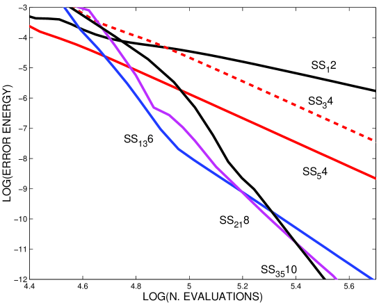
Figure 4: Average error in energy versus number of force evaluations in a double logarithmic scale for the numerical integration of the Hamiltonian system (99). It is shown performance of the most efficient non-processed symmetric-symmetric methods from Table 4.

The following numerical experiment intends to illustrate the interest of the methods designed for problems with some particular structure. For simplicity, in this numerical test we only consider fourth-order methods from different families of methods which can be used on this problem, in order to observe the benefit of tuned methods for problems with particular structures. The following methods are considered in addition to SS₃4 and SS₅4:

• S₆4: The symmetric 6-stage 4th-order method for separable problems [16] from Table 5.

• RKN₆4: The symmetric 6S_BAB 4th-order method for Nyström problems [16] from Table 6.

• NI(8,4): The 5-stage fourth-order method 5(8,4)S_BAB given in [53] from Table 8.

• RK₄4: The standard 4-stage 4th-order non-symplectic Runge-Kutta methods, used as a reference method.

Figure 5 shows in double logarithmic scale the results obtained. In the left panel we show the average error in energy versus the number of force evaluations and in the right panel we repeated the same experiment, but we measured the average error in position (computed at the same instants). For the method NI(8,4) this counting of the computational cost is not an appropriate measure. Its computational cost strongly depends on each particular problem since the evolution of $H_{0}$ has to be computed exactly (or very accurately). For simplicity, in our experiments, we have considered that one stage of NI(8,4) is twice as expensive as one evaluation of the force. We have also included as a reference the curve obtained in Fig. 4 by SS₃₅10.

Observe that in the first case the results will be largely independent of $t_{f}$ because the average error in energy does not increase secularly for symplectic integrators. For comparison, we have also included the results obtained by the standard 4-stage fourth-order Runge-Kutta method whose error in energy grows linearly and the error in positions quadratically.

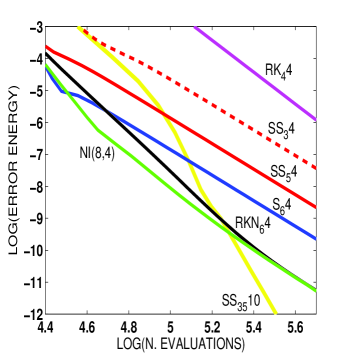
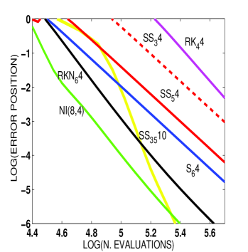
Figure 5: Average error in energy (left panel) and position (right panel) versus number of force evaluations in a double logarithmic scale for the numerical integration of the Hamiltonian system (99). The performance of different 4th-order methods from Tables 4-8 is shown. As a reference, we also shown the results obtained by the standard 4-stage fourth-order Runge-Kutta method.

Even more accurate results could be obtained as follows. As mentioned, for this particular problem, modified potentials could be used and this can be done at a very low computational cost. Then, methods from Tables 7 and 8 can be used. For instance, for the split (100) we can apply methods which incorporate modified perturbations $\exp(\varepsilon C_{h}(b,c))$ into the algorithm. Then the following map has to be evaluated:

$${\rm e}^{\varepsilon C_{h}(b,c)}p_{1} =p_{1}+h\varepsilon\left(b\frac{\displaystyle A}{\displaystyle r^{7}}-h^{2}\varepsilon c\frac{\displaystyle C}{\displaystyle(r^{7})^{2}}\right)q_{1}$$

$${\rm e}^{\varepsilon C_{h}(b,c)}p_{2} =p_{2}+h\varepsilon\left(b\frac{\displaystyle B}{\displaystyle r^{7}}-h^{2}\varepsilon c\frac{\displaystyle D}{\displaystyle(r^{7})^{2}}\right)q_{2},$$ (101)

where $A=(3/2)(\alpha(3q_{1}^{2}-2q_{2}^{2})-r^{2})$, $B=(3/2)(\alpha 5q_{1}^{2}-r^{2})$, $C=9(2r^{4}+3\alpha r^{2}(q_{2}^{2}-4q_{1}^{2})+\alpha^{2}(18q_{1}^{4}+q_{1}^{2}q_{2}^{2}-2q_{2}^{4}))$ and $D=9(2r^{4}-15\alpha r^{2}q_{1}^{2}+5\alpha^{2}q_{1}^{2}(5q_{1}^{2}+2q_{2}^{2}))$. Notice that the increment in the computational cost with respect to the evaluation of ${\rm e}^{h\varepsilon bF^{[b]}}$ (which corresponds to $c=0$) is only due to a few very simple additional operations. For this particular example, the evaluation of the modified perturbation ${\rm e}^{\varepsilon C_{h}(b,c)}$ is about a $10-20\%$ more expensive than ${\rm e}^{hbF^{[b]}}$.

As a result, more elaborated and efficient methods are obtained by considering the schemes $(n,4)$ and $(n,5)$ from Table 8 with processing (which only requires a few more code lines to program) for RKN problems and which incorporate modified potentials (see [12]).

8.2 The Schrödinger equation

As a second example we consider the one-dimensional time-dependent Schrödinger equation (26) with the Morse potential $V(x)=D\left(1-e^{-\alpha x}\right)^{2}$. We fix the parameters to the following values in atomic units (a.u.): $\mu=1745$ a.u., $D=0.2251$ a.u. and $\alpha=1.1741$ a.u., which are frequently used for modelling the HF molecule. As initial conditions we take the Gaussian wave function $\psi(x,t)=\rho\exp\big{(}-\beta(x-\bar{x})^{2}\big{)}$, with $\beta=\sqrt{k\mu}/2$, $k=2D\alpha^{2}$, $\,\bar{x}=-0.1$ and $\rho$ is a normalizing constant. Assuming that the system is defined in the interval $\,x\in[-0.8,4.32]$, we split it into $d=128$ parts of length $\Delta x=0.04$, take periodic boundary conditions and integrate along the interval $\ t\in[0,20\cdot 2\pi/w_{0}]$ with $w_{0}=\alpha\sqrt{2D/\mu}$ (see [8] for more details on the implementation of the splitting methods to this particular problem).

Figure 6 shows the error in the Euclidean norm of the vector solution at the end of the integration versus the number of FFT calls in double logarithmic scale. The integrations are done starting from a sufficiently small time step and repeating the computation by slightly increasing the time step until an overflow occurs, which we identify with the stability limit. We present the results for the following methods (in addition to the previous ones SS₁2, SS₃4 and SS₂₁8):

• RKN₁₁6: The 11-stage 6th-order method 11S_BAB-[16] from Table 6.

• GM₁₂12: The 12-stage 12th-order method from [37] tailored for linear problems with this particular structure.

• P${}_{38}2$: The 38-stage second order processed method with coefficients given in [8] tailored for linear problems with this particular structure (only the computational cost required to evaluate the kernel has been taken into consideration).

• T${}_{r}r,\ r=8,12$: $r$-stage $r$th-order Taylor methods obtained by truncating the exponential up to order $r$.

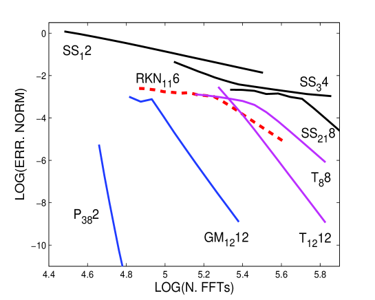
Figure 6: Error of the vector solution for the Schrödinger equation versus the number of FFT calls in a log-log scale for the symmetric-symmetric composition methods: SS_kn, for methods of order $n$ using $k$-stage compositions; RKN₁₁6 is an 11-stage 6th-order methods from [16] for Nyström problems; the 12-stage 12th-order method, GM₁₂12, from [37]; and P${}_{38}2$, a 38-stage second order processed method.

From the figure we observe that, for this numerical experiment, standard Taylor methods outperform to general symmetric-symmetric splitting methods and are also more accurate than the RKN method. This is because this problem has a very particular structure and these splitting methods are not optimized for them. However, the schemes GM₁₂12 and P${}_{38}2$ are built for linear problems with this structure and their superiority is clearly manifest. It is important to remember that Taylor methods are non-geometric integrators. The numerical experiments are carried out for a relatively short time, and the relative performances of the Taylor methods deteriorates with respect to splitting methods for longer integrations.

9 Conclusions and outlook

Splitting methods are a flexible and powerful way to solve numerically the initial value problem defined by (1) when $f$ can be decomposed into two or more parts and each of them is simpler to integrate than the original problem. This is especially true when the exact flow possesses some structural features which seems natural to reproduce at the discrete level, as happens, for instance, in Hamiltonian, Poisson, volume-preserving or time-reversible dynamical systems. They are explicit, usually simple to apply in practice and constitute an important class of geometric numerical integrators. Closely connected with splitting schemes are composition methods. In this case, the idea is to construct numerical integrators of arbitrarily high order by composing one or more basic schemes of low order with appropriately chosen coefficients. The resulting method inherits the relevant properties that the basic integrator shares with the exact solution, provided these properties are preserved by composition.

In this paper we have reviewed some of the main features of splitting and composition methods in the numerical integration of ordinary differential equations. We have presented a novel approach to get the order conditions of this class of schemes based on Lyndon words and we have seen how these order conditions particularize when coping with special classes of dynamical systems (near-integrable systems and second-order differential equations of the form $y^{\prime\prime}=g(y)$). It turns out that the number of equations to be solved increases dramatically with the order considered, as so does the complexity of the problem of finding efficient high order methods. One way to circumvent (up to a certain point) this difficulty consists in applying the processing technique, since then it is possible to design algorithms with fewer evaluations per time step. In this sense, one could say that the use of processing is perhaps the most economical path to achieve high order.

Since splitting methods are widely applied in many areas of science, it is not surprising that a great number of different schemes are available in the mathematical, physical and chemical literature. We have collected here some of the most representative integrators, classified according to the particular structure of the differential equations, the number of stages and the order of consistency, citing in each case the actual reference where the method has been first proposed.

The good qualitative behavior exhibited by splitting methods (including preservation of invariants and structures in phase space), as well as their favorable error propagation in long-time integrations can be accounted for by applying the theory of backward error analysis. Loosely speaking, the observed performance is related with the fact that the numerical solution provided by the splitting method is the exact solution of a differential equation with the same geometric properties as the original system. This interpretation constitutes in addition the basis for rigorous estimates on the numerical solution.

In contrast with standard integration methods (Runge–Kutta, multistep), whose efficiency is essentially independent of the particular differential equation considered, splitting schemes can be designed to incorporate in their formulation some of the most relevant properties of the original system. This feature has to be taken into account when comparing the efficiency of splitting methods with respect to other general purpose integrators. In this sense, Figures 4 and 5 are quite illustrative. For this particular problem, specially adapted 4th-order splitting schemes are up to 6 orders of magnitude more accurate with the same computational cost than the well known Runge–Kutta method. They even outperform other standard higher order composition integrators for a wide range of values of the step size $h$.

As an additional evidence of the extraordinary flexibility of splitting methods, we have considered the problem of designing specially tailored schemes for the numerical integration of the generalized harmonic oscillator (18). It turns out that several partial differential equations appearing in quantum mechanics, optics and electrodynamics give rise, once discretized in space, to this system with different matrices $M$ and $N$. The particular structure of this dynamical system can be exploited to build an optimized processed second order method involving a large number of stages that nevertheless is far more efficient than other integrators.

There are other issues in connection with splitting and composition methods that we have not tackled here, however, and that are also important in this context. Among them we can mention the following.

• As was remarked in the introduction, no general rule is provided here to split any given function $f$ in the differential equation (1). It turns out that, for $f$ within a certain class of ODEs, this can be done systematically, whereas for other functions one has to proceed on a case by case basis. Sometimes, several splittings are possible, and the different schemes built from them lead to the preservation of distinctive geometric properties. It makes sense, then, to classify the ODEs and their corresponding integration methods into different categories. This aspect has been analyzed in [57]. Moreover, in many physical problems there are several geometric properties that are conserved simultaneously along the evolution and it is not clear at all how to design methods preserving all of them. In that case, which one is the most relevant from a numerical point of view?

• In this paper we have only considered the initial value problem defined by eq. (1) and integration methods with constant step size $h$. Backward error analysis provides an argument why this has to be the case in geometric numerical integration: the modified equation corresponding to the numerical method depends explicitly on $h$, so that if $h$ is changed so does the modified equation and no preservation of geometric properties is guaranteed. There are problems, however, where the use of an adaptive step size is mandatory, for instance in configurations of the $N$-body problem allowing close encounters. In this case one may apply splitting methods with variable step size by using some specifically designed transformations involving the time variable, in such a way that in the new variables the resulting time step is constant (see, e.g., [3]).

• As we have shown in section 3.5, the presence of negative coefficients in splitting methods of order higher than two is unavoidable. This is not a problem when the flow of the differential equation evolves in a group (such as in the Hamiltonian case), but may be unacceptable when the ODE originates from a partial differential equation that is ill-posed for negative time progression. Several alternatives have been proposed in the literature, mainly by considering, when possible, modified potentials [4], as noted in section 4.1. One should observe, however, that the analysis done in section 3.5 does not preclude the existence of complex coefficients with positive real parts. As a matter of fact, splitting methods with complex coefficients have been developed and tested for problems in which the Hamiltonian is split into kinetic and potential energy terms [24], for the time-dependent Schrödinger equation [2], for generic parabolic equations [23] and also in the more abstract setting of evolution PDEs in analytic semigroups [42].

• An important characteristic of any numerical integration method is stability. Roughly speaking, the numerical solution provided by a stable numerical integrator does not tend to infinity when the exact solution is bounded. Although important, this feature has received considerably less attention in the specific case of splitting methods. To test the (linear) stability of the method (36), instead of the linear equation $y^{\prime}=ay$ as in the usual stability analysis for ODE integrators, one considers the harmonic oscillator $y^{\prime\prime}+\lambda^{2}y=0$, $\lambda>0$, as a model problem with a splitting of the form (11). The idea is to find the time steps for which all numerical solutions remain bounded. The integrator (36) typically will be unstable for $|h\lambda|>x_{*}$, where the parameter $x_{*}$ determines the stability threshold of the numerical scheme. In particular, for the leapfrog method one has $x_{*}=2$. Although the stability threshold imposes restrictions on the step size, in the process of building high order schemes, linear stability is not usually taken into account, ending sometimes with methods possessing such a small relative stability threshold that they are useless in practice. In this way, constructing high order splitting methods with relatively large linear stability intervals and highly accurate is of great interest. This has been achieved in reference [9] for linear systems, but remains an open problem in general.

• In section 5 we have mentioned an optimization criterion to choose the free parameters in splitting and composition methods, which consist in minimizing the Euclidean norm of the coefficients that constitute the leading error term of the method. It is clear, however, that minimizing the leading error term does not guarantee that the method thus obtained is the most efficient: it might occur that the influence of the subsequent error terms is the decisive factor in the performance of the scheme. In this sense, it would be extremely interesting to have estimates on all the error terms in the asymptotic expansion of the modified equation and get the coefficients of the method that minimize these estimates.

• The numerical analysis of second-order differential equations with oscillatory solutions has aroused much interest during the past few years. The typical test problem in this setting is the equation $q^{\prime\prime}+\Omega^{2}q=f(q)$, where $\Omega$ is a symmetric and positive definite matrix. Here the aim is to design new methods which improve in accuracy and stability the standard Störmer–Verlet integrator. We refer the reader to [41] and references therein for a comprehensive study of this problem.

• Although only ODEs have been considered here, splitting methods have been also applied with success to stochastic differential equations (SDEs). Here the aim is, as in the deterministic case, to design integration methods which automatically incorporate conservation properties the SDE possesses [61].

Acknowledgements

This work has been partially supported by Ministerio de Ciencia e Innovación (Spain) under project MTM2007-61572 (co-financed by the ERDF of the European Union). SB also aknowledges the support of the UPV through the project 20070307. We are especially grateful to Prof. Arieh Iserles for his kind invitation to write and submit this paper.

References

- [1] V. I. Arnold. Mathematical Methods of Classical Mechanics. Springer-Verlag, GTM 60, Second edition, 1989.
- [2] A.D. Bandrauk, E. Dehghanian, and H. Lu. Complex integration steps in decomposition of quantum exponential evolution operators. Chem. Phys. Lett., 419:346–350, 2006.
- [3] S. Blanes and C.J. Budd. Adaptive geometric integrators for hamiltonian problems with approximate scale invariance. SIAM J. Sci. Comput., 26:1089–1113, 2005.
- [4] S. Blanes and F. Casas. On the necessity of negative coefficients for operator splitting schemes of order higher than two. Appl. Numer. Math., 54:23–37, 2005.
- [5] S. Blanes and F. Casas. Splitting methods for non-autonomous separable dynamical systems. J. Phys. A: Math. Gen., 39:5405–5423, 2006.
- [6] S. Blanes, F. Casas, and A. Murua. On the numerical integration of ordinary differential equations by processed methods. SIAM J. Numer. Anal., 42:531–552, 2004.
- [7] S. Blanes, F. Casas, and A. Murua. Composition methods for differential equations with processing. SIAM J. Sci. Comput., 27:1817–1843, 2006.
- [8] S. Blanes, F. Casas, and A. Murua. Symplectic splitting operator methods tailored for the time-dependent Schrödinger equation. J. Chem. Phys., 124:234105, 2006.
- [9] S. Blanes, F. Casas, and A. Murua. On the linear stability of splitting methods. Found. Comp. Math., 8:357–393, 2008.
- [10] S. Blanes, F. Casas, J.A. Oteo, and J. Ros. The Magnus expansion and some of its applications. Phys. Rep., 2008. In press.
- [11] S. Blanes, F. Casas, and J. Ros. Symplectic integrators with processing: a general study. SIAM J. Sci. Comput., 21:711–727, 1999.
- [12] S. Blanes, F. Casas, and J. Ros. Processing symplectic methods for near-integrable Hamiltonian systems. Celest. Mech. and Dyn. Astro., 77:17–35, 2000.
- [13] S. Blanes, F. Casas, and J. Ros. High-order Runge–Kutta–Nyström geometric methods with processing. Appl. Numer. Math., 39:245–259, 2001.
- [14] S. Blanes, F. Casas, and J. Ros. New families of symplectic runge-kutta-nyström integration methods. In Numerical Analysis and its Applications, LNCS 1988, pages 102–109. Springer, 2001.
- [15] S. Blanes and P.C. Moan. Splitting methods for non-autonomous Hamiltonian equations. J. Comp. Phys., 170:205–230, 2001.
- [16] S. Blanes and P.C. Moan. Practical symplectic partitioned Runge–Kutta and Runge–Kutta–Nyström methods. J. Comput. Appl. Math., 142:313–330, 2002.
- [17] C.J. Budd and A. Iserles. Geometric integration: numerical solution of differential equations on manifolds. Phil. Trans. Royal Soc. A, 357:945–956, 1999.
- [18] J. Butcher. The effective order of Runge–Kutta methods. In Conference on the Numerical Solution of Differential Equations, Lecture Notes in Math. 109, pages 133–139, Berlin, 1969. Springer.
- [19] M.P. Calvo and J.M. Sanz-Serna. The development of variable-step symplectic integrators, with applications to the two-body problem. SIAM J. Sci. Comput., 14:936–952, 1993.
- [20] M.P. Calvo and J.M. Sanz-Serna. High-order symplectic Runge–Kutta–Nyström methods. SIAM J. Sci. Comput., 14:1237–1252, 1993.
- [21] J. Candy and W. Rozmus. A symplectic integration algorithm for separable Hamiltonian functions. J. Comp. Phys., 92:230–256, 1991.
- [22] F. Casas and A. Murua. An efficient algorithm for computing the Baker–Campbell–Hausdorff series and some of its applications. Technical report, Universitat Jaume I, 2008.
- [23] F. Castella, P. Chartier, S. Decombes, and G. Vilmart. Splitting methods with complex times for parabolic equations. Technical report, Université de Rennes, September 2008.
- [24] J.E. Chambers. Symplectic integrators with complex time steps. Astron. J., 126:1119–1126, 2003.
- [25] P. Chartier and A. Murua. An algebraic theory of order. Technical report, 2008. Submitted.
- [26] S.A. Chin. Symplectic integrators from composite operator factorizations. Phys. Lett. A, 226:344–348, 1997.
- [27] S.A. Chin. Structure of positive decomposition of exponential operators. Phys. Rev. E, 71:016703, 2005.
- [28] S.A. Chin and C.R. Chen. Fourth order gradient symplectic integrator methods for solving the time-dependent Schrödinger equation. J. Chem. Phys., 114:7338–7341, 2001.
- [29] L.Y. Chou and P.W. Sharp. Order 5 symplectic explicit Runge–Kutta–Nyström methods. J. Appl. Math. Decision Sci., 4:143–150, 2000.
- [30] M. Creutz and A. Gocksch. Higher-order hybrid Monte Carlo algorithms. Phys. Rev. Lett., 63:9–12, 1989.
- [31] J.M.A. Danby. Fundamentals of Celestial Mechanics. Willmann-Bell, 1988.
- [32] M.D. Feit, Jr. J.A. Fleck, and A. Steiger. Solution of the Schrödinger equation by a spectral method. J. Comp. Phys., 47:412–, 1982.
- [33] E. Forest. Sixth-order Lie group integrators. J. of Comp. Phys., 99:209–213, 1992.
- [34] E. Forest and R.D. Ruth. Fourth-order symplectic integration. Physica D, 43:105–117, 1990.
- [35] D. Goldman and T.J. Kaper. th-order operator splitting schemes and nonreversible systems. SIAM J. Numer. Anal., 33:349–367, 1996.
- [36] H. Goldstein. Classical Mechanics. Addison Wesley, Second edition, 1980.
- [37] S. Gray and D.E. Manolopoulos. Symplectic integrators tailored to the time-dependent Schrödinger equation. J. Chem. Phys., 104:7099–7112, 1996.
- [38] S. Gray and J.M. Verosky. Classical Hamiltonian structures in wave packet dynamics. J. Chem. Phys., 100:5011–5022, 1994.
- [39] J. Guckenheimer and P. Holmes, editors. Nonlinear Oscillations, Dynamical Systems, and Bifurcations of Vector Fields. Springer, 1983.
- [40] E. Hairer, Ch. Lubich, and G. Wanner. Geometric Numerical Integration. Structure-Preserving Algorithms for Ordinary Differential Equations. Springer-Verlag, 2002.
- [41] E. Hairer, Ch. Lubich, and G. Wanner. Geometric Numerical Integration. Structure-Preserving Algorithms for Ordinary Differential Equations. Springer-Verlag, Second edition, 2006.
- [42] E. Hansen and A. Ostermann. High order splitting methods for analytic semigroups exist. Technical report, Institut für Mathematik, Universität Innsbruck, 2008.
- [43] M. Hénon and C. Heiles. The applicability of the third integral of motion: some numerical experiments. Astron. J., 69:73–79, 1964.
- [44] A. Iserles, H. Z. Munthe-Kaas, S. P. Nørsett, and A. Zanna. Lie-group methods. Acta Numerica, 9:215–365, 2000.
- [45] W. Kahan and R.C. Li. Composition constants for raising the order of unconventional schemes for ordinary differential equations. Math. Comp., 66:1089–1099, 1997.
- [46] U. Kirchgraber. An ODE-solver based on the method of averaging. Numer. Math., 53:621–652, 1988.
- [47] P.-V. Koseleff. Formal Calculus for Lie Methods in Hamiltonian Mechanics. PhD thesis, Lawrence Berkeley Laboratory, 1994.
- [48] J. Laskar and P. Robutel. High order symplectic integrators for perturbed Hamiltonian systems. Celest. Mech. and Dyn. Astro., 80:39–62, 2001.
- [49] B. Leimkuhler and S. Reich. Simulating Hamiltonian Dynamics. Cambridge University Press, 2004.
- [50] X. Liu, P. Ding, J. Hong, and L. Wang. Optimization of symplectic schemes for time-dependent Schrödinger equations. Comput. Math. Appl., 50:637–, 2005.
- [51] M.A. López-Marcos, J.M. Sanz-Serna, and R.D. Skeel. Explicit symplectic integrators using Hessian-vector products. SIAM J. Sci. Comput., 18:223–238, 1997.
- [52] E. Lorenz. Deterministic nonperiodic flows. J. Atmos. Sci., 20:130–141, 1963.
- [53] R. I. McLachlan. Composition methods in the presence of small parameters. BIT, 35:258–268, 1995.
- [54] R. I. McLachlan. On the numerical integration of ordinary differential equations by symmetric composition methods. SIAM J. Numer. Anal., 16:151–168, 1995.
- [55] R. I. McLachlan. Families of high-order composition methods. Numer. Alg., 31:233–246, 2002.
- [56] R. I. McLachlan and P. Atela. The accuracy of symplectic integrators. Nonlinearity, 5:541–562, 1992.
- [57] R.I. McLachlan and R. Quispel. Splitting methods. Acta Numerica, 11:341–434, 2002.
- [58] R.I. McLachlan and R. Quispel. Geometric integrators for ODEs. J. Phys. A: Math. Gen., 39:5251–5285, 2006.
- [59] R.I. McLachlan and B. Ryland. The algebraic entropy of classical mechanics. J. Math. Phys., 44:3071–3087, 2003.
- [60] L. Meirovich. Methods of Analytical Dynamics. McGraw-Hill, 1988.
- [61] T. Misawa. A Lie algebraic approach to numerical integration of stochastic differential equations. SIAM J. Sci. Comput., 23:866–890, 2001.
- [62] A. Murua. The Hopf algebra of rooted trees, free Lie algebras, and Lie series. Found. Comp. Math., 6:387–426, 2006.
- [63] A. Murua and J. M. Sanz-Serna. Order conditions for numerical integrators obtained by composing simpler integrators. Phil. Trans. Royal Soc. A, 357:1079–1100, 1999.
- [64] D.I. Okunbor and E.J. Lu. Eight-order explicit symplectic Runge–Kutta–Nyström integrators. Technical Report CSC 94-21, Dept. of Computer Science, University of Missouri-Rolla, 1994.
- [65] D.I. Okunbor and R.D. Skeel. Canonical Runge–Kutta–Nyström methods of orders five and six. J. Comput. Appl. Math, 51:375–382, 1994.
- [66] P. J. Olver. Applications of Lie Groups to Differential Equations. GTM 107. Springer-Verlag, Second edition, 1993.
- [67] I.P. Omelyan, I.M. Mryglod, and R. Folk. On the construction of high-order force gradient algorithms for integration of motion in classical and quantum systems. Phys. Rev. E, 66:026701, 2002.
- [68] L.P. Pitaevskii and S. Stringari. Bose–Einstein Condensation. Clarendon Press, 2003.
- [69] C. Reutenauer. Free Lie algebras, volume 7 of London Math. Soc. monographs (new series). Oxford University Press, 1993.
- [70] R. Rieben, D. White, and G. Rodrigue. High-order symplectic integration methods for finite element solutions to time dependent Maxwell equations. IEEE Trans. Antennas Propagat., 52:2190–2195, 2004.
- [71] G. Rowlands. A numerical algorithm for Hamiltonian systems. J. of Comp. Phys., 97:235–239, 1991.
- [72] R. Ruth. A canonical integration technique. IEEE Trans. Nucl. Sci., 30:26–69, 1983.
- [73] J. M. Sanz-Serna and M. P. Calvo. Numerical Hamiltonian Problems. AMMC 7. Chapman & Hall, 1994.
- [74] J.M. Sanz-Serna and A. Portillo. Classical numerical integrators for wave-packet dynamics. J. Chem. Phys., 104:2349–2355, 1996.
- [75] Q. Sheng. Solving linear partial differential equations by exponential splitting. IMA J. Numer. Anal., 9:199–212, 1989.
- [76] M. Sofroniou and G. Spaletta. Derivation of symmetric composition constants for symmetric integrators. Optimization Methods Software, 20:597–613, 2005.
- [77] G. Strang. On the construction and comparison of difference schemes. SIAM J. Numer. Anal., 5:506–517, 1968.
- [78] M. Suzuki. Fractal decomposition of exponential operators with applications to many-body theories and Monte Carlo simulations. Phys. Lett. A, 146:319–323, 1990.
- [79] M. Suzuki. General theory of fractal path integrals with applications to many-body theories and statistical physics. J. Math. Phys., 32:400–407, 1991.
- [80] M. Suzuki. Hybrid exponential product formulas for unbounded operators with possible applications to Monte Carlo simulations. Phys. Lett. A, 201:425–428, 1995.
- [81] M. Suzuki and K. Umeno. Higher-order decomposition theory of exponential operators and its applications to QMC and nonlinear dynamics. In Computer Simulation Studies in Condensed-Matter Physics VI, Springer Proceedings in Physics 76, pages 74–86, Berlin, 1993. Springer.
- [82] M. Takahashi and M. Imada. Montecarlo calculation of quantum system. II. Higher order correction. J. Phys. Soc. Japan, 53:3765–3769, 1984.
- [83] Ch. Tsitouras. A tenth order symplectic Runge–Kutta–Nyström method. Celest. Mech. and Dyn. Astron., 74:223–230, 1999.
- [84] V. S. Varadarajan. Lie Groups, Lie Algebras, and Their Representations. GTM 102. Springer-Verlag, 1984.
- [85] L. Verlet. Computer “experiments” on classical fluids. I. Thermodynamical properties of Lennard–Jones molecules. Phys. Rev., 159:98–103, 1967.
- [86] J. Wisdom and M. Holman. Symplectic maps for the N-body problem. Astron. J., 102:1528–1538, 1991.
- [87] J. Wisdom, M. Holman, and J. Touma. Symplectic correctors. In Integration Algorithms and Classical Mechanics, pages 217–244, Providence, RI, 1996. American Mathematical Society.
- [88] H. Yoshida. Construction of higher order symplectic integrators. Phys. Lett. A, 150:262–268, 1990.
- [89] W. Zhu, X. Zhao, and Y. Tang. Numerical methods with high order of accuracy applied in the quantum system. J. Chem. Phys., 104:2275–, 1996.