A proximal method for composite minimization

Abstract

We consider minimization of functions that are compositions of convex or prox-regular functions (possibly extended-valued) with smooth vector functions. A wide variety of important optimization problems fall into this framework. We describe an algorithmic framework based on a subproblem constructed from a linearized approximation to the objective and a regularization term. Properties of local solutions of this subproblem underlie both a global convergence result and an identification property of the active manifold containing the solution of the original problem. Preliminary computational results on both convex and nonconvex examples are promising.

1 Introduction

We consider optimization problems of the form

$$\min_{x}\,h\big{(}c(x)\big{)},$$ (1)

where the inner function $c:\Re^{n}\to\Re^{m}$ is smooth. The outer function $h:\Re^{m}\to[-\infty,+\infty]$ may be nonsmooth, but is usually convex (even polyhedral), and sufficiently well-structured to allow us to solve, relatively easily, subproblems of the form

$$\min_{d}\,h\big{(}\Phi(d)\big{)}+\frac{\mu}{2}|d|^{2},$$ (2)

for affine maps $\Phi$ and scalars $\mu>0$ (where $|\cdot|$ denotes the Euclidean norm). We analyze a “proximal” method for the problem (1). In its simplest form, for a finite convex function $h$, the method is shown below as Algorithm 1.

Algorithm 1 ProxDescent for Finite Convex $h$

  Define constants $\tau>1$, $\sigma\in(0,1)$, and $\mu_{\mbox{\scriptsize\rm min}}>0$;

  Choose $x_{0}\in\Re^{n}$, $\mu_{0}\geq\mu_{\mbox{\scriptsize\rm min}}$;

  for $k=0,1,2,\dotsc$ do

     Set accept $\leftarrow$ false;

     while not accept do

        Find the minimizer $d$ of the function $h\big{(}c(x)+\nabla c(x)d\big{)}+{\textstyle{1\over 2}}\mu|d|^{2}$

        (terminating if $d=0$);

        if $h\big{(}c(x)\big{)}-h\big{(}c(x+d)\big{)}\geq\sigma\left[h\big{(}c(x)\big{)}-h(c(x)+\nabla c(x)d)\right]$ then

           $\mu\leftarrow\max(\mu_{\mbox{\scriptsize\rm min}},\mu/\tau)$;

           accept $\leftarrow$ true;

        else

           $\mu\leftarrow\tau\mu$;

        end if

     end while

     $x\leftarrow x+d$;

  end for

The method repeatedly solves a proximal linearized subproblem of the form

$$\min_{d}\,h_{x,\mu}(d):=h\big{(}c(x)+\nabla c(x)d\big{)}+\frac{\mu}{2}|d|^{2},$$ (3)

to find a trial step $d$, where the linear map $\nabla c(x):\Re^{n}\to\Re^{m}$ is the derivative of the map $c$ at $x$ (representable by the $m\times n$ Jacobian matrix). In the algorithmic framework that we discuss later, where the function $h$ is not restricted to being polyhedral or convex, the subproblem solution $d$ is just a first approximation to the step. If $h$ is sufficiently well-structured — an assumption we make concrete using “partial smoothness,” a generalization of the idea of an active set in nonlinear programming — we may then be able to enhance the step, possibly with the use of higher-order derivative information.

Although many important problems of the form (1) involve finite convex functions $h$, we explore extensions to broader classes of functions $h$. Specifically, we allow that

• $h$ may be extended-valued, allowing it to incorporate constraints that must be enforced;

• $h$ is “prox-regular” rather than convex.

(We note in passing that our analysis extends easily to the case where the function $c$ is defined only locally.) This broader framework requires additional technical overhead, but we point out throughout the simplifications that are available in the case of continuous convex $h$, and in particular polyhedral $h$.

1.1 Outline

In the next subsection, we discuss the building blocks from variational analysis that are used in later sections, focusing on key ideas that may be unfamiliar to many readers — “prox-regularity” and “partial smoothness” — and deferring more standard formal definitions to an Appendix. In Section 2, we describe how a wide variety of examples can be posed as composite optimization problems of the form (1). We include problems from approximation, nonlinear programming, and regularized minimization, including nonconvex examples. Given its prevalence, historical importance, and significance in building intuition and terminology, we pay particular attention to the case in which the function $h$ is finite and polyhedral. Next, in Section 3, we survey the extensive body of related work.

Section 4 contains our main theoretical tools, pertaining to the subproblem (3). We note that, since any local solution $\bar{x}$ for the problem (1) is critical (meaning that $0\in\partial(h\circ c)(\bar{x})$, where $\partial$ denotes the subdifferential), a chain rule typically implies the existence of a vector $\bar{v}$ such that

$$\bar{v}\in\partial h(\bar{c})\cap\mbox{\rm Null}(\nabla c(\bar{x})^{*}),$$ (4)

where $\bar{c}:=c(\bar{x})$ and $\mbox{}^{*}$ denotes the adjoint map. In examples, we can interpret the vector $\bar{v}$ as a Lagrange multiplier. We begin by showing that, when the current point $x$ is near the critical point $\bar{x}$, the proximal linearized subproblem (3) has a local solution $d$ of size $O(|x-\bar{x}|)$. To illuminate this idea, consider first a function $h$ that is convex, lower semicontinuous, and never $-\infty$. Assuming that the vector $c(x)+\nabla c(x)d$ lies in the domain of $h$ for some step $d\in\Re^{n}$, the subproblem (3) involves minimizing a strictly convex function with nonempty compact level sets, and thus has a unique solution $d=d(x)$. If we assume slightly more — that $c(x)+\nabla c(x)d$ lies in the relative interior of the domain of $h$ for some $d$ (as holds obviously if $h$ is continuous at $c(x)$), a standard chain rule from convex analysis implies that $d=d(x)$ is the unique solution of the following inclusion:

$$\nabla c(x)^{*}v+\mu d=0,\;\;\makebox{\rm for some $v\in\partial h\big{(}c(x)+\nabla c(x)d\big{)}$}.$$ (5)

When $h$ is prox-regular rather than convex, reasonable conditions ensure that the subproblem (3) still has a unique local solution close to zero, for $\mu$ sufficiently large, also characterized by property (5). Then, by projecting the point $x+d$ onto the inverse image under the map $c$ of the domain of the function $h$, we can obtain a step that reduces the objective.

The final part of Section 4 focuses on the common situation in which the function $h$ is partly smooth at the point $\bar{c}$ relative to a certain manifold ${\cal M}$ — a generalization of the surface defined by the active constraints in classical nonlinear programming. We give conditions guaranteeing that, when $x$ is close to $\bar{x}$, the algorithm “identifies” ${\cal M}$, in the sense that the solution $d$ of the subproblem (2) has $\Phi(d)\in{\cal M}$.

Section 5 presents the ProxDescent algorithm in full generality and proves a global convergence result. Finally, Section 6 describes some promising preliminary computational experiments, on convex and nonconvex regularized linear least-squares problems, together with a polyhedral penalty function arising from a nonlinear programming application.

1.2 Variational Analysis Tools

We begin with some important basic ideas and notation. We denote by $P_{S}(v)$ the usual Euclidean projection of a vector $v\in\Re^{m}$ onto a closed set $S\subset\Re^{m}$. The distance between $x$ and the set $S$ is

$$\mbox{\rm dist}\,(x,S)=\inf_{y\in S}|x-y|.$$

We use $B_{\epsilon}(x)$ to denote the closed Euclidean ball of radius $\epsilon$ around a point $x$.

We write $\bar{\Re}$ for the extended reals $[-\infty,+\infty]$, and consider a function $h:\Re^{m}\to\bar{\Re}$. The notion of the subdifferential of $h$ at a point $\bar{c}\in\Re^{m}$, denoted $\partial h(\bar{c})$, provides a powerful unification of the classical gradient of a smooth function and the subdifferential from convex analysis. It is a set of generalized gradient vectors, coinciding exactly with the classical convex subdifferential [39] when $h$ is lower semicontinuous and convex, and equaling $\{\nabla h(\bar{c})\}$ when $h$ is ${\cal C}^{1}$ around $\bar{c}$. For formal definitions from variational analysis, we refer the reader to standard texts such as [40] and [35]. For ease of reading, we collect such definitions (along with brief discussions) in an Appendix.

Since the notion of “prox-regularity” is crucial for our development, we quote a full definition here, from [40, Definition 13.27].

Definition 1.

A function $h:\Re^{m}\to\bar{\Re}$ is prox-regular at a point $\bar{c}\in\Re^{m}$ for a subgradient $\bar{v}\in\partial h(\bar{c})$ if $h$ is finite at $\bar{c}$, locally lower semicontinuous around $\bar{c}$, and there exists $\rho>0$ such that

$$h(c^{\prime})\geq h(c)+\langle v,c^{\prime}-c\rangle-\frac{\rho}{2}|c^{\prime}-c|^{2}$$

whenever points $c,c^{\prime}\in\Re^{m}$ are near $\bar{c}$ with the value $h(c)$ near the value $h(\bar{c})$ and for every subgradient $v\in\partial h(c)$ near $\bar{v}$. Further, $h$ is prox-regular at $\bar{c}$ if it is prox-regular at $\bar{c}$ for every $\bar{v}\in\partial h(\bar{c})$.

While this definition appears formidably technical in its generality, it holds commonly in practice. Prevalent examples include continuous functions $h$ with the property that the function $h+\kappa|\cdot|^{2}$ is convex for some constant $\kappa$. For further discussion, see the Appendix.

A weaker property than the prox-regularity of a function $h$ is “subdifferential regularity.” Formal definitions and discussion can be found in standard texts and in the Appendix. Here, we simply note that both ${\cal C}^{1}$ functions and lower semicontinuous convex functions are subdifferentially regular, as are sums of such functions.

We next turn to the idea of “partial smoothness” introduced by Lewis [30], a variational-analytic formalization of the notion of the active set in classical nonlinear programming: see also Hare and Lewis [22, Definition 2.3]. A set ${\cal M}\subset\Re^{m}$ is a manifold about a point $\bar{c}\in{\cal M}$ if it can be described locally by a collection of smooth equations with linearly independent gradients. More precisely, there exists a map $F:\Re^{m}\to\Re^{k}$ that is ${\cal C}^{2}$ around $\bar{c}$, with $\nabla F(\bar{c})$ surjective, such that points $c\in\Re^{m}$ near $\bar{c}$ lie in ${\cal M}$ if and only if $F(c)=0$. The normal space to ${\cal M}$ at $\bar{c}$, denoted $N_{{\cal M}}(\bar{c})$ is then just the range of $\nabla F(\bar{c})^{*}$.

Definition 2.

Given a manifold ${\cal M}\subset\Re^{m}$ about a point $\bar{c}$, a function $h:\Re^{m}\to\bar{\Re}$ is partly smooth at $\bar{c}$ relative to ${\cal M}$ if $h$ is subdifferentially regular at all points $c\in{\cal M}$ near $\bar{c}$, the dependence of the value $h(c)$ and the (nonempty) subdifferential $\partial h(c)$ on the point $c\in{\cal M}$ are ${\cal C}^{2}$ and continuous respectively, and furthermore the affine span of $\partial h(\bar{c})$ is a translate of the normal space $N_{{\cal M}}(\bar{c})$. We refer to ${\cal M}$ as the active manifold.

As with prox-regularity, this definition appears technical. To illustrate, consider again the example of continuous function $h$ such that $h+\kappa|\cdot|^{2}$ is convex for some $\kappa$. Since such functions are always subdifferentially regular, partial smoothness amounts to smoothness of the restriction $h|_{{\cal M}}$, continuity with respect to the point $c\in{\cal M}$ of the classical directional derivative $h^{\prime}(c;d)$ for all fixed directions $d$, and the property $h^{\prime}(\bar{c};d)\geq-h^{\prime}(\bar{c};-d)$ for all $d\in N_{{\cal M}}(\bar{c})$.

2 Examples

Our basic framework admits a wide variety of interesting problems, as we show in this section.

2.1 Approximation Problems

Example 2.1 (least squares, $\ell_{1}$, and Huber approximation).

The formulation (1) encompasses both the usual (nonlinear) least squares problem if we define $h(\cdot)=|\cdot|^{2}$, and the $\ell_{1}$ approximation problem if we define $h(\cdot)=|\cdot|_{1}$, the $\ell_{1}$ norm. Another popular robust loss function is the Huber function defined by $h(c)=\sum_{i=1}^{m}\phi(c_{i})$, where

$$\phi(c_{i})=\begin{cases}{\textstyle{1\over 2}}c_{i}^{2}&\mbox{\rm($|c_{i}|\leq T$)}\\ Tc_{i}-{\textstyle{1\over 2}}T^{2}&\mbox{\rm($|c_{i}|>T$)}.\end{cases}$$

Example 2.2 (sum of Euclidean norms).

Given a collection of smooth vector functions $g_{i}:\Re^{n}\to\Re^{m_{i}}$, for $i=1,2,\dotsc,t$, consider the problem

$$\min_{x}\,\sum_{i=1}^{t}|g_{i}(x)|.$$

We can place such problems in the form (1) by defining the smooth vector function $c:\Re^{n}\to\Re^{m_{1}}\times\Re^{m_{2}}\times\cdots\times\Re^{m_{t}}$ by $c=(g_{1},g_{2},\ldots,g_{t})$, and the nonsmooth function $h:\Re^{m_{2}}\times\cdots\times\Re^{m_{t}}\to\Re$ by

$$h(g_{1},g_{2},\ldots,g_{t})=\sum_{i=1}^{t}|g_{i}|.$$

This form is seen in facility location problems and in regularized optimization problems with group-sparse regularizers.

2.2 Nonlinear Programming Penalty Functions

Next, we consider examples motivated by penalty functions for nonlinear programming.

Example 2.3 ($\ell_{1}$ penalty function).

Consider the following nonlinear program:

$$\min\,f(x)$$ (6)

$$\mbox{\rm subject to}\;\;g_{i}(x) =0\quad(1\leq i\leq j),$$

$$g_{i}(x) \leq 0\quad(j\leq i\leq k),$$

$$x \in X,$$

where the polyhedron $X\subset\Re^{n}$ describes constraints on the variable $x$ that are easy to handle directly. The $\ell_{1}$ penalty function formulation is

$$\min_{x\in X}\,f(x)+\nu\sum_{i=1}^{j}|g_{i}(x)|+\nu\sum_{i=j+1}^{k}\max\big{(}0,g_{i}(x)\big{)},$$ (7)

where $\nu>0$ is a scalar parameter. We can express this problem in the form (1) by defining the smooth vector function

$$c(x)~{}=~{}\Big{(}f(x)\,,\,\big{(}g_{i}(x)\big{)}_{i=1}^{k}\,,\,x\Big{)}~{}\in~{}\Re\times\Re^{k}\times\Re^{n}$$

and the extended polyhedral convex function $h:\Re\times\Re^{k}\times\Re^{n}\to\bar{\Re}$ by

$$h(f,g,x)=\left\{\begin{array}[]{ll}f+\nu{\displaystyle\sum_{i=1}^{j}|g_{i}|+\nu\sum_{i=j+1}^{k}}\max(0,g_{i})&(x\in X)\\ +\infty&(x\not\in X).\end{array}\right.$$

2.3 The Finite Polyhedral Case

A generalization of the polyhedral convex function of the previous subsection is obtained by defining

$$h(c)=\max_{i\in I}\{\mbox{$\langle h_{i},c\rangle$}+\beta_{i}\},$$ (8)

where $I$ is a finite set of indices, with $h_{i}\in\Re^{m}$ and $\beta_{i}\in\Re$ for all $i\in I$. We return to this case below to illustrate much of our theory (in Sections 4.4 and 4.5, for example).

Assume that the map $c\colon\Re^{n}\to\Re^{m}$ is ${\cal C}^{1}$ around a critical point $\bar{x}\in\Re^{n}$ for the composite function $h\circ c$, and let $\bar{c}=c(\bar{x})$. Define the set of “active” indices

$$\bar{I}~{}=~{}\mbox{argmax}\big{\{}\mbox{$\langle h_{i},\bar{c}\rangle$}+\beta_{i}:i\in I\big{\}}.$$

Then, denoting convex hulls by conv, we have $\partial h(\bar{c})=\mbox{conv}\{h_{i}:i\in\bar{I}\}.$ The basic criticality condition (4) becomes existence of a vector $\lambda\in\Re^{\bar{I}}$ satisfying

$$\lambda\geq 0~{}~{}~{}\mbox{and}~{}~{}~{}\sum_{i\in\bar{I}}\lambda_{i}\left[\begin{array}[]{c}\nabla c(\bar{x})^{*}h_{i}\\ 1\end{array}\right]=\left[\begin{array}[]{c}0\\ 1\end{array}\right].$$ (9)

The subgradient $\bar{v}$ is then $\sum_{i\in\bar{I}}\lambda_{i}h_{i}$.

Compare this condition with the one obtained from the standard nonlinear programming framework, which is

$$\min_{(x,t)\in\Re^{n}\times\Re}\;t\;\;\mbox{subject to}\;\;\mbox{$\langle h_{i},c(x)\rangle$}+\beta_{i}+t\leq 0\quad(i\in I).$$ (10)

At the point $\big{(}\bar{x},-h(\bar{c})\big{)}$, the conditions (9) are just the standard first-order optimality conditions, with Lagrange multipliers $\lambda_{i}$. The fact that the vector $\bar{v}$ in the criticality condition (4) is closely identified with $\lambda$ via the relationship $\bar{v}=\sum_{i\in\bar{I}}\lambda_{i}h_{i}$ motivates our terminology “multiplier vector”.

2.4 Regularized Minimization Problems

A large family of instances of (1) arises in the area of regularized minimization, where the minimization problem has the following general form:

$$\min_{x}\,f(x)+\tau|x|_{*}$$ (11)

where $f:\Re^{n}\to\Re$ is a smooth objective, while $|x|_{*}$ is a continuous, nonnegative, usually nonsmooth function, and $\tau$ is a nonnegative regularization parameter. Such formulations arise when we seek an approximate minimizer of $f$ that is “simple” in some sense; the purpose of the second term $|x|_{*}$ is to promote this simplicity property. Larger values of $\tau$ tend to produce solutions $x$ that are simpler, but less accurate as minimizers of $f$. The problem (11) can be put into the framework (1) by defining

$$c(x)=\left[\begin{matrix}f(x)\\ x\end{matrix}\right]\in\Re^{n+1},\qquad h(f,x)=f+\tau|x|_{*}.$$ (12)

We list now some interesting cases of (11).

Example 2.4 ($\ell_{1}$-regularized minimization).

The choice $|\cdot|_{*}=|\cdot|_{1}$ in (11) tends to produce solutions $x$ that are sparse, in the sense of having relatively few nonzero components. Larger values of $\tau$ tend to produce sparser solutions. Compressed sensing is a particular area of interest, in which the objective $f$ is typically a least-squares function $f(x)=(1/2)|Ax-b|^{2}$; see [9] for a survey. Regularized least-squares problems (or equivalent constrained-optimization formulations) are also encountered in statistics; see for example the LASSO [47] and LARS [16] procedures, and basis pursuit [10].

A related application is regularized logistic regression, where again $|\cdot|_{*}=|\cdot|_{1}$, but $f$ is (the negative of) an a posteriori log likelihood function [45]. Here, the components of $x$ are weights applied to the features in a data vector. We aim to identify those features (corresponding to the nonzero locations in $x$) that are most effective in predicting a binary outcome.

Another interesting class of regularized minimization problems arises in matrix completion, where we seek an $m\times n$ matrix $X$ of smallest rank that is consistent with given knowledge of various linear combinations of the elements of $X$; see [8, 37, 7]. Much as the $\ell_{1}$ norm of a vector $x$ is used as a surrogate for cardinality of $x$ in the formulations of Example 2.4, the nuclear norm is used as a surrogate for the rank of $X$ in formulations of the matrix completion problem. The nuclear norm $|X|_{*}$ is defined as the sum of singular values of $X$, and we have the following specialization of (11):

$$\min_{X\in\Re^{m\times n}}\,{\textstyle{1\over 2}}|{\cal A}(X)-b|^{2}+\tau|X|_{*},$$ (13)

where ${\cal A}$ denotes a linear operator from $\Re^{m\times n}$ to $\Re^{p}$, and $b\in\Re^{p}$ is the observation vector. Note that the nuclear norm is a continuous and convex function of $X$.

Finally, we mention image denoising and deblurring problems, which are often posed in the form (11), where $|\cdot|_{*}$ is a total-variation regularizer [41] that induces “natural” qualities in the solution images. Specifically, the recovered images contain large areas of near-constant color or shade, separated by sharp edges.

For regularized minimization problems of the form (11), the subproblem (3) has the form

$$\min_{d}\,f(x)+\langle\nabla f(x),d\rangle+\frac{\mu}{2}|d|^{2}+\tau|x+d|_{*}.$$ (14)

An equivalent formulation can be obtained by shifting the objective and making the change of variable $z:=x+d$:

$$\min_{z}\,\frac{\mu}{2}|z-y|^{2}+\tau|z|_{*},\qquad\mbox{\rm where}\quad y=x-\frac{1}{\mu}\nabla f(x).$$ (15)

When the regularization function $|\cdot|_{*}$ is separable in the components of $x$, as when $|\cdot|_{*}=|\cdot|_{1}$ or $|\cdot|=|\cdot|_{2}^{2}$, this problem can be solved in $O(n)$ time. (This fact is key to the practical efficiency of methods based on these subproblems in compressed sensing; see [51].) For the case $|\cdot|_{*}=|\cdot|_{1}$, if we set $\alpha=\tau/\mu$, the solution of (15) is

$$z_{i}=\begin{cases}0&\mbox{\rm($|y_{i}|\leq\alpha$)}\\ y_{i}-\alpha&\mbox{\rm($y_{i}>\alpha$)}\\ y_{i}+\alpha&\mbox{\rm($y_{i}<-\alpha$)}.\end{cases}$$ (16)

This operation is known commonly as the “shrink operator.”

For matrix completion (13), the formulation (15) of the subproblem becomes

$$\min_{Z\in\Re^{m\times n}}\,\frac{\mu}{2}|Z-Y|_{F}^{2}+\tau|Z|_{*},$$ (17)

where $|\cdot|_{F}$ denotes the Frobenius norm of a matrix and

$$Y=X-\frac{1}{\mu}{\cal A}^{*}[{\cal A}(X)-b].$$ (18)

It is known (see for example [7]) that (17) can be solved by using the singular-value decomposition of $Y$. Writing $Y=U\Sigma V^{T}$, where $U$ and $V$ are orthogonal and $\Sigma=\mbox{\rm diag}(\sigma_{1},\sigma_{2},\dotsc,\sigma_{\min(m,n)})$, we have $Z=U\Sigma_{\tau/\mu}V^{T}$, where the diagonals of $\Sigma_{\tau/\mu}$ are $\max(\sigma_{i}-\tau/\mu,0)$ for $i=1,2,\dotsc,\min(m,n)$. In essence, we apply the shrink operator to the singular values of $Y$, and reconstruct $Z$ by using the orthogonal matrices $U$ and $V$ from the decomposition of $Y$.

2.5 Nonconvex Problems

Each of the examples above involves a convex outer function $h$. In principle, however, the techniques we develop here also apply to a variety of nonconvex functions. This section discusses some applications in which $h$ is nonconvex.

Example 2.5 (problems involving quadratics).

Given a general quadratic function $f:\Re^{p}\to\Re$ (possibly nonconvex) and a smooth function $c_{1}:\Re^{n}\to\Re^{p}$, consider the problem $\min_{x}\,f\big{(}c_{1}(x)\big{)}$. This problem trivially fits into the framework (1), and the function $f$, being ${\cal C}^{2}$, is everywhere prox-regular. The subproblems (2), for sufficiently large values of the parameter $\mu$, simply amount to solving a linear system.

More generally, given another general quadratic function $g:\Re^{q}\to\Re$, and another smooth function $c_{2}:\Re^{n}\to\Re^{q}$, consider the problem

$$\min_{x\in\Re^{n}}\,f\big{(}c_{1}(x)\big{)}\quad\mbox{\rm subject to}\quad g\big{(}c_{2}(x)\big{)}\leq 0.$$

We can express this problem in the form (1) by defining the smooth vector function $c=(c_{1},c_{2})$ and defining an extended-valued nonconvex function

$$h(c_{1},c_{2})=\left\{\begin{array}[]{ll}f(c_{1})&(g(c_{2})\leq 0)\\ +\infty&(g(c_{2})>0).\end{array}\right.$$

The epigraph of $h$ is

$$\big{\{}(c_{1},c_{2},t):g(c_{2})\leq 0,~{}t\geq f(c_{1})\big{\}},$$

a set defined by two smooth inequality constraints: hence $h$ is prox-regular at any point $(c_{1},c_{2})$ satisfying $g(c_{2})\leq 0$ and $\nabla g(c_{2})\neq 0$. The resulting subproblems (2) are all in the form of the standard trust-region subproblem, and hence relatively straightforward to solve quickly.

As one more example of this type, we consider the case in which the outer function $h$ is defined as the maximum of a finite collection of quadratic functions (possibly nonconvex): $h(x)=\max\{f_{i}(x):i=1,2,\dotsc,k\}$. The subproblems (2) are as follows:

$$\min\Big{\{}t:t\geq f_{i}\big{(}\Phi(d)\big{)}+\frac{\mu}{2}|d|^{2},~{}d\in\Re^{m},~{}t\in\Re,~{}i=1,2,\dotsc,k\Big{\}}.$$

where the map $\Phi$ is affine. For sufficiently large values of the parameter $\mu$, this is a quadratically-constrained convex quadratic program, which can in principle be solved efficiently by an interior point method.

To conclude, we consider three more nonconvex examples. The first, due to Mangasarian [31], is used by Jokar and Pfetsch [24] to find sparse solutions of underdetermined linear equations. The formulation of [24] can be stated in the form (11) where the regularization function $|\cdot|_{*}$ has the form

$$|x|_{*}=\sum_{i=1}^{n}(1-e^{-\alpha|x_{i}|})$$

for some parameter $\alpha>0$. It is easy to see that this function is nonconvex but prox-regular, and nonsmooth only at $x_{i}=0$.

Fan and Li [17] propose the smoothly clipped absolute deviation (SCAD) regularizer. This problem has the form (11), and behaves like the $\ell_{1}$ norm near the origin, transitioning (via a concave quadratic) to a constant for large loss values. Specifically, we have $|\cdot|_{*}=\sum_{i=1}^{n}\phi(x_{i})$, where

$$\phi(x_{i})=\begin{cases}\lambda|x_{i}|&\mbox{\rm($|x_{i}|\leq\lambda$)}\\ -(|x_{i}|^{2}-2a\lambda|x_{i}|+\lambda^{2})/\big{(}2(a-1)\big{)}&\mbox{\rm($\lambda<|x_{i}|\leq a\lambda$)}\\ (a+1)\lambda^{2}/2&\mbox{\rm($|x_{i}|>a\lambda$)}.\end{cases}$$

Here $\lambda>0$ and $a>1$ are tuning parameters. The minimum concave penalty (MCP) regularizer of Zhang [54] has a similar form, with

$$\phi(x_{i})=\begin{cases}\lambda|x_{i}|-|x_{i}|^{2}/(2a)&\mbox{\rm($|x_{i}|\leq a\lambda$)}\\ a\lambda^{2}/2&\mbox{\rm($|x_{i}|>a\lambda$)}.\end{cases}$$ (19)

SCAD and MCP have been shown to avoid the bias property associated with the $\ell_{1}$ penalty function, in which nonzero values of $x$ are skewed toward zero.

3 Related Work

We discuss here some connections of our approach with existing literature.

Convex $h$

Burke [3] uses a similar composite function to the one analyzed here, and a subproblem like (2) to calculate the search direction $d$. In contrast to our approach, the analysis in [3] is restricted to finite convex $h$, and the algorithm uses a backtracking line search to ensure descent in the composite objective at each iteration. In place of the prox term $|d|^{2}/2$ of (2), Burke uses “casting functions” that serve a similar purpose of ensuring well posedness of the subproblem. Sagastizábal [42] considers the problem (1) in which $h$ is finite, convex, and positively homogeneous. Her algorithm is based on a subproblem like (3), differing mainly in that $h$ is replaced by a lower-bounding bundle approximation. Lan [27, Section 4] discusses (1) in which $h$ and the components of $c(x)$ are all Lipschitz continuous and convex. Under certain assumptions on the smoothness of $c$, a subproblem is defined that makes use of an approximation like the $h\big{(}c(x)+\nabla c(x)d\big{)}$ of (3), but taking the maximum of such approximations over all previous iterates, not just the one from the latest iterate. Global convergence is proved [27, Proposition 1] at rates that are optimal among first-order schemes.

Polyhedral $h$

Various approaches have been proposed for the case of $h$ finite and polyhedral. One work closely related to ours is by Fletcher and Sainz de la Maza [18], who discuss an algorithm for minimization of the $\ell_{1}$ penalty function (7) for the nonlinear optimization problem (6). At each iteration, their method solves a linearized trust-region problem that can be expressed in our general notation as follows:

$$\min_{d}\,h\big{(}c(x)+\nabla c(x)d\big{)}\;\;\makebox{\rm subject to}\;\;|d|\leq\rho,$$ (20)

where $\rho$ is some trust-region radius. Note that this subproblem is closely related to our linearized subproblem (3) when the Euclidean norm is used to define the trust region. However, the $\ell_{\infty}$ norm is preferred in [18], as it allows the subproblem (20) to be expressed as a linear program. The algorithm in [18] uses the solution of (20) to estimate the active constraint manifold, then computes a step that minimizes a model of the Lagrangian function for (6) while fixing the identified constraints as equalities. An active-constraint identification result is proved ([18, Theorem 2.3]); this result is related to our Theorems 13 and 18 below.

Byrd et al. [6] describe a successive linear-quadratic programming method, based on [18], which starts with solution of the linear program (20) (with $\ell_{\infty}$ trust region) and uses it to define an approximate Cauchy point, then approximately solves an equality-constrained quadratic program (EQP) over a different trust region to enhance the step. This algorithm is implemented in the KNITRO package for nonlinear optimization as the KNITRO-ACTIVE option.

Friedlander et al. [19] solve a problem of the form (3) for the case of nonlinear programming, where $h$ is the sum of the objective function $f$ and the indicator function for the equalities and the inequalities defining the feasible region. The resulting step can be enhanced by solving an EQP.

Other related literature on composite nonsmooth optimization problems with general finite polyhedral convex functions (Section 2.3) includes the papers of Yuan [52, 53] and Wright [49]. The approaches in [53, 49] solve a linearized subproblem like (20), from which an analog of the “Cauchy point” for trust-region methods in smooth unconstrained optimization can be calculated. This calculation involves a line search along a piecewise quadratic function and is therefore more complicated than the calculation in [18], but serves a similar purpose, namely as the basis of an acceptability test for a step obtained from a higher-order model.

Regularized Form (11)

For general outer functions $h$, the theory is more complex. An early approach to regularized minimization problems of the form (11) for a lower semicontinuous convex function $|\cdot|_{*}$ is due to Fukushima and Mine [20]. They calculate a trial step at each iteration by solving the linearized problem (14).

Subproblems of the form (14) were used in compressed sensing algorithms by Wright, Nowak, and Figueiredo [51] and Hale, Yin, and Zhang [21], in conjunction with an adaptive strategy for choosing $\mu$. (Indeed, this application provided the motivation for the current study.)

Combettes and Wajs [12] study formulations similar to (11) and algorithms that use subproblems like (14). Apart from assuming convexity, their setting is more general. Convergence is proved for algorithms that use values of $\mu$ in (14) that are large enough to guarantee descent in the objective at every iteration, regardless of iterate $x$. This assumption contrasts with the adaptive approach used in [51] and in Section 5 below.

$c(x)=x$: Proximal-Point Methods

The case when the map $c$ is simply the identity has a long history. The iteration $x_{k+1}=x_{k}+d_{k}$, where $d_{k}$ minimizes the function $d\mapsto h(x_{k}+d)+\frac{\mu}{2}|d|^{2}$, is the well-known proximal point method. For lower semicontinuous convex functions $h$, convergence was proved by Martinet [32] and generalized by Rockafellar [38]. For nonconvex $h$, a good survey up to 1998 is by Kaplan and Tichatschke [25]. Pennanen [36] took an important step forward, showing in particular that if the graph of the subdifferential $\partial h$ agrees locally with the graph of the inverse of a Lipschitz function (a condition verifiable using second-order properties including prox-regularity—see Levy [29, Cor. 3.2]), then the proximal point method converges linearly if started nearby and with regularization parameter $\mu$ bounded away from zero. This result was foreshadowed in much earlier work of Spingarn [46], who gave conditions guaranteeing local linear convergence of the proximal point method for a function $h$ that is the sum of lower semicontinuous convex function and a ${\cal C}^{2}$ function, conditions which furthermore hold “generically” under perturbation by a linear function. Inexact variants of Pennanen’s approach are discussed by Iusem, Pennanen, and Svaiter [23] and Combettes and Pennanen [11]. In this current work, we make no attempt to build on this more sophisticated theory, preferring a more direct and self-contained approach.

Manifold Identification

The issue of identification of the face of a constraint set on which the solution of a constrained optimization problem lies has been the focus of numerous works. For the problem $\min_{x\in X}\,f(x)$, for a closed set $X\subset\Re^{n}$, some papers show that the projection of the point $x-(1/\mu)\nabla f(x)$ onto the feasible set $X$ (for some fixed $\mu>0$) lies on the same face as the solution $\bar{x}$, under certain nondegeneracy assumptions on the problem and geometric assumptions on $X$. Identification of so-called quasi-polyhedral faces of convex $X$ was described by Burke and Moré [5]. An extension to the nonconvex case is provided by Burke [4], who considers algorithms that work with linearizations of the constraints describing $X$. Wright [50] considers surfaces of a convex set $X$ that can be parametrized by a smooth algebraic mapping, and shows how algorithms of gradient projection type can identify such surfaces once the iterates are sufficiently close to a solution. Lewis [30] and Hare and Lewis [22] extend these identification results to the nonconvex, nonsmooth case by using concepts from nonsmooth analysis, including partly smooth functions and prox-regularity. In their setting, the concept of an identifiable face of a feasible set is extended to a certain type of manifold with respect to which the function $h$ in (1) is partly smooth (see Definition 2 above).

A rich class of convex composite functions with partly smooth structure was discussed in detail by Bonnans and Shapiro [2] and Shapiro [44]. For a detailed discussion of the relationship between that class and partial smoothness, see [1].

Alternative Subproblems

Another line of relevant work is associated with the ${\cal V}{\cal U}$ theory introduced by Lemaréchal, Oustry, and Sagastizábal [28] and subsequently elaborated by these and other authors. The focus is on minimizing convex functions $f(x)$ that, again, are partly smooth — smooth (“U-shaped”) along a certain manifold through the solution $\bar{x}$, but nonsmooth (“V-shaped”) in the transverse directions. Mifflin and Sagastizábal [43] discuss the “fast track,” which is essentially the manifold containing the solution $\bar{x}$ along which the objective is smooth. Similarly to [18], they are interested in algorithms that identify the fast track and then take a minimization step for a certain Lagrangian function along this track. It is proved in [43, Theorem 5.2] that under certain assumptions, when $x$ is near $\bar{x}$, the proximal point $x+d$ obtained by solving the problem

$$\min_{d}\,f(x+d)+\frac{\mu}{2}|d|^{2}$$ (21)

lies on the fast track. This identification result is similar to the one we prove in Section 4.5, but the calculation of $d$ is different. In our case of $f=h\circ c$, (21) becomes

$$\min_{d}\,h\big{(}c(x+d)\big{)}+\frac{\mu}{2}|d|^{2}.$$ (22)

In many applications of interest, $c$ is nonlinear, so the subproblem (22) is generally harder to solve for the step $d$ than our subproblem (3).

Mifflin and Sagastizábal [33] describe an algorithm in which an approximate solution of (21) is obtained, again for the case of a convex objective, by making use of a piecewise linear underapproximation to their objective $f$, usually constructed from a bundle of subgradients gathered at earlier iterations. Approximations to the manifold of smoothness for $f$ are constructed, and a Newton-like step for the Lagrangian is taken along this manifold. Daniilidis, Hare, and Malick [13] use the terminology “predictor-corrector” to describe algorithms of this type. Miller and Malick [34] show how algorithms of this type are related to Newton-like methods that have been proposed earlier in various contexts.

Various of the algorithms discussed above make use of curvature information for the objective on the active manifold to accelerate local convergence. The algorithmic framework that we describe in Section 5 can be modified to incorporate similar techniques, while retaining its global convergence and manifold identification properties. Algorithms with this flavor have been described in [45] for the case of $\ell_{1}$-regularized logistic regression, and [48] for $\ell_{1}$-regularized least squares.

4 Properties of the Proximal Linearized Subproblem

We show in this section that when $h$ is prox-regular at $\bar{c}$, under a mild additional assumption, the subproblem (3) has a local solution $d$ with norm $O(|x-\bar{x}|)$, when the parameter $\mu$ is sufficiently large. When $h$ is convex, this solution is the unique global solution of the subproblem. We show too that a point $x^{+}$ near $x+d$ can be found such that the objective value $h\big{(}c(x^{+})\big{)}$ is close to the prediction of the model function $h(c(x)+\nabla c(x)d)$ from (3). Further, we describe conditions under which the subproblem correctly identifies the manifold ${\cal M}$ with respect to which $h$ is partly smooth at the solution of (1).

4.1 Lipschitz Properties

We start with technical preliminaries. Allowing non-Lipschitz or extended-valued outer functions $h$ in our problem (1) is conceptually appealing, since it allows us to model constraints that must be enforced. However, this flexibility presents certain technical challenges, which we now address. We begin with a simple example, to illustrate some of the difficulties.

Example 4.1.

Define a ${\cal C}^{2}$ function $c:\Re\to\Re^{2}$ by $c(x)=(x,x^{2})$, and a lower semicontinuous convex function $h:\Re^{2}\to\bar{\Re}$ by

$$h(y,z)=\left\{\begin{array}[]{ll}y&(z\geq 2y^{2})\\ +\infty&(z<2y^{2}).\end{array}\right.$$

The composite function $h\circ c$ is simply $\delta_{\{0\}}$, the indicator function of $\{0\}$. This function has a global minimum value zero, attained uniquely by $\bar{x}=0$.

At any point $x\in\Re$, the derivative map $\nabla c(x):\Re\to\Re^{2}$ is given by $\nabla c(x)d=(d,2xd)$ for $d\in\Re$. Then, for all nonzero $x$, it is easy to check that

$$h\big{(}c(x)+\nabla c(x)d\big{)}=+\infty~{}~{}\mbox{for all}~{}d\in\Re,$$

so the corresponding proximal linearized subproblem (3) has no feasible solutions: its objective value is identically $+\infty$.

The adjoint map $\nabla c(0)^{*}:\Re^{2}\to\Re$ is given by $\nabla c(0)^{*}v=v_{1}$ for $v\in\Re^{2}$, and

$$\partial h(0,0)~{}=~{}\big{\{}v\in\Re^{2}:v_{1}=1,~{}v_{2}\leq 0\big{\}}.$$

Hence the criticality condition (4) has no solution $\bar{v}\in\Re^{2}$.

This example illustrates two fundamental difficulties. The first is theoretical: the basic criticality condition (4) may be unsolvable, essentially because the chain rule fails. The second is computational: if, implicit in the function $h$, are constraints on acceptable values for $c(x)$, then curvature in these constraints can cause infeasibility in linearizations. As we see below, resolving both difficulties requires a kind of “transversality” condition common in variational analysis.

In this section we make use of the normal cone to a set $S$ at a point $s\in S$, denoted by $N_{S}(s)$, defined in the Appendix. When $S$ is convex, it coincides exactly with the classic normal cone from convex analysis, while for smooth manifolds it coincides with the classical normal space.

The transversality condition we need involves the “horizon subdifferential” of the function $h:\Re^{m}\to\bar{\Re}$ at the point $\bar{c}\in\Re^{m}$, denoted $\partial^{\infty}h(\bar{c})$. This object, which recurs throughout our analysis, consists of a set of “horizon subgradients”, capturing information about directions in which $h$ grows faster than linearly near $\bar{c}$. (See the Appendix for a formal definition.) This idea simplifies in important special cases. If $h$ is convex, finite, and lower semicontinuous at $\bar{c}$, we have the following relationship between the subdifferential and the classical normal cone to the domain (see [40, Proposition 8.12]): $\partial^{\infty}h(\bar{c})=N_{\mbox{\scriptsize dom}\,h}(\bar{c}).$ We have further that $\partial^{\infty}h(\bar{c})=\{0\}$ if $h$ is locally Lipschitz around $\bar{c}$.

This condition holds in particular for a convex function $h$ that is continuous at $\bar{c}$.

We seek conditions guaranteeing a reasonable step in the proximal linearized subproblem (3). Our key tool is the following technical result.

Theorem 3.

Consider a lower semicontinuous function $h\colon\Re^{m}\rightarrow\bar{\Re}$, a point $\bar{z}\in\Re^{m}$ where $h(\bar{z})$ is finite, and a linear map $\bar{G}\colon\Re^{n}\rightarrow\Re^{m}$ satisfying

$$\partial^{\infty}h(\bar{z})\cap\mbox{\rm Null}(\bar{G}^{*})=\{0\}.$$

Then there exists a constant $\gamma>0$ such that, for all vectors $z\in\Re^{m}$ and linear maps $G:\Re^{n}\to\Re^{m}$ with $(z,G)$ near $(\bar{z},\bar{G})$, there exists a vector $w\in\Re^{n}$ satisfying

$$|w|\leq\gamma|z-\bar{z}|~{}~{}\mbox{and}~{}~{}h(z+Gw)\leq h(\bar{z})+\gamma|z-\bar{z}|.$$

Notice that this result is trivial if $h$ is locally Lipschitz (or in particular continuous and convex) around $\bar{z}$, since we can simply choose $w=0$. The non-Lipschitz case is harder; our proof appears below following the introduction of a variety of ideas from variational analysis whose use is confined to this subsection. We refer the reader to Rockafellar and Wets [40] or Mordukhovich [35] for further details. First, we need a “metric regularity” result, which is proved below by means of a result from Dontchev, Lewis, and Rockafellar [15]. An alternative proof, which sets the result in a broader context, appears in the Appendix.

Theorem 4 (uniform metric regularity under perturbation).

Suppose that the closed set-valued mapping $F\colon\Re^{p}\;{\lower 1.0pt\hbox{$\rightarrow$}}\kern-10.0pt\hbox{\raise 2.8pt\hbox{$\rightarrow$}}\;\Re^{q}$ is metrically regular at a point $\bar{u}\in\Re^{p}$ for a point $\bar{v}\in F(\bar{u})$: in other words, there exist positive constants $\kappa$ and $a$ such that all points $u\in B_{a}(\bar{u})$ and $v\in B_{a}(\bar{v})$ satisfy

$$\mbox{\rm dist}\,\!\big{(}u,F^{-1}(v)\big{)}\leq\kappa\,\mbox{\rm dist}\,\!\big{(}v,F(u)\big{)}.$$ (23)

Then there exist constants $\delta,\gamma>0$ such that all linear maps $H\colon\Re^{p}\rightarrow\Re^{q}$ with $\|H\|<\delta$ and all points $u\in B_{\delta}(\bar{u})$ and $v\in B_{\delta}(\bar{v})$ satisfy

$$\mbox{\rm dist}\,\!\big{(}u,(F+H)^{-1}(v)\big{)}~{}\leq~{}\gamma\,\mbox{\rm dist}\,\!\big{(}v,(F+H)(u)\big{)}.$$ (24)

Proof.

We follow the notation of the proof of [15, Theorem 3.3]. Fix any constants

$$\lambda\in(0,\kappa^{-1}),\qquad\alpha\in\left(0,\frac{a}{4}(1-\kappa\lambda)\min\{1,\kappa\}\right),\qquad\delta\in\left(0,\min\left\{\frac{\alpha}{4},\frac{\alpha}{4\kappa},\lambda\right\}\right).$$

Then the proof shows inequality (24), if we define $\gamma={\kappa}/{(1-\kappa\lambda)}$. ∎

Using this result, and given a closed set $S$ containing $0$, we identify a condition under which any vector $v$ can be projected to $S$ along the range space of a given matrix, with the difference between $v$ and its projection being bounded in terms of $|v|$. We prove this result in the Appendix.

Corollary 5.

Consider a closed set $S\subset\Re^{q}$ with $0\in S$, and a linear map $\bar{A}\colon\Re^{p}\rightarrow\Re^{q}$ satisfying

$$N_{S}(0)\cap\mbox{\rm Null}(\bar{A}^{*})=\{0\}.$$

Then there exists a constant $\gamma>0$ such that, for all vectors $v\in\Re^{q}$ and linear maps $A:\Re^{p}\to\Re^{q}$ with $(v,A)$ near $(0,\bar{A})$, the inclusion

$$v+Au\in S$$

has a solution $u\in\Re^{p}$ satisfying $|u|\leq\gamma|v|$.

We are now ready to prove the main result of this subsection.

Proof of Theorem 3. Let $S\subset\Re^{m}\times\Re$ be the epigraph of $h$, and define a map $\bar{A}\colon\Re^{n}\times\Re\rightarrow\Re^{m}\times\Re$ by $\bar{A}(z,\tau)=(\bar{G}z,\tau)$. From $\partial^{\infty}h(\bar{z})\cap\mbox{Null}(\bar{G}^{*})=\{0\}$, we have $\mbox{Null}(\bar{A}^{*})=\mbox{Null}(\bar{G}^{*})\times\{0\}$, so [40, Theorem 8.9] shows that

$$N_{S}(\bar{z},h(\bar{z}))\cap\mbox{\rm Null}(\bar{A}^{*})=\{(0,0)\}.$$

For any vector $z$ and linear map $G$ with $(z,G)$ near $(\bar{z},\bar{G})$, the vector $(z,0)\in\Re^{m}\times\Re$ is near the vector $(\bar{z},0)$ and the map $(w,\tau)\mapsto(Gw,\tau)$ is near the map $(w,\tau)\mapsto(\bar{G}w,\tau)$. The previous corollary shows the existence of a constant $\gamma>0$ such that, for all such $z$ and $G$, the inclusion

$$(z,0)+(Gw,\tau)\in S$$

has a solution satisfying $|(w,\tau)|\leq\gamma|(z-\bar{z},0)|$, and the result follows.    $\Box$

We end this subsection with another tool to be used later, whose proof (in the Appendix) is a straightforward application of standard ideas from variational analysis. Like Theorem 4, this tool concerns metric regularity, this time for a constraint system of the form $F(z)\in S$ for an unknown vector $z$, where the map $F$ is smooth, and $S$ is a closed set.

Theorem 6 (metric regularity of constraint systems).

Consider a ${\cal C}^{1}$ map $F\colon\Re^{p}\to\Re^{q}$, a point $\bar{z}\in\Re^{p}$, and a closed set $S\subset\Re^{q}$ containing the vector $F(\bar{z})$. Suppose the condition

$$N_{S}\big{(}F(\bar{z})\big{)}\cap\mbox{\rm Null}(\nabla F(\bar{z})^{*})~{}=~{}\{0\}$$

holds. Then there exists a constant $\kappa>0$ such that all points $z\in\Re^{p}$ near $\bar{z}$ satisfy the inequality

$$\mbox{\rm dist}\big{(}z,F^{-1}(S)\big{)}\leq\kappa\,\mbox{\rm dist}(F(z),S).$$

4.2 The Proximal Step

We now prove a key result. Under a standard transversality condition, and assuming the proximal parameter $\mu$ is sufficiently large (if the function $h$ is nonconvex), we show the existence of a step $d=O(|x-\bar{x}|)$ in the proximal linearized subproblem (3) with corresponding objective value close to the critical value $h(\bar{c})$.

When the outer function $h$ is locally Lipschitz (or, in particular, continuous and convex), this result and its proof simplify considerably. First, the transversality condition is automatic. Second, while the proof of the result appeals to the technical tool we developed in the previous subsection (Theorem 3), this tool is trivial in the Lipschitz case, as we noted earlier. We state the theorem in a form that encompasses both the general case and the specialization to convex $h$.

Theorem 7 (proximal step).

Consider a function $h\colon\Re^{m}\rightarrow\bar{\Re}$ and a map $c\colon\Re^{n}\rightarrow\Re^{m}$. Suppose that $c$ is ${\cal C}^{2}$ around the point $\bar{x}\in\Re^{n}$, that $h$ is prox-regular at the point $\bar{c}=c(\bar{x})$, and that the composite function $h\circ c$ is critical at $\bar{x}$. Assume the transversality condition

$$\partial^{\infty}h(\bar{c})\cap\mbox{\rm Null}(\nabla c(\bar{x})^{*})~{}=~{}\{0\}.$$ (25)

Then there exist numbers $\bar{\mu}\geq 0$, $\delta>0$, and $\bar{\rho}\geq 0$, and a mapping $d:B_{\delta}(\bar{x})\times(\bar{\mu},\infty)\to\Re^{n}$ such that the following properties hold.

• For all points $x\in B_{\delta}(\bar{x})$ and all parameter values $\mu>\bar{\mu}$, the step $d(x,\mu)$ is a local minimizer of the proximal linearized subproblem (3) with

  $$h\big{(}c(x)+\nabla c(x)d(x,\mu)\big{)}+\frac{\mu}{2}|d(x,\mu)|^{2}\leq h\big{(}c(x)\big{)},$$

  and moreover $|d(x,\mu)|\leq\bar{\rho}|x-\bar{x}|$.

• Given any sequences $x_{r}\to\bar{x}$ and $\mu_{r}>\bar{\mu}$, then if either $\mu_{r}|x_{r}-\bar{x}|^{2}\to 0$ or $h\big{(}c(x_{r})\big{)}\to h(\bar{c})$, we have

  $$h\big{(}c(x_{r})+\nabla c(x_{r})d(x_{r},\mu_{r})\big{)}\to h(\bar{c}).$$ (26)

• When $h$ is convex and lower semicontinuous, the results of parts (a) and (b) hold with $\bar{\mu}=0$.

Proof.

Without loss of generality, suppose $\bar{x}=0$ and $\bar{c}=c(0)=0$, and furthermore $h(0)=0$. By assumption, $0\in\partial(h\circ c)(0)\subset\nabla c(0)^{*}\partial h(0),$ using the chain rule [40, Thm 10.6], so there exists a vector $v\in\partial h(0)\cap\mbox{Null}(\nabla c(0)^{*}).$

We first prove part (a). By prox-regularity, there exists a constant $\rho\geq 0$ such that

$$h(z)\geq\mbox{$\langle v,z\rangle$}-\frac{\rho}{2}|z|^{2}$$ (27)

for all small vectors $z\in\Re^{m}$. Hence, there exists a constant $\delta_{1}>0$ such that $\nabla c$ is continuous on $B_{\delta_{1}}(0)$ and

$$h_{x,\mu}(d)~{}\geq~{}\mbox{$\langle v,c(x)+\nabla c(x)d\rangle$}-\frac{\rho}{2}|c(x)+\nabla c(x)d|^{2}+\frac{\mu}{2}|d|^{2}$$

for all vectors $x,d\in B_{\delta_{1}}(0)$. As a consequence, we have that

$$h_{x,\mu}(d)~{}\geq~{}\min_{|x|\leq\delta_{1},\,|d|=\delta_{1}}\,\left\{\mbox{$\langle v,c(x)+\nabla c(x)d\rangle$}-\frac{\rho}{2}|c(x)+\nabla c(x)d|^{2}\right\}+\frac{\mu}{2}|d|^{2},$$

and the term in braces is finite by continuity of $c$ and $\nabla c$ on $B_{\delta_{1}}(0)$. Hence by choosing $\bar{\mu}$ sufficiently large (certainly greater than $\rho\|\nabla c(0)\|^{2}$) we can ensure that $h_{x,\bar{\mu}}(d)\geq 1~{}~{}\mbox{whenever}~{}|x|\leq\delta_{1},~{}|d|=\delta_{1}.$ Then for $x\in B_{\delta_{1}}(0)$, $|d|=\delta_{1}$, and $\mu\geq\bar{\mu}$, we have

$$h_{x,\mu}(d)=h_{x,\bar{\mu}}(d)+\frac{1}{2}(\mu-\bar{\mu})|d|^{2}\geq 1+\frac{1}{2}(\mu-\bar{\mu})\delta_{1}^{2}.$$ (28)

Since $c$ is ${\cal C}^{2}$ at $0$, there exist constants $\beta>0$ and $\delta_{2}\in(0,\delta_{1})$ such that, for all $x\in B_{\delta_{2}}(0)$, the vector

$$z(x)=c(x)-\nabla c(x)x$$ (29)

satisfies $|z(x)|\leq\beta|x|^{2}$. Setting $G=\nabla c(x)$, $\bar{G}=\nabla c(0)$, $\bar{z}=0$, and $z=z(x)$ in Theorem 3, we obtain the following result. For some constants $\gamma>0$ and $\delta_{3}\in(0,\delta_{2})$, given any vector $x\in B_{\delta_{3}}(0)$, there exists a vector $\hat{d}(x)\in\Re^{n}$ (defined by $\hat{d}(x):=w-x$, in the notation of the theorem) satisfying

$$|x+\hat{d}(x)| \leq\gamma|z(x)|\leq\gamma\beta|x|^{2}$$

$$h\big{(}c(x)+\nabla c(x)\hat{d}(x)\big{)} \leq\gamma|z(x)|\leq\gamma\beta|x|^{2}.$$

We deduce the existence of a constant $\delta_{4}\in(0,\delta_{3})$ such that, for all $x\in B_{\delta_{4}}(0)$, the corresponding $\hat{d}(x)$ satisfies $|\hat{d}(x)|\leq|x|+\gamma\beta|x|^{2}~{}<~{}\delta_{1},$ and

$$h_{x,\mu}(\hat{d}(x)) =h(c(x)+\nabla c(x)\hat{d}(x))+\frac{\mu}{2}|\hat{d}(x)|^{2}$$

$$\leq\gamma\beta|x|^{2}+\frac{\bar{\mu}}{2}\big{(}|x|+\gamma\beta|x|^{2}\big{)}^{2}+\frac{1}{2}(\mu-\bar{\mu})\delta_{1}^{2}$$

$$<1+\frac{1}{2}(\mu-\bar{\mu})\delta_{1}^{2}.$$

The lower semicontinuous function $h_{x,\mu}$ must have a minimizer (which we denote $d(x,\mu)$) over the compact set $B_{\delta_{1}}(0)$. Since $d=0$ is feasible for $B_{\delta_{1}}(0)$, we must have $h_{x,\mu}\big{(}d(x,\mu)\big{)}\leq h_{x,\mu}(0)=h\big{(}c(x)\big{)}$. Moreover, the inequality above implies that the corresponding minimum value is majorized by $h_{x,\mu}\big{(}\hat{d}(x)\big{)}$, and thus is strictly less than $1+(1/2)(\mu-\bar{\mu})\delta_{1}^{2}$. But inequality (28) implies that this minimizer must lie in the interior of the ball $B_{\delta_{1}}(0)$; in particular, it must be an unconstrained local minimizer of $h_{x,\mu}$. By setting $\delta=\delta_{4}$, we complete the proof of the first part of (a). Notice further that for $x\in B_{\delta_{4}}(0)$, we have

$$h\big{(}c(x)+\nabla c(x)d(x,\mu)\big{)}$$ (30)

$$\qquad\qquad~{}\leq~{}h_{x,\mu}\big{(}d(x,\mu)\big{)}~{}\leq~{}h_{x,\mu}\big{(}\hat{d}(x)\big{)}~{}\leq~{}\gamma\beta|x|^{2}+\frac{\mu}{2}\big{(}|x|+\gamma\beta|x|^{2}\big{)}^{2}.$$

We now prove the remainder of part (a), that is, uniform boundedness of the ratio $|d(x,\mu)|/|x|$. Suppose there are sequences $x_{r}\in B_{\delta}(\bar{x})$ and $\mu_{r}>\bar{\mu}$ such that $|d_{r}|/|x_{r}|\to\infty$, where we use notation $d_{r}:=d(x_{r},\mu_{r})$ for brevity. Since $|d_{r}|\leq\delta_{1}$ by the arguments above, we must have $x_{r}\to 0$. By the arguments above, for all large $r$ we have the following inequalities:

$$\gamma\beta |x_{r}|^{2}+\frac{\mu_{r}}{2}\big{(}|x_{r}|+\gamma\beta|x_{r}|^{2}\big{)}^{2}$$

$$\geq h_{x_{r},\mu_{r}}(d_{r})$$

$$\geq\mbox{$\langle v,c(x_{r})+\nabla c(x_{r})d_{r}\rangle$}-\frac{\rho}{2}|c(x_{r})+\nabla c(x_{r})d_{r}|^{2}+\frac{\mu_{r}}{2}|d_{r}|^{2}.$$

Dividing each side by $(1/2)\mu_{r}|x_{r}|^{2}$ and letting $r\rightarrow\infty$, we recall the inequalities $\mu_{r}>\bar{\mu}>\rho\|\nabla c(0)\|^{2}\geq 0$ and observe that the left-hand side remains finite, while the right-hand side is eventually dominated by $(1-\rho\|\nabla c(0)\|^{2}/\mu_{r})|d_{r}|^{2}/|x_{r}|^{2}$, which approaches $\infty$, yielding a contradiction.

For part (b), suppose first that $\mu_{r}|x_{r}|^{2}\to 0$. By substituting $(x,\mu)=(x_{r},\mu_{r})$ into (30), we have that

$$\limsup\,h\big{(}c(x_{r})+\nabla c(x_{r})d_{r}\big{)}~{}\leq~{}0.$$ (31)

From part (a), we have that $|d_{r}|/|x_{r}|$ is uniformly bounded, hence $d_{r}\to 0$ and thus $c(x_{r})+\nabla c(x_{r})d_{r}\to 0$. Being prox-regular, $h$ is lower semicontinuous at $0$, so

$$\liminf\,h\big{(}c(x_{r})+\nabla c(x_{r})d_{r}\big{)}~{}\geq~{}0.$$

Combining these last two inequalities gives $h\big{(}c(x_{r})+\nabla c(x_{r})d_{r}\big{)}\to 0,$ as required.

Now suppose instead that $h\big{(}c(x_{r})\big{)}\to h(\bar{c})=0$. We have from (30) that

$$h\big{(}c(x_{r})+\nabla c(x_{r})d_{r}\big{)}\leq h_{x_{r},\mu_{r}}(d_{r})\leq h_{x_{r},\mu_{r}}(0)=h\big{(}c(x_{r})\big{)}.$$

Taking the lim sup, we again obtain (31), and the result follows as before.

For part (c), when $h$ is lower semicontinuous and convex, the argument simplifies. We set $\rho=0$ in (27) and choose the constant $\delta>0$ so the map $\nabla c$ is continuous on $B_{\delta}(0)$. For constants $\beta$ and $\gamma$ as before, Theorem 3 again guarantees the existence, for all small points $x$, of a step $\hat{d}(x)$ satisfying $h\big{(}c(x)+\nabla c(x)\hat{d}(x)\big{)}\leq\gamma\beta|x|^{2}.$ It follows that the proximal linearized objective $h_{x,\mu}$ is somewhere finite, so has compact level sets, by coercivity. Thus it has a global minimizer $d(x,\mu)$ (unique, by strict convexity), which must satisfy the inequality

$$h\big{(}c(x)+\nabla c(x)d(x,\mu)\big{)}\leq h\big{(}c(x)+\nabla c(x)\hat{d}(x)\big{)}\leq\gamma\beta|x|^{2}.$$

The remainder of the argument proceeds as before. ∎

We elaborate on Theorem 7(b) by giving a simple example of a function prox-regular at $c(\bar{x})$ such that for sequences $x_{r}\to\bar{x}$ and $\mu_{r}\to\infty$ that satisfy neither $\mu_{r}|x_{r}-\bar{x}|^{2}\to 0$ nor $h\big{(}c(x_{r})\big{)}\to h\big{(}c(\bar{x})\big{)}$, there exists a sequence of global minimizers $d_{r}:=d(x_{r},\mu_{r})$ of the subproblem (3) for which (26) is not satisfied. For a scalar $x$, take $c(x)=x$ and

$$h(c)=\begin{cases}-c&(c\leq 0)\\ 1+c&(c>0).\end{cases}$$

The unique critical point is clearly $\bar{x}=0$ with $c(\bar{x})=0$ and $h\big{(}c(\bar{x})\big{)}=0$, and this problem satisfies the assumptions of the theorem. Consider $x>0$, for which the subproblem (3) is

$$\min_{d}\,h_{x,\mu}(d)=h(x+d)+\frac{\mu}{2}d^{2}=\begin{cases}-x-d+\frac{\mu}{2}d^{2}&(x+d\leq 0)\\ 1+x+d+\frac{\mu}{2}d^{2}&(x+d>0).\end{cases}$$

When $\mu_{r}x_{r}\in(0,1]$, then $d_{r}=-x_{r}$ is the only local minimizer of $h_{x_{r},\mu_{r}}$. When $\mu_{r}x_{r}>1$, the situation is more interesting. The value $d_{r}=-\mu_{r}^{-1}$ minimizes the “positive” branch of $h_{x_{r},\mu_{r}}$, with function value $1+x_{r}-(2\mu_{r})^{-1}$, and there is a second local minimizer at $d_{r}=-x_{r}$, with function value $(\mu_{r}/2)x_{r}^{2}$. (In both cases, these minimizers satisfy the estimate $|d_{r}|=O(|x_{r}-\bar{x}|)$ proved in part (a).) Comparison of the function values show that in fact the global minimum is achieved at the former point ($d_{r}=-\mu_{r}^{-1}$) when $x_{r}>\mu_{r}^{-1}+\sqrt{2}\mu_{r}^{-1/2}$. If this step is taken, we have $x_{r}+d_{r}>0$, so the new iterate remains on the upper branch of $h$. For sequences $x_{r}=\mu_{r}^{-1}+2\mu_{r}^{-1/2}$ and $\mu_{r}\to\infty$, we thus have for the global minimizer $d_{r}=-\mu_{r}^{-1}$ of $h_{x_{r},\mu_{r}}$ that $h(c(x_{r})+\nabla c(x_{r})d_{r})>1$ for all $r$, while $h\big{(}c(\bar{x})\big{)}=0$, so that (26) does not hold. The alternative sequence of local minimizers $d_{r}=-x_{r}$ of does, however, satisfy the limit (26).

4.3 Restoring Feasibility

In the algorithmic framework to be discussed below, the basic iteration starts at a current point $x\in\Re^{n}$ such that the function $h$ is finite at the vector $c(x)$. We then solve the proximal linearized subproblem (3) to obtain the step $d=d(x,\mu)\in\Re^{n}$. Under reasonable conditions we have shown that, for $x$ near the critical point $\bar{x}$, we have $d=O(|x-\bar{x}|)$ and furthermore we know that the value of $h$ at the vector $c(x)+\nabla c(x)d$ is close to the critical value $h\big{(}c(\bar{x})\big{)}$.

The algorithmic idea is now to update the point $x$ to a new point $x+d$. When the function $h$ is Lipschitz, this update is motivated by the fact that, since the map $c$ is ${\cal C}^{2}$, we have, uniformly for $x$ near the critical point $\bar{x}$,

$$c(x+d)-(c(x)+\nabla c(x)d)~{}=~{}O(|d|^{2})$$

and hence

$$h\big{(}c(x+d)\big{)}-h\big{(}(c(x)+\nabla c(x)d)\big{)}~{}=~{}O(|d|^{2}).$$

However, if $h$ is not Lipschitz, it may not be appropriate to update $x$ to $x+d$: the value $h\big{(}c(x+d)\big{)}$ may even be infinite.

In order to take another step, we need somehow to restore the point $x+d$ to feasibility, or more generally to find a nearby point with objective value not much worse than our linearized estimate $h(c(x)+\nabla c(x)d)$. Depending on the form of the function $h$, this may or may not be easy computationally. However, as we now discuss, our fundamental transversality condition (25), guarantees that such a restoration is always possible in theory. In the next section, we refer to this restoration process as an “efficient projection.”

Theorem 8 (linear estimator improvement).

Consider a map $c\colon\Re^{n}\rightarrow\Re^{m}$ that is ${\cal C}^{2}$ around the point $\bar{x}\in\Re^{n}$, and a lower semicontinuous function $h\colon\Re^{m}\rightarrow\bar{\Re}$ that is finite at the vector $\bar{c}=c(\bar{x})$. Assume that the transversality condition (25) holds. Then there exist constants $\gamma$ and $\delta>0$ such that, for any point $x\in B_{\delta}(\bar{x})$ and any step $d\in B_{\delta}(0)\subset\Re^{n}$ for which $|h(c(x)+\nabla c(x)d)-h(\bar{c})|<\delta$, there exists a point $x^{+}\in\Re^{n}$ satisfying

$$|x^{+}-(x+d)|\leq\gamma|d|^{2}~{}~{}\mbox{and}~{}~{}h\big{(}c(x^{+})\big{)}~{}\leq~{}h(c(x)+\nabla c(x)d)+\gamma|d|^{2}.$$ (32)

Proof.

Define a ${\cal C}^{2}$ map $F\colon\Re^{n}\times\Re\to\Re^{m}\times\Re$ by $F(x,t)=(c(x),t)$. Notice that the epigraph $\mbox{epi}\,h$ is a closed set containing the vector $F\big{(}\bar{c},h(\bar{c})\big{)}$. Clearly we have

$$\mbox{Null}\Big{(}\nabla F\big{(}\bar{x},h(\bar{c})\big{)}^{*}\Big{)}~{}=~{}\mbox{Null}\big{(}\nabla c(\bar{x})^{*}\big{)}\times\{0\}.$$

Recalling the relationship (62) between $\partial^{\infty}h$ and $\mbox{epi}\,h$ at $\bar{c}$, we have

$$(y,0)\in N_{\mbox{\scriptsize epi}\,h}\big{(}\bar{c},h(\bar{c})\big{)}~{}~{}\Leftrightarrow~{}~{}y\in\partial^{\infty}h(\bar{c}).$$

Hence the transversality condition is equivalent to

$$N_{\mbox{\scriptsize epi}\,h}\big{(}\bar{c},h(\bar{c})\big{)}\cap\mbox{Null}\Big{(}\nabla F\big{(}\bar{x},h(\bar{c})\big{)}^{*}\Big{)}~{}=~{}\{0\}.$$

We next apply Theorem 6 to deduce the existence of a constant $\kappa>0$ such that, for all vectors $(u,t)$ near the vector $\big{(}\bar{c},h(\bar{c})\big{)}$ we have

$$\mbox{dist}\big{(}(u,t),F^{-1}(\mbox{epi}\,h)\big{)}~{}\leq~{}\kappa\,\mbox{dist}(F(u,t),\mbox{epi}\,h).$$

Thus there exists a constant $\delta>0$ such that, for any point $x\in B_{\delta}(\bar{x})$ and any step $d\in\Re^{n}$ satisfying $|d|\leq\delta$ and $|h(c(x)+\nabla c(x)d)-h(\bar{c})|\leq\delta$, we have

$$\mbox{dist}\Big{(}\big{(}x+d,h(c(x)+\nabla c(x)d)\big{)},F^{-1}(\mbox{epi}\,h)\Big{)}$$

$$\leq~{}\kappa\,\mbox{dist}\big{(}F\big{(}x+d,h(c(x)+\nabla c(x)d)\big{)},\mbox{epi}\,h\big{)}$$

$$=~{}\kappa\,\mbox{dist}\Big{(}\big{(}c(x+d),h(c(x)+\nabla c(x)d)\big{)},\mbox{epi}\,h\Big{)}$$

$$\leq~{}\kappa\,|c(x+d)-(c(x)+\nabla c(x)d)|,$$

since

$$\big{(}c(x)+\nabla c(x)d,h(c(x)+\nabla c(x)d)\big{)}~{}\in~{}\mbox{epi}\,h.$$

Since the map $c$ is ${\cal C}^{2}$, by reducing $\delta$ if necessary we can ensure the existence of a constant $\gamma>0$ such that the right-hand side of the above chain of inequalities is bounded above by $\gamma|d|^{2}$.

We have therefore shown the existence of a vector $(x^{+},t)\in F^{-1}(\mbox{epi}\,h)$ satisfying the inequalities $|x^{+}-(x+d)|\leq\gamma|d|^{2}$ and $|t-h(c(x)+\nabla c(x)d)|\leq\gamma|d|^{2}.$ Since $t\geq h\big{(}c(x^{+})\big{)}$, the result follows. ∎

4.4 Uniqueness of the Proximal Step and Convergence of Multipliers

Our focus in this subsection is on uniqueness of the local solution of (3) near $d=0$, uniqueness of the corresponding multiplier vector, and on showing that the solution $d(x,\mu)$ of (3) has a strictly lower subproblem objective value than $d=0$. For the uniqueness results, we strengthen the transversality condition (25) to a constraint qualification that we now introduce.

Throughout this subsection we assume that the function $h$ is prox-regular at the point $\bar{c}$. Since prox-regular functions are subdifferentially regular, the subdifferential $\partial h(\bar{c})$ is a closed and convex set in $\Re^{m}$, and its recession cone is exactly the horizon subdifferential $\partial^{\infty}h(\bar{c})$ (see [40, Corollary 8.11]). Denoting the subspace parallel to the affine span of the subdifferential by $\mbox{par}\,\partial h(\bar{c})$, we deduce that $\partial^{\infty}h(\bar{c})\subset\mbox{par}\,\partial h(\bar{c}).$ Hence the “constraint qualification” that we next consider, namely

$$\mbox{par}\,\partial h(\bar{c})\cap\mbox{\rm Null}(\nabla c(\bar{x})^{*})~{}=~{}\{0\}$$ (33)

implies the transversality condition (25).

Condition (33) is related to the linear independence constraint qualification in nonlinear programming. To illustrate, consider again the case of Section 2.3, where the function $h$ is finite and polyhedral:

$$h(c)=\max_{i\in I}\{\mbox{$\langle h_{i},c\rangle$}+\beta_{i}\}$$

for given vectors $h_{i}\in\Re^{m}$ and scalars $\beta_{i}$. Then, as we noted, $\partial h(\bar{c})=\mbox{conv}\{h_{i}:i\in\bar{I}\},$ where $\bar{I}$ is the set of active indices, so

$$\mbox{par}\,\partial h(\bar{c})~{}=~{}\Big{\{}\sum_{i\in\bar{I}}\lambda_{i}h_{i}:\sum_{i\in\bar{I}}\lambda_{i}=0\Big{\}}.$$

Thus condition (33) states

$$\sum_{i\in\bar{I}}\lambda_{i}\left[\begin{array}[]{c}\nabla c(\bar{x})^{*}h_{i}\\ 1\end{array}\right]=\left[\begin{array}[]{c}0\\ 0\end{array}\right]~{}~{}\Leftrightarrow~{}~{}\sum_{i\in\bar{I}}\lambda_{i}h_{i}=0.$$ (34)

By contrast, the linear independence constraint qualification for the corresponding nonlinear program (10) at the point $\big{(}\bar{x},-h(\bar{c})\big{)}$ is

$$\sum_{i\in\bar{I}}\lambda_{i}\left[\begin{array}[]{c}\nabla c(\bar{x})^{*}h_{i}\\ 1\end{array}\right]=\left[\begin{array}[]{c}0\\ 0\end{array}\right]~{}~{}\Leftrightarrow~{}~{}\lambda_{i}=0~{}~{}(i\in\bar{I}),$$

which is a stronger assumption than condition (34).

We now prove a straightforward technical result that addresses two issues: existence and boundedness of multipliers for the proximal subproblem (3), and the convergence of these multipliers to a unique multiplier that satisfies criticality conditions for (1), when the constraint qualification (33) is satisfied. The argument is routine but, as usual, it simplifies considerably in the case of $h$ locally Lipschitz (or in particular convex and continuous) around the point $\bar{c}$, since then the horizon subdifferential $\partial^{\infty}h$ is identically $\{0\}$ near $\bar{c}$.

Lemma 9.

Consider a function $h\colon\Re^{m}\to\bar{\Re}$ and a map $c\colon\Re^{n}\to\Re^{m}$. Suppose that $c$ is ${\cal C}^{2}$ around the point $\bar{x}\in\Re^{n}$, that $h$ is prox-regular at the point $\bar{c}=c(\bar{x})$, and that the composite function $h\circ c$ is critical at $\bar{x}$.

When the transversality condition (25) holds, then for any sequences $\mu_{r}>0$ and $x_{r}\to\bar{x}$ such that $\mu_{r}|x_{r}-\bar{x}|\to 0$, and any sequence of critical points $d_{r}\in\Re^{n}$ for the corresponding proximal linearized subproblems (3) satisfying the conditions

$$d_{r}=O(|x_{r}-\bar{x}|)~{}~{}\mbox{and}~{}~{}h\big{(}c(x_{r})+\nabla c(x_{r})d_{r}\big{)}\to h(\bar{c}),$$

there exists a bounded sequence of vectors $v_{r}\in\Re^{m}$ that satisfy

$$0 =\nabla c(x_{r})^{*}v_{r}+\mu_{r}d_{r},$$ (35a)

$$v_{r} \in\partial h\big{(}c(x_{r})+\nabla c(x_{r})d_{r}\big{)}.$$ (35b)

When the stronger constraint qualification (33) holds, in place of (25), the set of multipliers $v\in\Re^{m}$ solving the criticality condition (4), namely

$$\partial h(\bar{c})\cap\mbox{\rm Null}(\nabla c(\bar{x})^{*})$$ (36)

is in fact a singleton $\{\bar{v}\}$. Furthermore, any sequence of multipliers $\{v_{r}\}$ satisfying the conditions above converges to $\bar{v}$.

Proof.

We first assume (25), and claim that

$$\partial^{\infty}h\big{(}c(x_{r})+\nabla c(x_{r})d_{r}\big{)}\cap\mbox{\rm Null}(\nabla c(x_{r})^{*})~{}=~{}\{0\}$$ (37)

for all large $r$. Indeed, if this property should fail, then for infinitely many $r$ there would exist a unit vector $v_{r}$ lying in the intersection on the left-hand side, and any accumulation point of these unit vectors must lie in the set

$$\partial^{\infty}h(\bar{c})\cap\mbox{\rm Null}(\nabla c(\bar{x})^{*}),$$ (38)

by outer semicontinuity of the set-valued mapping $\partial^{\infty}h$ at the point $\bar{c}$ [40, Proposition 8.7], contradicting the transversality condition (25). As a consequence, we can apply the chain rule [40, Theorem 10.6] to deduce the existence of vectors $v_{r}\in\Re^{n}$ satisfying (35). This sequence must be bounded, since otherwise, after taking a subsequence, we could suppose $|v_{r}|\to\infty$ and then any accumulation point of the unit vectors $|v_{r}|^{-1}v_{r}$ would lie in the set (38), again contradicting the transversality condition. The first claim of the theorem is proved.

For the remaining claims, note first that the chain rule implies that the set (36) is nonempty. The constraint qualification (33) then implies that this set is a singleton $\{\bar{v}\}$. Using boundedness of $\{v_{r}\}$, and the fact that $\mu_{r}d_{r}\to 0$, we have by taking limits in (35) that any accumulation point of $\{v_{r}\}$ lies in (36) (by $h$-attentive outer semicontinuity of $\partial h$ at $\bar{c}$), and therefore $v_{r}\to\bar{v}$. ∎

Using Theorem 7, we show that the local minimizers of $h_{x_{r},\mu_{r}}$ satisfy the desired properties, and in addition give a strict improvement over $0$ in the subproblem (3).

Lemma 10.

Consider a function $h\colon\Re^{m}\to\bar{\Re}$ and a map $c\colon\Re^{n}\to\Re^{m}$. Suppose that $c$ is ${\cal C}^{2}$ around the point $\bar{x}\in\Re^{n}$, that $h$ is prox-regular at the point $\bar{c}=c(\bar{x})$, that the composite function $h\circ c$ is critical at $\bar{x}$, and that the transversality condition (25) holds. Then there is a constant $\bar{\mu}\geq 0$ with the following property. If $\mu_{r}>\bar{\mu}$ and $x_{r}\to\bar{x}$ are sequences such that $\mu_{r}|x_{r}-\bar{x}|\to 0$, then for all $r$ sufficiently large, we have the following.

• There is a local minimizer $d_{r}$ of $h_{x_{r},\mu_{r}}$ such that

  $$d_{r}=O(|x_{r}-\bar{x}|)\quad\mbox{\rm and}\quad h(c(x_{r})+\nabla c(x_{r})d_{r})\to h(\bar{c}).$$ (39)

• If $0\notin\partial(h\circ c)(x_{r})$ for all $r$, then $d_{r}\neq 0$ and

  $$h_{x_{r},\mu_{r}}(d_{r})<h_{x_{r},\mu_{r}}(0)$$ (40)

  for all $r$ sufficiently large.

Proof.

Part (a) follows from parts (a) and (b) of Theorem 7 when we choose $\bar{\mu}$ as in that theorem and set $d_{r}=d(x_{r},\mu_{r})$.

For part (b), we have from (39) and Lemma 9 that there exists $v_{r}$ satisfying (35). If we were to have $d_{r}=0$, these conditions would reduce to $\nabla c(x_{r})^{*}v_{r}=0$ and $v_{r}\in\partial h\big{(}c(x_{r})\big{)},$ so that $0\in\partial(h\circ c)(x_{r})$, by subdifferential regularity of $h$. Hence we must have $d_{r}\neq 0$. To prove (40), suppose for contradiction that there are sequences $\mu_{r}$, $x_{r}$ with the assumed properties such that this inequality does not hold for all $r$ sufficiently large. Without losing generality, we can assume that (40) fails to hold for every $r$. By taking limits in (35) and from boundedness of $\{v_{r}\}$, we can assume without loss of generality that $v_{r}\to\bar{v}$, for some $\bar{v}$ with $\nabla c(\bar{x})^{*}\bar{v}=0$, $\bar{v}\in\partial h(\bar{c})$, where we have used $h$-attentive outer semicontinuity of $\partial h(\cdot)$ to obtain the latter inclusion. Let $\rho$ be the constant from Definition 1 associated with $\bar{c}$ and $\bar{v}$, and choose $\bar{\mu}$ such that $\bar{\mu}>\rho\|\nabla c(\bar{x})\|^{2}$. By prox-regularity, we have

$$h\big{(}c(x_{r})\big{)} \geq h(c(x_{r})+\nabla c(x_{r})d_{r})+\mbox{$\langle v_{r},-\nabla c(x_{r})d_{r}\rangle$}-\frac{\rho}{2}|\nabla c(x_{r})d_{r}|^{2}$$

$$=h(c(x_{r})+\nabla c(x_{r})d_{r})+\mu_{r}|d_{r}|^{2}-\frac{\rho}{2}|\nabla c(x_{r})d_{r}|^{2}$$ by (35a)

$$\geq h(c(x_{r})+\nabla c(x_{r})d_{r})+\frac{\mu_{r}}{2}|d_{r}|^{2}+\frac{\mu_{r}-\rho\|\nabla c(x_{r})\|^{2}}{2}|d_{r}|^{2}$$

$$=h_{x_{r},\mu_{r}}(d_{r})+\frac{\mu_{r}-\rho\|\nabla c(x_{r})\|^{2}}{2}|d_{r}|^{2}$$ by (3)

$$>h_{x_{r},\mu_{r}}(d_{r}),$$

where the final inequality holds because of our choice of $\bar{\mu}$. Since $h_{x_{r},\mu_{r}}(0)=h\big{(}c(x_{r})\big{)}$, we have a contradiction, and the proof is complete. ∎

Returning to the assumptions of Theorem 7, but now with the constraint qualification (33) replacing the weaker transversality condition (25), we can derive local uniqueness results about critical points for the proximal linearized subproblem. When the outer function $h$ is convex, uniqueness is obvious, since then the proximal linearized objective $h_{\mu,x}$ is strictly convex for any $\mu>0$. For lower ${\cal C}^{2}$ functions, the argument is much the same: such functions have the form $g-\kappa|\cdot|^{2}$, locally, for some continuous convex function $g$, so again $h_{\mu,x}$ is locally strictly convex for large $\mu$. For general prox-regular functions, the argument requires slightly more care.

Theorem 11 (unique step).

Consider a function $h\colon\Re^{m}\rightarrow\bar{\Re}$ and a map $c\colon\Re^{n}\rightarrow\Re^{m}$. Suppose that $c$ is ${\cal C}^{2}$ around the point $\bar{x}\in\Re^{n}$, that $h$ is prox-regular at the point $\bar{c}=c(\bar{x})$, and that the composite function $h\circ c$ is critical at $\bar{x}$. Suppose further that the constraint qualification (33) holds. Then there exists $\bar{\mu}\geq 0$ such that the following properties hold. Given any sequence $\{\mu_{r}\}$ with $\mu_{r}>\bar{\mu}$ for all $r$ and any sequence $x_{r}\to\bar{x}$ such that $\mu_{r}|x_{r}-\bar{x}|\to 0$, there exists a sequence of local minimizers $d_{r}$ of $h_{x_{r},\mu_{r}}$ and a corresponding sequence of multipliers $v_{r}$ with the following properties:

$$0\in\partial h_{x_{r},\mu_{r}}(d_{r}),~{}~{}d_{r}=O(|x_{r}-\bar{x}|),~{}~{}\mbox{and}~{}~{}h\big{(}c(x_{r})+\nabla c(x_{r})d_{r}\big{)}\to h(\bar{c}),$$ (41)

as $r\to\infty$, and satisfying (35), with $v_{r}\to\bar{v}$, where $\bar{v}$ is the unique vector that solves the criticality condition (4). Moreover, $d_{r}$ is uniquely defined for all $r$ sufficiently large.

In the case of a convex, lower semicontinuous function $h:\Re^{m}\to(-\infty,+\infty]$, the result holds with $\bar{\mu}=0$.

Proof.

Existence of sequences $\{d_{r}\}$ and $\{v_{r}\}$ with the claimed properties follows from Theorem 7 and Lemma 9, where we select $\bar{\mu}$ in the same way as in Theorem 7. We need only prove the claim about uniqueness of the vectors $d_{r}$, and the final claim about the special case of $h$ convex and lower semicontinuous.

We first show the uniqueness of $d_{r}$ in the general case. Since the function $h$ is prox-regular at $c(\bar{x})$, its subdifferential $\partial h$ has a hypomonotone localization around the point $(c(\bar{x}),\bar{v})$ with constant $\rho>0$ (see the Appendix). If the uniqueness claim does not hold, we have by taking a subsequence if necessary that there is a sequence $x_{r}\to\bar{x}$ and distinct sequences of $d_{r}^{1}\neq d_{r}^{2}$ in $\Re^{n}$ satisfying the conditions

$$0\in\partial h_{x_{r},\mu_{r}}(d_{r}^{i}),~{}~{}d_{r}^{i}=O(|x_{r}-\bar{x}|)\to 0,~{}~{}\mbox{and}~{}~{}h\big{(}c(x_{r})+\nabla c(x_{r})d_{r}^{i}\big{)}\to h\big{(}c(\bar{x})\big{)},$$

as $r\to\infty$, for $i=1,2$. Lemma 9 shows the existence of sequences of vectors $v_{r}^{i}\in\Re^{n}$ satisfying

$$0 = \nabla c(x_{r})^{*}v_{r}^{i}+\mu_{r}d_{r}^{i}$$

$$v_{r}^{i} \in \partial h\big{(}c(x_{r})+\nabla c(x_{r})d_{r}^{i}\big{)},$$

for all large $r$, and furthermore $v_{r}^{i}\to\bar{v}$ for each $i=1,2$. Consequently, for all large $r$ we have

$$v_{r}^{i}\in T\big{(}c(x_{r})+\nabla c(x_{r})d_{r}^{i}\big{)}~{}~{}\mbox{for}~{}i=1,2,$$

so that

$$-\mu_{r}|d_{r}^{1}-d_{r}^{2}|^{2}~{}=~{}\mbox{$\langle v_{r}^{1}-v_{r}^{2},\nabla c(x_{r})(d_{r}^{1}-d_{r}^{2})\rangle$}~{}\geq~{}-\rho|\nabla c(x_{r})(d_{r}^{1}-d_{r}^{2})|^{2}.$$

Since $\bar{\mu}>\rho\|\nabla c(\bar{x})\|^{2}$, we have the contradiction $\rho\|\nabla c(x_{r})\|^{2}\geq\mu_{r}>\bar{\mu}>\rho\|\nabla c(\bar{x})\|^{2}$ for all large $r$.

For the special case of $h$ convex and lower semicontinuous, we have from Theorem 7(c) that unique $d_{r}$ with the properties (41) exists, for $\bar{\mu}=0$. ∎

4.5 Manifold Identification

We next work toward the identification result. Consider a sequence of points $\{x_{r}\}$ in $\Re^{n}$ converging to the critical point $\bar{x}$ of the composite function $h\circ c$, and let $\mu_{r}$ be a sequence of positive proximality parameters. Suppose now that the outer function $h$ is partly smooth at the point $\bar{c}=c(\bar{x})\in\Re^{m}$ relative to some manifold ${\cal M}\subset\Re^{m}$. Our aim is to find conditions guaranteeing that the update to the point $c(x_{r})$ predicted by minimizing the proximal linearized objective $h_{x_{r},\mu_{r}}$ lies on ${\cal M}$: in other words,

$$c(x_{r})+\nabla c(x_{r})d_{r}\in{\cal M}~{}~{}\mbox{for all large $r$,}$$

where $d_{r}$ is the unique small critical point of $h_{x_{r},\mu_{r}}$. We would furthermore like to ensure that the “efficient projection” $x^{+}$ resulting from this prediction, guaranteed by Theorem 8 (linear estimator improvement), satisfies $c(x^{+})\in{\cal M}$.

To illustrate, we return to our ongoing example from Section 2.3, the finite polyhedral function (8). If $\bar{I}$ is the active index set corresponding to the point $\bar{c}$, then it is easy to check that $h$ is partly smooth relative to the manifold

$${\cal M}~{}=~{}\big{\{}c:\mbox{$\langle h_{i},c\rangle$}+\beta_{i}=\mbox{$\langle h_{j},c\rangle$}+\beta_{j}~{}\mbox{for all}~{}i,j\in\bar{I}\big{\}}.$$

Our analysis requires one more assumption, in addition to those of Theorem 11. The basic criticality condition (4) requires the existence of a multiplier vector:

$$\partial h(\bar{c})\cap\mbox{\rm Null}(\nabla c(\bar{x})^{*})~{}\neq~{}\emptyset.$$

We now strengthen this assumption slightly, to a “strict” criticality condition:

$$\makebox{\rm ri}\big{(}\partial h(\bar{c})\big{)}\cap\mbox{\rm Null}(\nabla c(\bar{x})^{*})~{}\neq~{}\emptyset,$$ (42)

where ri denotes the relative interior of a convex set. The condition (42) is related to the strict complementarity assumption in nonlinear programming. For finite polyhedral $h$ (8), since $\partial h(\bar{c})=\mbox{conv}\{h_{i}:i\in\bar{I}\}$, we have

$$\makebox{\rm ri}\big{(}\partial h(\bar{c})\big{)}~{}=~{}\Big{\{}\sum_{i\in\bar{I}}\lambda_{i}h_{i}:\sum_{i\in\bar{I}}\lambda_{i}=1,~{}\lambda>0\Big{\}}.$$

Hence, the strict criticality condition (42) becomes the existence of a vector $\lambda\in\Re^{\bar{I}}$ satisfying

$$\lambda>0~{}~{}~{}\mbox{and}~{}~{}~{}\sum_{i\in\bar{I}}\lambda_{i}\left[\begin{array}[]{c}\nabla c(\bar{x})^{*}h_{i}\\ 1\end{array}\right]=\left[\begin{array}[]{c}0\\ 1\end{array}\right].$$ (43)

The only change from the corresponding basic criticality condition (9) is that the condition $\lambda\geq 0$ has been strengthened to $\lambda>0$, corresponding exactly to the extra requirement of strict complementarity in the nonlinear programming formulation (6).

Recall that the constraint qualification (33) implies the uniqueness of the multiplier vector $\bar{v}$, by Lemma 9. Assuming in addition the strict criticality condition (42), we then have

$$\bar{v}\in\makebox{\rm ri}\big{(}\partial h(\bar{c})\big{)}\cap\mbox{\rm Null}(\nabla c(\bar{x})^{*}).$$

We now prove a trivial modification of [22, Theorem 5.3].

Theorem 12.

Suppose the function $h\colon\Re^{m}\to\bar{\Re}$ is partly smooth at the point $\bar{c}\in\Re^{m}$ relative to the manifold ${\cal M}\subset\Re^{m}$, and is prox-regular there. Consider a subgradient $\bar{v}\in\makebox{\rm ri}\,\partial h(\bar{c})$. Suppose the sequence $\{\hat{c}_{r}\}\subset\Re^{m}$ satisfies $\hat{c}_{r}\to\bar{c}$ and $h(\hat{c}_{r})\to h(\bar{c})$. Then $\hat{c}_{r}\in{\cal M}$ for all large $r$ if and only if $\mbox{\rm dist}\big{(}\bar{v},\partial h(\hat{c}_{r})\big{)}\to 0$.

Proof.

The proof proceeds exactly as in [22, Theorem 5.3], except that instead of defining a function $g:\Re^{m}\times\Re\to\Re$ by $g(c,r)=r$, we set $g(c,r)=r-c^{T}\bar{v}$. ∎

We can now prove our main identification result.

Theorem 13.

Consider a function $h\colon\Re^{m}\rightarrow\bar{\Re}$, and a map $c\colon\Re^{n}\rightarrow\Re^{m}$ that is ${\cal C}^{2}$ around the point $\bar{x}\in\Re^{n}$. Suppose that $h$ is prox-regular at the point $\bar{c}=c(\bar{x})$, and partly smooth there relative to the manifold ${\cal M}$. Suppose further that the constraint qualification (33) and the strict criticality condition (42) both hold for the composite function $h\circ c$ at $\bar{x}$. Then there exist nonnegative constants $\hat{\mu}$ and $\gamma$ with the following property. Given any sequence $\{\mu_{r}\}$ with $\mu_{r}>\hat{\mu}$ for all $r$, and any sequence $x_{r}\to\bar{x}$ such that $\mu_{r}|x_{r}-\bar{x}|\to 0$, the local minimizer $d_{r}$ of $h_{x_{r},\mu_{r}}$ defined in Theorem 11 satisfies, for all large $r$, the condition

$$c(x_{r})+\nabla c(x_{r})d_{r}\in{\cal M},$$ (44)

and also the inequalities

$$|x^{\mbox{\scriptsize\rm new}}_{r}-(x_{r}+d_{r})|\leq\gamma|d_{r}|^{2}~{}~{}\mbox{and}~{}~{}h\big{(}c(x^{\mbox{\scriptsize\rm new}}_{r})\big{)}\leq h\big{(}c(x_{r})+\nabla c(x_{r})d_{r}\big{)}+\gamma|d_{r}|^{2},$$ (45)

hold for some point $x^{\mbox{\scriptsize\rm new}}_{r}$ with $c(x^{\mbox{\scriptsize\rm new}}_{r})\in{\cal M}$.

In the special case when $h:\Re^{m}\to(-\infty,+\infty]$ is convex and lower semicontinuous, the result holds with $\hat{\mu}=0$.

Proof.

Theorem 11 implies $d_{r}\to 0$, so $\hat{c}_{r}=c(x_{r})+\nabla c(x_{r})d_{r}\to\bar{c}.$ The theorem also shows $h(\hat{c}_{r})\to h(\bar{c})$, and that there exist multiplier vectors $v_{r}\in\partial h(\hat{c}_{r})$ satisfying $v_{r}\to\bar{v}\in\makebox{\rm ri}\,\partial h(\bar{c}).$ Since $\mbox{dist}\big{(}\bar{v},\partial h(\hat{c}_{r})\big{)}\leq|\bar{v}-v_{r}|\to 0,$ we can apply Theorem 12 to obtain property (44).

Let us now define a function $h_{{\cal M}}\colon\Re^{m}\to\bar{\Re}$, agreeing with $h$ on the manifold ${\cal M}$ and taking the value $+\infty$ elsewhere. By partial smoothness, $h_{{\cal M}}$ is the sum of a smooth function and the indicator function of ${\cal M}$, and hence $\partial^{\infty}h_{{\cal M}}(\bar{c})=N_{{\cal M}}(\bar{c})$. Partial smoothness also implies $\mbox{par}\big{(}\partial h(\bar{c})\big{)}=N_{{\cal M}}(\bar{c})$. We can therefore rewrite the constraint qualification (33) in the form $\partial^{\infty}h_{{\cal M}}(\bar{c})\cap\mbox{Null}\big{(}\nabla c(\bar{x})^{*}\big{)}=\{0\}.$ This condition allows us to apply Theorem 8 (linear estimator improvement), with the function $h_{{\cal M}}$ replacing the function $h$, to deduce the existence of the point $x^{\mbox{\scriptsize\rm new}}_{r}$, as required. ∎

5 A Proximal Descent Algorithm

We now describe Algorithm ProxDescent, a simple first-order algorithm that manipulates the proximality parameter $\mu$ in (3) to achieve a “sufficient decrease” in $h$ at each iteration. (This algorithm is shown in the figure below as Algorithm 2.) We follow our description with results concerning the global convergence behavior of this method and its ability to identify the manifold ${\cal M}$ discussed in Section 4.5.

Algorithm 2 ProxDescent

  Define constants $\tau>1$, $\sigma\in(0,1)$, and $\mu_{\mbox{\scriptsize\rm min}}>0$;

  Choose $x_{0}\in\Re^{n}$, $\mu_{0}\geq\mu_{\mbox{\scriptsize\rm min}}$;

  Set $\mu\leftarrow\mu_{0}$;

  for $k=0,1,2,\dotsc$ do

     Set accept $\leftarrow$ false;

     while not accept do

        if $d=0$ is a local minimizer of (3) then

           Terminate with $\bar{x}=x_{k}$;

        end if

        Find a local minimizer $d$ of (3) with $x=x_{k}$, that is

$$\min_{d}\,h_{x_{k},\mu}(d):=h\big{(}c(x_{k})+\nabla c(x_{k})d\big{)}+\frac{\mu}{2}|d|^{2},$$

such that $h_{x_{k},\mu}(d)<h_{x_{k},\mu}(0)$;

        if no such $d$ exists then

           $\mu\leftarrow\tau\mu$;

        else

           Derive $x^{+}$ from $x_{k}+d$ (by an efficient projection and/or other enhancements);

           if $h\big{(}c(x_{k})\big{)}-h\big{(}c(x^{+})\big{)}\geq\sigma\left[h\big{(}c(x_{k})\big{)}-h(c(x_{k})+\nabla c(x_{k})d)\right]$    and $|x^{+}-(x_{k}+d)|\leq{\textstyle{1\over 2}}|d|$ then

              $x_{k+1}\leftarrow x^{+}$;

              $d_{k}\leftarrow d$;

              $\mu_{k}\leftarrow\mu$;

              $\mu\leftarrow\max(\mu_{\mbox{\scriptsize\rm min}},\mu/\tau)$;

              accept $\leftarrow$ true;

           else

              $\mu\leftarrow\tau\mu$;

           end if

        end if

     end while

  end for

A few remarks about Algorithm ProxDescent are in order. First, we are not specific about the derivation of $x^{+}$ from $x_{k}+d$, but we assume that the “efficient projection” technique that is the basis of Theorem 8 is used when possible. Lemma 10 indicates that for $\mu$ sufficiently large and $x$ near a critical point $\bar{x}$ of $h\circ c$, it is indeed possible to find a local solution $d$ of (3) which satisfies $h_{x,\mu}(d)<h_{x,\mu}(0)$ as required by the algorithm, and which also satisfies the conditions of Theorem 8. Lemma 15 below shows further that the new point $x^{+}$ satisfies the acceptance tests in the algorithm. However, Lemma 15 is more general in that it also gives conditions for acceptance of the step when $x_{k}$ is not in a neighborhood of a critical point of $h\circ c$.

Second, we note that the framework allows $x^{+}$ to be improved further. For example, we could use higher-order derivatives of $c$ to take a further step along the manifold of $h$ identified by the subproblem (3) (analogous to an “EQP step” in nonlinear programming) and reset $x^{+}$ accordingly if this step produces a reduction in $h\circ c$. We discuss this point further at the end of the section.

We start our convergence analysis with a technical result showing that in the neighborhood of a non-critical point $\bar{x}$, and for bounded $\mu$, the steps $d$ do not become too short.

Lemma 14.

Consider a function $h\colon\Re^{m}\rightarrow\bar{\Re}$ and a map $c\colon\Re^{n}\rightarrow\Re^{m}$. Let $\bar{x}$ be such that: $c$ is ${\cal C}^{1}$ near $\bar{x}$; $h$ is finite at the point $\bar{c}=c(\bar{x})$ and subdifferentially regular there; the transversality condition (25) holds; but the criticality condition (4) is not satisfied. Then there exists a quantity $\epsilon>0$ such that for any sequence $x_{r}\to\bar{x}$ with $h\big{(}c(x_{r})\big{)}\to h(\bar{c})$, and any sequence $\{\mu_{r}\}$ with $\mu_{r}\geq\mu_{\mbox{\scriptsize\rm min}}$, any sequence of critical points $d_{r}$ of $h_{x_{r},\mu_{r}}$ satisfying $h_{x_{r},\mu_{r}}(d_{r})\leq h_{x_{r},\mu_{r}}(0)$ must also satisfy $\liminf_{r}\mu_{r}|d_{r}|\geq\epsilon$.

Proof.

If the result were not true, there would exist sequences $x_{r}$, $\mu_{r}$, and $d_{r}$ as above except that $\mu_{r}d_{r}\to 0$. We would then have $0\leq|d_{r}|\leq\mu_{r}|d_{r}|/\mu_{\mbox{\scriptsize\rm min}}\to 0$. Noting that $h(c(x_{r})+\nabla c(x_{r})d_{r})\to h(\bar{c})$ (using lower semicontinuity and the fact that the left-hand side is dominated by $h\big{(}c(x_{r})\big{)}$, which converges to $h(\bar{c})$), we have that

$$\partial^{\infty}h\big{(}c(x_{r})+\nabla c(x_{r})d_{r}\big{)}\cap\mbox{\rm Null}(\nabla c(x_{r})^{*})~{}=~{}\{0\},$$

for all $r$ sufficiently large. (If this were not true, we could use an $h$-attentive outer semicontinuity argument based on [40, Proposition 8.7] to deduce that $\partial^{\infty}h(\bar{c})\cap\mbox{\rm Null}(\nabla c(\bar{x})^{*})$ contains a nonzero vector, thus violating the transversality condition (25).) Hence, we can apply the chain rule and deduce that there are multiplier vectors $v_{r}$ such that (35) is satisfied, that is,

$$0 =\nabla c(x_{r})^{*}v_{r}+\mu_{r}d_{r},$$

$$v_{r} \in\partial h\big{(}c(x_{r})+\nabla c(x_{r})d_{r}\big{)},$$

for all sufficiently large $r$. If the sequence $\{v_{r}\}$ is unbounded, we can assume without loss of generality that $|v_{r}|\to\infty$. Any accumulation point of the sequence $v_{r}/|v_{r}|$ would be a unit vector in the set $\partial^{\infty}h(\bar{c})\cap\mbox{\rm Null}(\nabla c(\bar{x})^{*})$, contradicting (25). Hence, the sequence $\{v_{r}\}$ is bounded, so by taking limits in the conditions above and using $\mu_{r}d_{r}\to 0$ and outer semicontinuity of $\partial h(c)$ at $\bar{c}$, we can identify a vector $\bar{v}$ such that $\bar{v}\in\partial h(\bar{c})\cap\mbox{\rm Null}(\nabla c(\bar{x})^{*})$. Using the chain rule and subdifferential regularity, this contradicts non-criticality of $\bar{x}$. ∎

The next result makes use of the efficient projection mechanism of Theorem 8. When the conditions of this theorem are satisfied, we show that Algorithm ProxDescent can perform the projection to obtain the point $x_{k}^{+}$ in such a way that (32) is satisfied.

Lemma 15.

Consider a function $h\colon\Re^{m}\rightarrow\bar{\Re}$ and a map $c\colon\Re^{n}\rightarrow\Re^{m}$ that is ${\cal C}^{2}$ around a point $\bar{x}\in\Re^{n}$. Assume that $h$ lower semicontinuous and finite at $\bar{c}=c(\bar{x})$ and that transversality condition (25) holds at $\bar{x}$ and $\bar{c}$. Then there exist constants $\tilde{\mu}>0$ and $\tilde{\delta}>0$ with the following property: For any $x\in B_{\tilde{\delta}}(\bar{x})$, $d\in B_{\tilde{\delta}}(0)$, and $\mu\geq\tilde{\mu}$ such that

$$h_{x,\mu}(d)\leq h_{x,\mu}(0),\qquad|h(c(x)+\nabla c(x)d)-h\big{(}c(\bar{x})\big{)}|<\tilde{\delta},$$ (46)

there is a point $x^{+}\in\Re^{n}$ such that

$$h\big{(}c(x)\big{)}-h\big{(}c(x^{+})\big{)} \geq\sigma\big{[}h\big{(}c(x)\big{)}-h\big{(}c(x)+\nabla c(x)d\big{)}\big{]},$$ (47a)

$$|x^{+}-(x+d)| \leq{\textstyle{1\over 2}}|d|.$$ (47b)

Proof.

Define $\delta$ and $\gamma$ as in Theorem 8 and set $\tilde{\delta}=\min\big{(}\delta,1/(2\gamma)\big{)}$. By applying Theorem 8, we obtain a point $x^{+}$ for which $|x^{+}-(x+d)|\leq\gamma|d|^{2}\leq{\textstyle{1\over 2}}|d|$ (thus satisfying (47b)) and $h\big{(}c(x^{+})\big{)}\leq h(c(x)+\nabla c(x)d)+\gamma|d|^{2}$. Also note that because of $h_{x,\mu}(d)\leq h_{x,\mu}(0)$, we have

$$h(c(x)+\nabla c(x)d)+\frac{\mu}{2}|d|^{2}\leq h\big{(}c(x)\big{)}$$

and hence

$$|d|^{2}\leq\frac{2}{\mu}\left[h\big{(}c(x)\big{)}-h(c(x)+\nabla c(x)d)\right].$$

We therefore have

$$h\big{(}c(x)\big{)}-h\big{(}c(x^{+})\big{)} \geq h\big{(}c(x)\big{)}-h(c(x)+\nabla c(x)d)-\gamma|d|^{2}$$

$$\geq\left[h\big{(}c(x)\big{)}-h(c(x)+\nabla c(x)d)\right]\left(1-\frac{2\gamma}{\mu}\right).$$

By choosing $\tilde{\mu}$ large enough that $1-2\gamma/\tilde{\mu}>\sigma$, we obtain (47a). ∎

We also need the following elementary lemma.

Lemma 16.

For any constants $\tau>1$ and $\rho>0$ and any positive integer $t$, we have

$$\min\Big{\{}\sum_{i=1}^{t}\alpha_{i}^{2}\tau^{i}:\sum_{i=1}^{t}\alpha_{i}\geq\rho,~{}\alpha\in\Re^{t}_{+}\Big{\}}~{}~{}>~{}~{}\rho^{2}(\tau-1).$$

Proof.

By scaling, we can suppose $\rho=1$. Clearly the optimal solution of this problem must lie on the hyperplane $H=\{\alpha:\sum_{i}\alpha_{i}=1\}$. The objective function is convex, and its gradient at the point $\bar{\alpha}\in H$ defined by

$$\bar{\alpha}_{i}=\frac{\tau^{1-i}-\tau^{-i}}{1-\tau^{-t}}>0$$

is easily checked to be orthogonal to $H$. Hence $\bar{\alpha}$ is optimal, and the corresponding optimal value is easily checked to be strictly larger than $\tau-1$. ∎

For the main convergence result, we make the additional assumption that $h$ can be bounded below, globally, by a (concave) quadratic function, that is,

$$h(c)\geq h_{0}-q_{0}|c|^{2}\quad\mbox{for all $c\in\Re^{m}$},$$ (48)

for some scalars $h_{0}$ and $q_{0}\geq 0$. Such functions are called prox-bounded [40]. This assumption holds for all $h$ considered in the examples of Section 2. The other assumptions made on $h$, $c$, and $\bar{x}$ in the theorem below allow us to apply both Lemmas 14 and 15.

Theorem 17 (global convergence).

Consider a function $h\colon\Re^{m}\rightarrow\bar{\Re}$ and a map $c\colon\Re^{n}\rightarrow\Re^{m}$. Suppose that the sequence $\big{(}x_{k},h\big{(}c(x_{k})\big{)}\big{)}$ generated by Algorithm ProxDescent has an accumulation point at $\big{(}\bar{x},h(\bar{c})\big{)}$, where $\bar{c}:=c(\bar{x})$. Suppose that $c$ is ${\cal C}^{2}$ near $\bar{x}$, that $h$ is subdifferentially regular (thus lower semicontinuous) at $\bar{c}$ and is prox-bounded, and that the transversality condition (25) holds at $\bar{x}$. Then the criticality condition (4) is satisfied at $\bar{x}$.

Proof.

Suppose for contradiction that $\big{(}\bar{x},h(\bar{c})\big{)}$ is an accumulation point but is not critical. Since the sequence $\{h\big{(}c(x_{r})\big{)}\}$ generated by the algorithm is monotonically decreasing, we have $h\big{(}c(x_{r})\big{)}\downarrow h(\bar{c})$. By the acceptance test in the algorithm and the definition of $h_{x,\mu}$ in (3), we have that

$$h\big{(}c(x_{r+1})\big{)} \leq h\big{(}c(x_{r})\big{)}-\sigma\big{[}h\big{(}c(x_{r})\big{)}-h\big{(}c(x_{r})+\nabla c(x_{r})d_{r}\big{)}\big{]}$$

$$\leq h\big{(}c(x_{r})\big{)}-\sigma\frac{\mu_{r}}{2}|d_{r}|^{2}.$$ (49)

We thus have

$$h\big{(}c(x_{0})\big{)}-h\big{(}c(\bar{x})\big{)} \geq\sum_{r=0}^{\infty}h\big{(}c(x_{r})\big{)}-h\big{(}c(x_{r+1})\big{)}$$

$$\geq\frac{\sigma}{2}\sum_{r=1}^{\infty}\mu_{r}|d_{r}|^{2}~{}\geq~{}\frac{\sigma}{2}\mu_{\mbox{\scriptsize\rm min}}\sum_{r=1}^{\infty}|d_{r}|^{2},$$

which implies that $d_{r}\to 0$. Further, we have that

$$|h(c(x_{r})+ \nabla c(x_{r})d_{r})-h(\bar{c})|$$

$$\leq\left[h\big{(}c(x_{r})\big{)}-h(c(x_{r})+\nabla c(x_{r})d_{r})\right]+\left[h\big{(}c(x_{r})\big{)}-h(\bar{c})\right]$$

$$\leq\sigma^{-1}\left[h\big{(}c(x_{r})\big{)}-h\big{(}c(x_{r+1})\big{)}\right]+\left[h\big{(}c(x_{r})\big{)}-h(\bar{c})\right]\to 0.$$ (50)

Because $\bar{x}$ is an accumulation point, we can define a subsequence of indices $r_{j}$, $j=0,1,2,\dotsc$ such that $\lim_{j\to\infty}x_{r_{j}}=\bar{x}$. The corresponding sequence of regularization parameters $\mu_{r_{j}}$ must be unbounded, since Lemma 14 indicates that $\liminf_{j}\mu_{r_{j}}|d_{r_{j}}|\geq\epsilon>0$. Defining $\tilde{\mu}$ and $\tilde{\delta}$ as in Lemma 15, we can assume without loss of generality that $\mu_{r_{j}}>\tau\tilde{\mu}$ and $\mu_{r_{j+1}}>\mu_{r_{j}}$ for all $j$. Moreover, since $x_{r_{j}}\to\bar{x}$ and $d_{r}\to 0$, and using (50), we can assume that

$$x_{r_{j}} \in B_{\tilde{\delta}/2}(\bar{x}), j=0,1,2,\dotsc$$ for , (51a)

$$d_{r} \in B_{\tilde{\delta}}(0), r>r_{0}$$ for all , (51b)

$$\big{|}h(c(x_{r})+\nabla c(x_{r})d_{r} )-h(\bar{c})\big{|}\leq\tilde{\delta}, r>r_{0}$$ for all . (51c)

Suppose first that there are infinitely many $r_{j}$, $j=0,1,2,\dotsc$, such that $\mu$ is increased in an inner iteration of iteration $r_{j}$. Without loss of generality, we can assume that this behavior happens for all $r_{j}$, $j=0,1,2,\dotsc$. We consider reasons why the previously tried value $\mu_{r_{j}}/\tau$ would have been rejected. The first possible reason for rejection is that (3) does not have a local minimizer for $x=x_{r_{j}}$ and $\mu=\mu_{r_{j}}/\tau$. Because of (48), we have

$$h\big{(}c(x_{r_{j}})+ \nabla c(x_{r_{j}})d\big{)}+\frac{\mu_{r_{j}}}{2\tau}|d|^{2}$$

$$\geq h_{0}-q_{0}\big{|}c(x_{r_{j}})+\nabla c(x_{r_{j}})d\big{|}^{2}+\frac{\mu_{r_{j}}}{2\tau}|d|^{2}$$

$$\geq\left[h_{0}-2q_{0}|c(x_{r_{j}})|^{2}\right]+\left[\frac{\mu_{r_{j}}}{2\tau}-2q_{0}|\nabla c(x_{r_{j}})|^{2}\right]|d|^{2}$$

$$\geq\bar{h}_{0}+\left(\frac{\mu_{r_{j}}}{2\tau}-\bar{q}_{0}\right)|d|^{2},$$

where the last inequality follows from (51a) and smoothness of $c$. We conclude that $h_{x_{r_{j}},\mu_{r_{j}}/\tau}$ has bounded level sets for all $\mu_{r_{j}}$ sufficiently large, thus by lower semicontinuity of $h$, it attains a minimizer [40, Theorem 1.9]. Note that $d=0$ is not the minimizer (otherwise, ProxDescent would have terminated), so at least one of the local minimizers that exists has $h_{x_{r_{j}},\mu_{r_{j}}/\tau}(d)<h_{x_{r_{j}},\mu_{r_{j}}/\tau}(0)$,

We can thus assume that a local minimizer $\hat{d}_{r_{j}}$ is found at $x=x_{r_{j}}$ and $\mu=\mu_{r_{j}}/\tau$. If $\lim_{j}\hat{d}_{r_{j}}=0$, we have from $h(c(x_{r_{j}})+\nabla c(x_{r_{j}})\hat{d}_{r_{j}})\leq h(c(x_{r_{j}}))\downarrow h(c(\bar{x}))$, the fact that $x_{r_{j}}\to\bar{x}$, and lower semicontinuity of $h$ that $h(c(x_{r_{j}})+\nabla c(x_{r_{j}})\hat{d}_{r_{j}})\to h(c(\bar{x}))$. Thus, all conditions of Lemma 15 are satisfied, by $x=x_{r_{j}}$, $d=\hat{d}_{r_{j}}$, $\mu=\mu_{r_{j}}/\tau$, so it follows from this lemma that a step would have been taken and $\mu$ would not have been increased above $\mu_{r_{j}}/\tau$, a contradiction. Hence, we must have $\hat{d}_{r_{j}}\nrightarrow 0$. We can therefore identify a constant $\hat{\epsilon}>0$ and assume without loss that $|\hat{d}_{r_{j}}|\geq\hat{\epsilon}$ for all $j=0,1,2,\dotsc$. Since $h_{x_{r_{j}},\mu_{r_{j}}/\tau}(\hat{d}_{r_{j}})<h_{x_{r_{j}},\mu_{r_{j}}/\tau}(0)$, we have

$$h(c(x_{r_{j}})+\nabla c(x_{r_{j}})\hat{d}_{r_{j}})<h(c(x_{r_{j}}))-\frac{\mu_{r_{j}}}{2\tau}|\hat{d}_{r_{j}}|^{2}.$$ (52)

Since $\mu_{r_{j}}\uparrow\infty$, this inequality contradicts prox-boundedness for all $j$ sufficiently large. To see this, we have from (48) and $|\hat{d}_{r_{j}}|\geq\hat{\epsilon}>0$ (for large $j$) that

$$h(c(x_{r_{j}})+\nabla c(x_{r_{j}})\hat{d}_{r_{j}}) \geq h_{0}-q_{0}\left|c(x_{r_{j}})+\nabla c(x_{r_{j}})\hat{d}_{r_{j}}\right|^{2}$$

$$\geq\left[h_{0}-2q_{0}|c(x_{r_{j}})|^{2}\right]-\left[2q_{0}|\nabla c(x_{r_{j}})|^{2}\right]|\hat{d}_{r_{j}}|^{2}$$

$$>h(c(x_{r_{j}}))-\frac{\mu_{r_{j}}}{2\tau}|\hat{d}_{r_{j}}|^{2}\quad\mbox{for all $j$ sufficiently large}$$

$$>h(c(x_{r_{j}})+\nabla c(x_{r_{j}})\hat{d}_{r_{j}}),$$

giving a contradiction. We conclude that the case of $\hat{d}_{r_{j}}\nrightarrow 0$ also cannot hold, so there are not infinitely many $r_{j}$, $j=0,1,2,\dotsc$ such that $\mu$ is increased during an internal iteration of major iteration $r_{j}$. In fact, we can claim, with no loss of generality, that $\mu$ is not increased in iteration $r_{j}$, so that the first value of $\mu$ tried in each iteration $r_{j}$, $j=0,1,2,\dotsc$ is accepted.

Let $k_{j}$, $j=1,2,\dotsc$ denote the latest iteration prior to iteration $r_{j}$ for which $\mu$ is increased in an internal iteration. Since $\mu_{r_{j}}>\mu_{r_{j-1}}$, the index $k_{j}$ is well defined, and from the discussion above, we have $r_{j-1}<k_{j}<r_{j}$. Since no increases are performed internally during iterations $k_{j}+1,\dotsc,r_{j}$, the value $\mu_{k}$ at each of these steps is the first value tried, that is,

$$\tau\tilde{\mu}<\mu_{r_{j}}=\tau^{-1}\mu_{r_{j}-1}=\tau^{-2}\mu_{r_{j}-2}=\dotsc=\tau^{k_{j}-r_{j}}\mu_{k_{j}}.$$ (53)

We show first that

$$x_{k_{j}}-x_{r_{j}}\to 0.$$ (54)

If this limit did not hold, there would be a value $\hat{\delta}>0$ such that $|x_{k_{j}}-x_{r_{j}}|\geq\hat{\delta}$ for infinitely many $j$ — without loss of generality for all $j$. From the acceptance criteria in Algorithm ProxDescent, we have

$$|x_{k+1}-x_{k}|\leq|x_{k+1}-(x_{k}+d_{k})|+|d_{k}|\leq\frac{3}{2}|d_{k}|,$$ (55)

and so

$$\hat{\delta}\leq|x_{r_{j}}-x_{k_{j}}|\leq\sum_{k=k_{j}}^{r_{j}-1}|x_{k+1}-x_{k}|\leq\frac{3}{2}\sum_{k=k_{j}}^{r_{j}-1}|d_{k}|.$$

To bound the decrease in objective function over the steps from $x_{k_{j}}$ to $x_{r_{j}}$, we have from (49) and (53) that

$$h\big{(}c(x_{k_{j}})\big{)}-h\big{(}c(x_{r_{j}})\big{)} =\sum_{k=k_{j}}^{r_{j}-1}h\big{(}c(x_{k})\big{)}-h\big{(}c(x_{k+1})\big{)}$$

$$\geq\frac{\sigma}{2}\sum_{k=k_{j}}^{r_{j}-1}\mu_{k}|d_{k}|^{2}~{}=~{}\frac{\sigma}{2}\mu_{r_{j}}\sum_{k=k_{j}}^{r_{j}-1}\tau^{r_{j}-k}|d_{k}|^{2}.$$

To obtain a lower bound on the final summation, we apply Lemma 16 with $\rho=2\hat{\delta}/3$ (from (55)) and $t=r_{j}-k_{j}\geq 1$ to obtain

$$h\big{(}c(x_{k_{j}})\big{)}-h\big{(}c(x_{r_{j}})\big{)}\geq\frac{\sigma}{2}\mu_{r_{j}}(2\hat{\delta}/3)^{2}(\tau-1)\geq\frac{2}{9}\tau\tilde{\mu}\hat{\delta}^{2}(\tau-1)>0,$$

where we have used $\mu_{r_{j}}>\tau\tilde{\mu}$. This inequality contradicts $h(c(x_{r}))\downarrow h(c(\bar{x}))$, so we conclude that (54) holds. It thus follows from the definition of $\{r_{j}\}$ that

$$\lim_{j\to\infty}\,x_{k_{j}}=\lim_{j\to\infty}x_{r_{j}}+\lim_{j\to\infty}(x_{k_{j}}-x_{r_{j}})=\bar{x}.$$ (56)

An identical argument to the one we used to show that $\mu$ cannot be increased at iteration $r_{j}$ can now be applied to the sequence $\{k_{j}\}$, $j=0,1,2,\dotsc$, to show that the second-to-last value $\mu_{k_{j}}/\tau$ tried at iteration $k_{j}$ would be been accepted for all $j$ sufficiently large. This contradicts the definition of $k_{j}$. Summarizing these arguments, we conclude that the sequence $\{r_{j}\}$ does not exist, so the desired contradiction is obtained, and $\bar{x}$ must be a critical point. ∎

We note that this global convergence result (stationarity of accumulation points) is typical of algorithms for nonlinear programming and composite nonsmooth optimization; see for example [18, Theorem 2.1], [52, Theorem 3.1].

To illustrate the idea of identification, we state a simple manifold identification result for the case when the function $h$ is convex and finite.

Theorem 18.

Consider a function $h:\Re^{m}\to\Re$, a map $c:\Re^{n}\to\Re^{m}$, and a point $\bar{x}\in\Re^{n}$ such that $c$ is $C^{2}$ near $\bar{x}$ and that the constraint qualification (33) and the strict criticality condition (42) both hold for the composite function $h\circ c$ at $\bar{x}$. Suppose too that $h$ is convex and continuous on $\mbox{\rm dom}\,h$ near $\bar{c}:=c(\bar{x})$. Suppose in addition that $h$ is partly smooth at $\bar{c}$ relative to the manifold ${\cal M}$. Then if Algorithm ProxDescent generates a sequence $x_{r}\to\bar{x}$, we have that $c(x_{r})+\nabla c(x_{r})d_{r}\in{\cal M}$ for all $r$ sufficiently large.

Proof.

Note that $h$, $c$, and $\bar{x}$ satisfy the assumptions of Theorem 13, with $\hat{\mu}=0$. To apply Theorem 13 and thus prove the result, we need to show only that $\mu_{r}|x_{r}-\bar{x}|\to 0$. In fact, we show that $\{\mu_{r}\}$ is bounded, so that this estimate is satisfied trivially.

Suppose for contradiction that $\{\mu_{r}\}$ is unbounded, so without loss of generality we can choose an infinite subsequence $\{r_{j}\}_{j=0,1,2,\dotsc}$ with the following properties:

$$\mu_{r_{j}} \uparrow\infty,$$ (57a)

$$\lim_{j\to\infty}x_{r_{j}} =\bar{x},$$ (57b)

$$\mu r_{j}$$   was increased at an internal iteration of iteration . (57c)

Similarly to the proof of Theorem 17, we consider the reasons why the value $\mu_{r_{j}}/\tau$ was rejected as a possible value for $\mu$ at iteration $r_{j}$. Let $\hat{d}_{r_{j}}$ be the value of $d$ obtained by solving (3) with $x=x_{r_{j}}$ and $\mu=\mu_{r_{j}}/\tau$. If $\lim_{j\to\infty}\hat{d}_{r_{j}}=0$, we have from (57a) and (57b) and continuity of $h$ that the conditions of Lemma 15 are satisfied by $x=x_{r_{j}}$, $d=\hat{d}_{r_{j}}$, and $\mu=\mu_{r_{j}}/\tau$, for all $j$ sufficiently large. This lemma implies that $\mu_{r_{j}}/\tau$ would have been accepted at iteration $r_{j}$, a contradiction. We must therefore have $\hat{d}_{r_{j}}\nrightarrow 0$, so may as well assume that we can identify $\hat{\epsilon}>0$ such that $|d_{r_{j}}|\geq\hat{\epsilon}$ for all $j$ sufficiently large. Since $h_{x_{r_{j}},\mu_{r_{j}}/\tau}(\hat{d}_{r_{j}})<h_{x_{r_{j}},\mu_{r_{j}}/\tau}(0)$, inequality (52) holds. The assumptions on $h$ imply that $h$ is globally bounded below by a linear function (the supporting hyperplane at $c(\bar{x})$, for example), so as in the proof of Theorem 17, inequality (52) also leads to a contradiction. We conclude that $\{\mu_{r}\}$ is bounded, as claimed. ∎

To enhance the step $d$ obtained from (3), we might try to incorporate second-order information inherent in the structure of the subdifferential $\partial h$ at the new value of $c$ predicted by the linearized subproblem. Knowledge of the subdifferential $\partial h\big{(}c(x)+\nabla c(x)d\big{)}$ allows us in principle to compute the tangent space to ${\cal M}$. We could then try to “track” ${\cal M}$ using second-order information, since both the map $c$ and the restriction of the function $h$ to ${\cal M}$ are ${\cal C}^{2}$.

6 Computational Results

We present results for Algorithm ProxDescent applied to three problems drawn from the examples of Section 2. Our results are far from exhaustive; the wide range of applications of our framework make a comprehensive study impossible. Moreover, the algorithmic framework that we present and analyze is of a bare-bones nature. Significant improvements in efficiency could be gained by enhancing it in various ways (for example by making the strategy to increase and decrease $\mu$ more adaptive) and by customizing it to the various applications. Our goal here is to show that even the basic ProxDescent algorithm gives good performance on a diverse set of applications. Two of our applications are regularized linear least-squares problems, one with a nonconvex regularizer. The other is a nonsmooth penalty function from a nonlinear programming application in power systems.

We start with the following $\ell_{1}$-regularized least-squares problem:

$$\min_{x}\,\frac{1}{2}\|Ax-b\|_{2}^{2}+\nu\|x\|_{1},$$ (58)

where $\nu>0$ is a regularization parameter. This problem has been widely studied in recent years in the context of compressed sensing [9] (where $m<n$) and LASSO [47] (where typically $m>n$). As mentioned earlier, Algorithm ProxDescent applied to this problem is closely related to the SpaRSA algorithm for compressed sensing; we refer to [51] for more detailed numerical testing.

We use ProxDescent to solve a compressed sensing signal recovery problem in which $51$ components of a $n=4096$-dimensional vector $\hat{x}$ were chosen to have nonzero values, and $256$ random linear observations $A\hat{x}$ were made, where each entry of $A$ is drawn i.i.d. from a normal distribution with mean zero and standard deviation $1/(2n)$. Random normal noise of mean $0$ and standard deviation $10^{-4}/(2n)$ is added to each observation, to yield the vector $b$ in (58). The nonzero values of $\hat{x}$ have a wide range of magnitudes. We choose the regularization parameter $\nu$ to be $.02\|A^{T}b\|_{\infty}$, which gives good recovery accuracy, and use $x=0$ as the starting point. For the parameters in ProxDescent, we used $\tau=1.25$, $\sigma=.01$, and $\mu_{\mbox{\scriptsize\rm min}}=10^{-4}$. Termination was declared with the relative change in function value between two successive iterations dropped below $10^{-4}$. (We note that because of the sufficient decrease condition in ProxDescent, this quantity dominates a multiple of the first-order predicted decrease in $h$, which quantity is zero at a stationary point.)

Results are shown in Figure 1. ProxDescent runs for 92 iterations before declaring convergence. The top subfigure illustrates the solution $\hat{x}$ (with nonzero components shown as vertical bars) and the recovered solution $x^{*}$ (indicated by circles), which has $25$ nonzero components. Note that $x^{*}$ appears to have captured all larger-magnitude components of $\hat{x}$ accurately. The middle figure plots log of objective function value against iteration number, showing apparent linear convergence. The bottom plot shows the log of $\mu_{k}$ plotted against iteration number $k$. This value shows a slow downward trend and is not constrained by the minimum value $\mu_{\mbox{\scriptsize\rm min}}$.

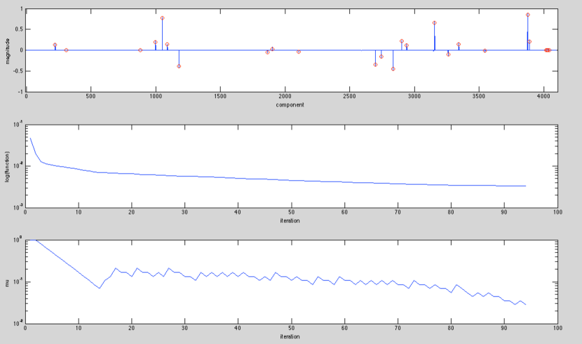
Fig. 1: Results for formulation (58). Top figure shows spikes in true signal (bars) and recovered spikes (circles), showing accurate recovery of the true signal. Middle figure shows the function values at each iteration, while the bottom figure shows the values of $\mu_{k}$ at each iteration $k$.

Consider now the linear least-squares problem with a component-wise MCP regularized $\phi(\cdot)$ defined in (19):

$$\min_{x}\,\frac{1}{2}\|Ax-b\|_{2}^{2}+\nu\sum_{i=1}^{n}\phi(x_{i}),$$ (59)

where $\nu>0$ is again the regularization parameter. In replacing the regularizer $\|\cdot\|_{1}$ of (58) with the nonconvex regularizer of (59), we reduce bias in the solution at the cost of introducing nonconvexity and thus the possibility of local minima.

To test ProxDescent on this problem, we used a different random instance of the same problem as in (58), with the same parameter settings. We define the parameters of the MCP regularizer (19) to be $\lambda=1$ and $a=\|\hat{x}\|_{\infty}/3$. These choices ensure that the MCP function has similar slope to $\|\cdot\|_{1}$ near zero and that it achieves its maximum value of $a\lambda^{2}/2$ for the larger spikes. Results are shown in Figure 2, using the same format as Figure 1 for the subfigures. Despite the nonconvexity, ProxDescent appears to have no trouble finding the global minimum of (59), and in a similar number of iterations as for (58) ($84$, in this particular instance). In fact, a close comparison of the top subfigures in Figures 1 and 2 indicates that the recovered spikes in Figures 1 have slightly lower magnitudes in general than the true spikes, an effect that is not present in Figure 2. This effect is subtle for the choice of $\nu$ used here (detectable only in high-precision versions of the plots), but it illustrates nicely the unbiasedness property of the MCP regularizer. Once again, we see a faint downward trend in the value of $\mu_{k}$, and a convergence rate that is clearly linear, until the solution is identified to high accuracy at about iteration 80.

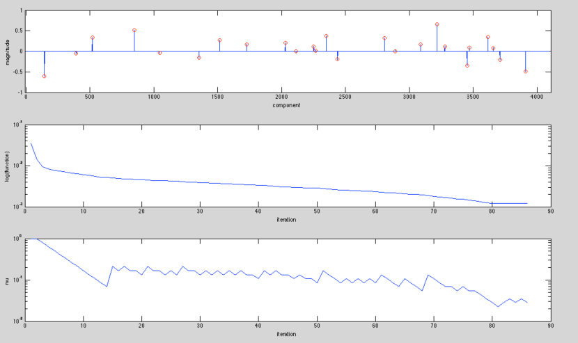
Fig. 2: Results for formulation (59). Top figure shows spikes in true signal (bars) and recovered spikes (circles), showing accurate recovery of the true signal. Middle figure shows the function values at each iteration, while the bottom figure shows the values of $\mu_{k}$ at each iteration $k$.

Finally, we consider the following nonlinear optimization problem:

$$\min\,p^{T}x\;\;\mbox{subject to}\;\;c(x)=0,\;\;\underline{x}\leq x\leq\overline{x},$$ (60)

where $c:\Re^{n}\to\Re^{q}$ is a smooth nonlinear vector function. A nonsmooth penalty formulation of this problem, stated in a form consistent with (1), is as follows:

$$\min\,p^{T}x+\nu\|c(x)\|_{1}+I_{[\underline{x},\overline{x}]}(x),$$ (61)

where the indicator function $I_{[\underline{x},\overline{x}]}(x)$ takes the value $0$ if the bound constraints $\underline{x}\leq x\leq\overline{x}$ are satisfied, and $\infty$ otherwise. This problem was considered in [26], where a sequential $\ell_{1}$-linear programming algorithm was proposed to solve it. When ProxDescent is applied to (61), the only essential difference between it and the algorithm of [26] is that the latter uses an $\ell_{\infty}$ (“box-shaped”) trust region on the step $d$ in its subproblem, in place of the quadratic prox-term $(\mu/2)|d|^{2}$ of (3), which is equivalent to an $\ell_{2}$-norm (circular) trust region. (In fact, the code used to obtain numerical results in [26] was easily modified to produce the results shown here.)

We use ProxDescent on the framework (61) to solve two problems from [26], arising from the restoration of stable operation of a power grid following a disruption, such as loss of a transmission line. In this application, the variables $x$ represent voltage phasors at each node of the grid and various slacks in the formulation, while $c(x)$ is derived from the (nonlinear) model of AC power flow. The bounds on $x$ represent acceptable deviations of voltage magnitude from $1$, and acceptable values of the amount of load to be shed from the nodes of the grid. The first problem is of a type that commonly arises in the power grid application, where the number of constraints active at the solution of (60) equals the number of variables, so that methods that use linearization of the constraints (including ProxDescent and the algorithm of [26]) reduce to Newton’s method on the system of nonlinear equations represented by the active constraints, and rapid convergence is observed once the active set has been determined correctly. In the second problem, the number of active constraints is fewer than the number of variables, so rapid convergence cannot be expected from a first-order method. Here, as in [26], convergence is considerably slower.

For both datasets, we set $\tau=1.5$, $\sigma=10^{-3}$, and $\mu_{\mbox{\scriptsize\rm min}}=10^{-3}$ in ProxDescent, and terminate when the relative change in objective falls below $10^{-5}$. Results for the first problem are shown in Figure 3. This problem has $143$ variables and $143$ active constraints at the solution. Convergence occurred in $26$ iterations, with a total of $44$ subproblems solved. In Figure 3, we consider separately the contributions from the $p^{T}x$ term and the penalty term $\|c(x)\|_{1}$. Both exhibit steady linear convergence to their optimal values. Two subproblems are solved on most iterations, because we try to decrease the value of $\mu$ then increase it again when the smaller value fails to satisfy the sufficient decrease test. Note that $\mu_{k}$ stabilizes at $.058$ on later iterations. Less than one second of execution time was required on a MacBook Pro (2 GHz Intel i7 with 8GB RAM), using Matlab, the MATPOWER package [55] for modeling and solving power grid problems, and CPLEX. The number of major iterations required was similar to the S$\ell_{1}$LP algorithm described in [26]. We also coded a version of the algorithm that attempts to determine the set of active constraints manually once the active set appears to have settled down, solving a system of nonlinear equations based on the KKT conditions and making small heuristic adjustments to the active set in search of a stationary point. This version takes 21 iterations, and about half the run time.

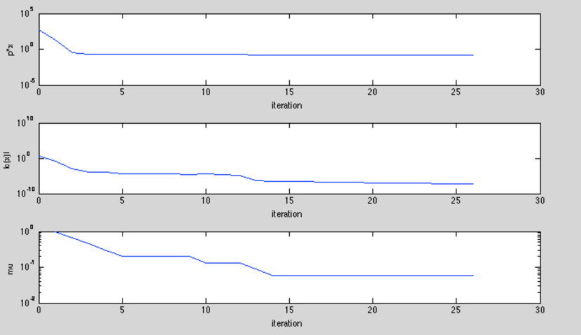
Fig. 3: Results for formulation (61), derived from a 57-bus power grid in which the number of active constraints at the solution equals the number of variables. Top figure shows $p^{T}x_{k}$ plotted against iteration $k$; middle figure show $\|c(x_{k})\|_{1}$; bottom figure shows $\mu_{k}$.

The second data set for (61) is derived from a 118-bus system, and has 262 variables, and 260 constraints active at the solution. Convergence behavior is quite similar to the first case, featuring Q-linear convergence at a rate of about $.5$ for the constraint violation measure $\|c(x_{k})\|_{1}$. $\mu_{k}$ stabilizes at the same value $.058$ as for the first data set, and convergence is declared after $21$ iterations, with $34$ subproblems solved, in about $.6$ seconds of CPU time. An active-set version of the approach requires only $11$ iterations and about $.18$ seconds of CPU time.

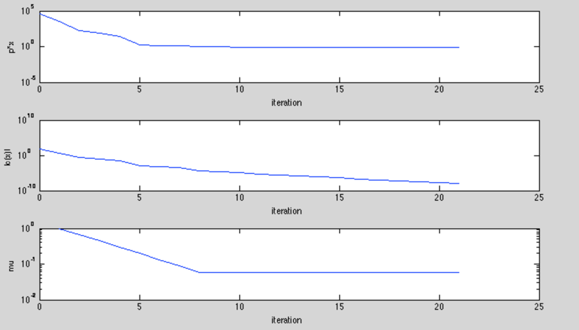
Fig. 4: Results for formulation (61), derived from a 118-bus power grid in which the number of active constraints at the solution is smaller than the number of variables. Top figure shows $p^{T}x_{k}$ plotted against iteration $k$; middle figure show $\|c(x_{k})\|_{1}$; bottom figure shows $\mu_{k}$.

Standard theory

The basic building block for variational analysis (see Rockafellar and Wets [40] or Mordukhovich [35]) is the normal cone to a (locally) closed set $S$ at a point $s\in S$, denoted by $N_{S}(s)$. It consists of all normal vectors: limits of sequences of vectors of the form $\lambda(u-v)$ for points $u,v\in\Re^{m}$ approaching $s$ such that $v$ is a closest point to $u$ in $S$, and scalars $\lambda>0$. On the other hand, tangent vectors are limits of sequences of vectors of the form $\lambda(u-s)$ for points $u\in S$ approaching $s$ and scalars $\lambda>0$. The set $S$ is Clarke regular at $s$ when the inner product of any normal vector with any tangent vector is always nonpositive. Closed convex sets and smooth manifolds are everywhere Clarke regular.

The epigraph of a function $h:\Re^{m}\to\bar{\Re}$ is the set

$$\mbox{epi}\,h~{}=~{}\{(c,r)\in\Re^{m}\times\Re:r\geq h(c)\}.$$

If the value of $h$ is finite at some point $\bar{c}\in\Re^{m}$, then $h$ is lower semicontinuous nearby if and only if its epigraph is locally closed around the point $\big{(}\bar{c},h(\bar{c})\big{)}$. Henceforth we focus on that case.

The subdifferential of $h$ at $\bar{c}$ is the set

$$\partial h(\bar{c})~{}=~{}\big{\{}v\in\Re^{m}\,:\,(v,-1)\in N_{\mbox{\scriptsize\mbox{epi}}\,h}(\bar{c},h\big{(}\bar{c})\big{)}\big{\}}$$

and the horizon subdifferential is

$$\partial^{\infty}h(\bar{c})~{}=~{}\big{\{}v\in\Re^{m}:(v,0)\in N_{\mbox{\scriptsize\mbox{epi}}\,h}\big{(}\bar{c},h(\bar{c})\big{)}\big{\}}$$ (62)

(see [40, Theorem 8.9]). The function $h$ is subdifferentially regular at $\bar{c}$ if its epigraph is Clarke regular at $\big{(}\bar{c},h(\bar{c})\big{)}$ (as holds in particular if $h$ is convex lower semicontinuous, or smooth). Subdifferential regularity implies that $\partial h(\bar{c})$ is a closed and convex set in $\Re^{m}$, and its recession cone is exactly $\partial^{\infty}h(\bar{c})$ (see [40, Corollary 8.11]). In the case when $h$ is locally Lipschitz, it is almost everywhere differentiable: $h$ is then subdifferentially regular at $\bar{c}$ if and only if its directional derivative for every direction $d\in\Re^{m}$ equals

$$\limsup_{c\to\bar{c}}\mbox{$\langle\nabla h(c),d\rangle$},$$

where the $\limsup$ is taken over points $c$ where $h$ is differentiable.

Consider a subgradient $\bar{v}\in\partial h(\bar{c})$, and a localization of the subdifferential mapping $\partial h$ around the point $(\bar{c},\bar{v})$, by which we mean a set-valued mapping $T\colon\Re^{m}\;{\lower 1.0pt\hbox{$\rightarrow$}}\kern-10.0pt\hbox{\raise 2.8pt\hbox{$\rightarrow$}}\;\Re^{m}$ defined by

$$T(y)=\left\{\begin{array}[]{ll}\partial h(y)\cap B_{\epsilon}(\bar{v})&(|y-\bar{c}|\leq\epsilon,~{}|h(y)-h(\bar{c})|\leq\epsilon)\\ \emptyset&(\mbox{otherwise})\end{array}\right.$$

for some constant $\epsilon>0$. The function $h$ is prox-regular at $\bar{c}$ for $\bar{v}$ if some such localization is hypomonotone: that is, for some constant $\rho>0$, we have

$$z\in T(y)~{}\mbox{and}~{}z^{\prime}\in T(y^{\prime})~{}~{}\Rightarrow~{}~{}\mbox{$\langle z^{\prime}-z,y^{\prime}-y\rangle$}\geq-\rho|y^{\prime}-y|^{2}.$$

This definition is equivalent to Definition 1 (with the same constant $\rho$) [40, Example 12.28 and Theorem 13.36]. Prox-regularity at $\bar{c}$ (for all subgradients $v$) implies subdifferential regularity.

A general class of prox-regular functions common in engineering applications is “lower ${\cal C}^{2}$” functions [40, Definition 10.29]. A function $h:\Re^{m}\to\Re$ is lower ${\cal C}^{2}$ around a point $\bar{c}\in\Re^{m}$ if $h$ has the local representation

$$h(c)=\max_{t\in T}f(c,t)~{}~{}\mbox{for}~{}c\in\Re^{m}~{}\mbox{near}~{}\bar{c},$$

for some function $f:\Re^{m}\times T\to\Re$, where the space $T$ is compact and the quantities $f(c,t)$, $\nabla_{c}f(c,t)$, and $\nabla^{2}_{cc}f(c,t)$ all depend continuously on $(c,t)$. All lower ${\cal C}^{2}$ functions are prox-regular [40, Proposition 13.3]. A simple equivalent property, useful in theory though harder to check in practice, is that $h$ has the form $g-\kappa|\cdot|^{2}$ around the point $\bar{c}$ for some continuous convex function $g$ and some constant $\kappa$.

The normal cone is crucial to the definition of another central variational-analytic tool. Given a set-valued mapping $F:\Re^{p}\;{\lower 1.0pt\hbox{$\rightarrow$}}\kern-10.0pt\hbox{\raise 2.8pt\hbox{$\rightarrow$}}\;\Re^{q}$ with closed graph,

$$\mbox{gph}\,F=\{(u,v):v\in F(v)\},$$

at any point $(\bar{u},\bar{v})\in\mbox{gph}\,F$, the coderivative $D^{*}F(\bar{u}|\bar{v}):\Re^{q}\;{\lower 1.0pt\hbox{$\rightarrow$}}\kern-10.0pt\hbox{\raise 2.8pt\hbox{$\rightarrow$}}\;\Re^{p}$ is defined by

$$w\in D^{*}F(\bar{u}|\bar{v})(y)~{}\Leftrightarrow~{}(w,-y)\in N_{\mbox{\scriptsize gph}\,F}(\bar{u},\bar{v}).$$

The coderivative generalizes the adjoint of the derivative of smooth vector function: for smooth $c:\Re^{n}\to\Re^{m}$, the set-valued mapping $x\mapsto F(x):=\{c(x)\}$ has coderivative given by $D^{*}F(x|c(x))(y)=\{\nabla c(x)^{*}y\}$ for all $x\in\Re^{n}$ and $y\in\Re^{m}$. As we see next, coderivative calculations drive two of the arguments in Section 4.1.

Proof of Corollary 5

Corresponding to any linear map $A\colon\Re^{p}\rightarrow\Re^{q}$, define a set-valued mapping $F_{A}\colon\Re^{p}\;{\lower 1.0pt\hbox{$\rightarrow$}}\kern-10.0pt\hbox{\raise 2.8pt\hbox{$\rightarrow$}}\;\Re^{q}$ by $F_{A}(u)=Au-S$. A coderivative calculation shows, for vectors $v\in\Re^{p}$,

$$D^{*}F_{A}(0|0)(v)=\left\{\begin{array}[]{ll}\{A^{*}v\}&\big{(}v\in N_{S}(0)\big{)}\\ \emptyset&(\mbox{otherwise}).\end{array}\right.$$

Hence, by assumption, the only vector $v\in\Re^{p}$ satisfying $0\in D^{*}F_{\bar{A}}(0|0)(v)$ is zero, so by [40, Thm 9.43], the mapping $F_{\bar{A}}$ is metrically regular at zero for zero. Applying Theorem 4 shows that there exist constants $\delta,\gamma>0$ such that, if $\|A-\bar{A}\|<\delta$ and $|v|<\delta$, then we have

$$\mbox{\rm dist}\,\!\big{(}0,F_{A}^{-1}(-v)\big{)}\leq\gamma\,\mbox{\rm dist}\,\!\big{(}-v,F_{A}(0)\big{)},$$

or equivalently,

$$\mbox{\rm dist}\,\!\big{(}0,A^{-1}(S-v)\big{)}\leq\gamma\,\mbox{\rm dist}\,(v,S).$$

Since $0\in S$, the right-hand side is bounded above by $\gamma|v|$, so the result follows.     $\Box$

Proof of Corollary 6

We simply need to check that the set-valued mapping $G\colon\Re^{p}\;{\lower 1.0pt\hbox{$\rightarrow$}}\kern-10.0pt\hbox{\raise 2.8pt\hbox{$\rightarrow$}}\;\Re^{q}$ defined by $G(z)=F(z)-S$ is metrically regular $\bar{z}$ for zero. Much the same coderivative calculation as in the proof of Corollary 5 shows, for vectors $v\in\Re^{p}$, the formula

$$D^{*}G(\bar{z}|0)(v)=\left\{\begin{array}[]{ll}\{\nabla F(\bar{z})^{*}v\}&\big{(}v\in N_{S}(\bar{z})\big{)}\\ \emptyset&(\mbox{otherwise}).\end{array}\right.$$

Hence, by assumption, the only vector $v\in\Re^{p}$ satisfying $0\in D^{*}G(\bar{z}|0)(v)$ is zero, so metric regularity follows by [40, Thm 9.43].     $\Box$

Alternative proof of Theorem 4

In the text we gave a short ad hoc proof of Theorem 4. Here we present a more formal approach. Denote the space of linear maps from $\Re^{p}$ to $\Re^{q}$ by $L(\Re^{p},\Re^{q})$, and define a mapping $g\colon L(\Re^{p},\Re^{q})\times\Re^{p}\to\Re^{q}$ and a parametric mapping $g_{H}\colon\Re^{p}\to\Re^{q}$ by $g(H,u)=g_{H}(u)=Hu$ for maps $H\in L(\Re^{p},\Re^{q})$ and points $u\in\Re^{p}$. Using the notation of [14, Section 3], the Lipschitz constant $l[g](0;\bar{u},0)$, is by definition the infimum of the constants $\rho$ for which the inequality

$$d\big{(}w,g_{H}(u)\big{)}\leq\rho d\big{(}u,g_{H}^{-1}(w)\big{)}$$ (63)

holds for all triples $(u,w,H)$ sufficiently near the triple $(\bar{u},0,0)$. Inequality (63) says simply

$$|w-Hu|\leq\rho|u-z|~{}~{}\mbox{for all $z\in\Re^{p}$ satisfying $Hz=w$},$$

a property that holds providing $\rho\geq\|H\|$. We deduce

$$l[g](0;\bar{u},0)=0.$$ (64)

We can also consider $F+g$ as a set-valued mapping from $L(\Re^{p},\Re^{q})\times\Re^{p}$ to $\Re^{q}$, defined by $(F+g)(H,u)=F(u)+Hu$, and then the parametric mapping $(F+g)_{H}\colon\Re^{p}\;{\lower 1.0pt\hbox{$\rightarrow$}}\kern-10.0pt\hbox{\raise 2.8pt\hbox{$\rightarrow$}}\;\Re^{q}$ is defined in the obvious way: in other words, $(F+g)_{H}(u)=F(u)+Hu$. According to [14, Theorem 2], equation (64) implies the following relationship between the “covering rates” for $F$ and $F+g$:

$$r[F+g](0;\bar{u},\bar{v})=r[F](\bar{u},\bar{v}).$$

The reciprocal of the right-hand side is, by definition, the infimum of the constants $\kappa>0$ such that inequality (23) holds for all pairs $(u,v)$ sufficiently near the pair $(\bar{u},\bar{v})$. By metric regularity, this number is strictly positive. On the other hand, the reciprocal of the left-hand side is, by definition, the infimum of the constants $\gamma>0$ such that inequality (24) holds for all triples $(u,v,H)$ sufficiently near the pair $(\bar{u},\bar{v},0)$.

References

- [1] J. Bolte, A. Daniilidis, and A. S. Lewis, Generic optimality conditions for semialgebraic convex problems, Mathematics of Operations Research, 36 (2011), pp. 55–70.
- [2] J. F. Bonnans and A. Shapiro, Perturbation Analysis of Optimization Problems, Springer Series in Operations Research, Springer, 2000.
- [3] J. V. Burke, Descent methods for composite nondifferentiable optimization problems., Mathematical Programming, Series A, 33 (1985), pp. 260–279.
- [4] , On the identification of active constraints II: The nonconvex case, SIAM Journal on Numerical Analysis, 27 (1990), pp. 1081–1102.
- [5] J. V. Burke and J. J. Moré, On the identification of active constraints, SIAM Journal on Numerical Analysis, 25 (1988), pp. 1197–1211.
- [6] R. Byrd, N. I. M. Gould, J. Nocedal, and R. A. Waltz, On the convergence of successive linear-quadratic programming algorithms, SIAM Journal on Optimization, 16 (2005), pp. 471–489.
- [7] J.-F. Cai, E. Candès, and Z. Shen, A singular value thresholding algorithm for matrix completion, SIAM Journal on Optimization, 20 (2010), pp. 1956–1982.
- [8] E. Candès and B. Recht, Exact matrix completion via convex optimization, Foundations of Computational Mathematics, 9 (2009), pp. 717–772.
- [9] E. J. Candès, Compressive sampling, in Proceedings of the International Congress of Mathematicians, Madrid, 2006.
- [10] S. S. Chen, D. L. Donoho, and M. A. Saunders, Atomic decomposition by basis pursuit, SIAM Journal on Scientific Computing, 20 (1998), pp. 33–61.
- [11] P. Combettes and T. Pennanen, Proximal methods for cohypomonotone operators, SIAM Journal on Control and Optimization, 43 (2004), pp. 731–742.
- [12] P. L. Combettes and V. R. Wajs, Signal recovery by proximal forward-backward splitting, Multiscale Modeling and Simulation, 4 (2005), pp. 1168–1200.
- [13] A. Daniilidis, W. Hare, and J. Malick, Geometrical interpretation of the proximal-type algorithms in structured optimization problems, Optimization, 55 (2006).
- [14] A. V. Dmitruk and A. Y. Kruger, Metric regularity and systems of generalized equations, Journal of Mathematical Analysis and Applications, 342 (2008), pp. 864–873.
- [15] A. L. Dontchev, A. S. Lewis, and R. T. Rockafellar, The radius of metric regularity, Transactions of the American Mathematical Society, 355 (2003), pp. 493–517.
- [16] B. Efron, T. Hastie, I. Johnstone, and R. Tibshirani, Least angle regression, Annals of Statistics, 32 (2004), pp. 407–499.
- [17] J. Fan and R. Li, Variable selection via nonconvex penalized likelihood and its oracle properties, Journal of the American Statistical Association, 96 (2001), pp. 1348–1361.
- [18] R. Fletcher and E. Sainz de la Maza, Nonlinear programming and nonsmooth optimization by successive linear programming, Mathematical Programming, 43 (1989), pp. 235–256.
- [19] M. P. Friedlander, N. I. M. Gould, S. Leyffer, and T. S. Munson, A filter active-set trust-region method, Preprint ANL/MCS-P1456-0907, Mathematics and Computer Science Division, Argonne National Laboratory, 9700 S. Cass Avenue, Argonne IL 60439, September 2007.
- [20] M. Fukushima and H. Mine, A generalized proximal point algorithm for certain nonconvex minimization problems, International Journal of Systems Science, 12 (1981), pp. 989–1000.
- [21] E. T. Hale, W. Yin, and Y. Zhang, A fixed-point continuation method for -minimization: Methodology and convergence, SIAM Journal on Optimization, 19 (2008), pp. 1107–1130.
- [22] W. Hare and A. Lewis, Identifying active constraints via partial smoothness and prox-regularity, Journal of Convex Analysis, 11 (2004), pp. 251–266.
- [23] A. Iusem, T. Pennanen, and B. Svaiter, Inexact variants of the proximal point algorithm without monotonicity, SIAM Journal on Optimization, 13 (2003), pp. 1080–1097.
- [24] S. Jokar and M. E. Pfetsch, Exact and approximate sparse solutions of underdetermined linear equations, SIAM Journal on Scientific Computing, 31 (2008), pp. 23–44.
- [25] A. Kaplan and R. Tichatschke, Proximal point methods and nonconvex optimization, Journal of Global Optimization, 13 (1998), pp. 389–406.
- [26] T. Kim and S. J. Wright, An SLP-active set approach for feasibility restoration in power systems, tech. report, Computer Science Department, University of Wisconsin-Madison, May 2014. arXiv:1405.0322.
- [27] G. Lan, Bundle-level type methods uniformly optimal for smooth and nonsmooth convex optimization, Mathematical Programming, Series A, 149 (2015), pp. 1–45.
- [28] C. Lemaréchal, F. Oustry, and C. Sagastizábal, The -Lagrangian of a convex function, Transactions of the American Mathematical Society, 352 (2000), pp. 711–729.
- [29] A. Levy, Lipschitzian multifunctions and a Lipschitzian inverse mapping theorem, Mathematics of Operations Research, 26 (2001), pp. 105–118.
- [30] A. Lewis, Active sets, nonsmoothness, and sensitivity, SIAM Journal on Optimization, 13 (2003), pp. 702–725.
- [31] O. L. Mangasarian, Minimum-support solutions of polyhedral concave programs, Optimization, 45 (1999), pp. 149–162.
- [32] B. Martinet, Régularisation d’inéquations variationnelles par approximations successives, Rev. Française Informat. Recherche Opérationnelle, 4 (1970), pp. 154–158.
- [33] R. Mifflin and C. Sagastizábal, A VU-algorithm for convex minimization, Mathematical Programming, Series B, 104 (2005), pp. 583–608.
- [34] S. A. Miller and J. Malick, Newton methods for nonsmooth convex minimization: Connections among -Lagrangian, Reimannian Newton, and SQP methods, Mathematical Programming, Series B, 104 (2005), pp. 609–633.
- [35] B. Mordukhovich, Variational Analysis and Generalized Differentiation, I: Basic Theory; II: Applications, Springer, New York, 2006.
- [36] T. Pennanen, Local convergence of the proximal point algorithm and multiplier methods without monotonicity, Mathematics of Operations Research, 27 (2002), pp. 170–191.
- [37] B. Recht, M. Fazel, and P. Parrilo, Guaranteed minimum-rank solutions of matrix equations via nuclear norm minimization, SIAM Review, 52 (2010), pp. 471–501.
- [38] R. Rockafellar, Monotone operators and the proximal point algorithm, SIAM Journal on Control and Optimization, 14 (1976), pp. 877–898.
- [39] R. T. Rockafellar, Convex Analysis, Princeton University Press, Princeton, N.J., 1970.
- [40] R. T. Rockafellar and R. J. Wets, Variational Analysis, Springer, 1998.
- [41] L. Rudin, S. Osher, and E. Fatemi, Nonlinear total variation based noise removal algorithms, Physica D, 60 (1992), pp. 259–268.
- [42] C. Sagastizábal, Composite proximal bundle method, Mathematical Programming, Series B, 140 (2013), pp. 189–233.
- [43] C. Sagastizábal and R. Mifflin, Proximal points are on the fast track, Journal of Convex Analysis, 9 (2002), pp. 563–579.
- [44] A. Shapiro, On a class of nonsmooth composite functions, Mathematics of Operations Research, 28 (2003), pp. 677–692.
- [45] W. Shi, G. Wahba, S. J. Wright, K. Lee, R. Klein, and B. Klein, LASSO-Patternsearch algorithm with application to opthalmology data, Statistics and its Interface, 1 (2008), pp. 137–153.
- [46] J. Spingarn, Submonotone mappings and the proximal point algorithm, Numerical Functional Analysis and Optimization, 4 (1981/82), pp. 123–150.
- [47] R. Tibshirani, Regression shrinkage and selection via the LASSO, Journal of the Royal Statistical Society B, 58 (1996), pp. 267–288.
- [48] Z. Wen, W. Yin, H. Zhang, and D. Goldfarb, On the convergence of an active set method for minimization, SIAM Journal of Scientific Computing, 32 (2010), pp. 1832–1857.
- [49] S. J. Wright, Convergence of an inexact algorithm for composite nonsmooth optimization, IMA Journal of Numerical Analysis, 9 (1990), pp. 299–321.
- [50] , Identifiable surfaces in constrained optimization, SIAM J. Control Optim., 31 (1993), pp. 1063–1079.
- [51] S. J. Wright, R. D. Nowak, and M. A. T. Figueiredo, Sparse reconstruction by separable approximation, IEEE Transactions on Signal Processing, 57 (2009), pp. 2479–2493.
- [52] Y. Yuan, Conditions for convergence of a trust-region method for nonsmooth optimization, Mathematical Programming, 31 (1985), pp. 220–228.
- [53] , On the superlinear convergence of a trust region algorithm for nonsmooth optimization, Mathematical Programming, 31 (1985), pp. 269–285.
- [54] C. H. Zhang, Nearly unbiased variable selection under minimax concave penalty, Annals of Statistics, 38 (2010), pp. 894–942.
- [55] R. D. Zimmerman, C. E. Murillo-Sánchez, and R. J. Thomas, MATPOWER: Steady-state operations, planning, and analysis tools for power systems research and education, IEEE Transactions on Power Systems, 26 (2011), pp. 12–19.