Photonic Feshbach Resonance

Hermann Feshbach predicted fifty years ago feshbach58 that when two atomic nuclei are scattered within an open entrance channel— the state observable at infinity, they may enter an intermediate closed channel — the locally bounded state of the nuclei. If the energy of a bound state of in the closed channel is fine-tuned to match the relative kinetic energy, then the open channel and the closed channel “resonate”, so that the scattering length becomes divergent pethick02 . We find that this so-called Feshbach resonance phenomenon not only exists during the collisions of massive particles, but also emerges during the coherent transport of massless particles, that is, photons confined in the coupled resonator arrays lzhou08 . We implement the open and the closed channels inside a pair of such arrays, linked by a separated cavity or a tunable qubit. When a single photon is bounded inside the closed channel by setting the relevant physical parameters appropriately, the vanishing transmission appears to display this photonic Feshbach resonance. The general construction can be implemented through various experimentally feasible solid state systems, such as the couple defected cavities in photonic crystals. The numerical simulation based on finite-different time-domain(FDTD) method confirms our conceive about physical implementation.

The phenomenon of Feshbach resonance has been found in many physical systems over the years, such as the electron scattering of atoms schulz73a and diatomic molecules schulz73b . More recently, the development of laser cooling technologies has enabled the observation of low-energy Feshbach resonance in ultra-cold atoms courteille98 ; roberts98 ; vuletic99 and Bose-Einstein condensates (BEC) ketterle98 ; timmermans99 . These experiments have helped verify the simulation of various theoretical predictions of condensing phenomena in solid state systems dsjin08rev . The latter in particular exemplifies the resonance phenomenon as a means for adjusting inter-atomic coupling in realizing various quantum phases ranging from BEC to BCS d.s.jin02 ; d.s.jin08 .

On the other hand, since their first discovery by von Neumann and Wigner neumann29 , bound states have been studied in a general continuum friedrich85 and the emergence of a bounded energy level has been verified by various models lee54 ; fano61 ; anderson61 , extracting from the simple coupling of a discrete level with a continuum. Quasi-bound states have been predicted in tight-binding fermionic quantum wires nakamura07 for localized fermions and in the optical coupled resonator arrays lzhou08 ; hdong08 ; zrgong08 for confined photons. It has also found various applications in many quantum optical devices fan05 ; fan05_optic ; fan07 , including the single-photon transistor lukin07 . Under this retrospect, we ask if it is possible to control exactly when the photons become bounded and unbounded through an external parameter, viz. to implement an optical version of Feshbach resonance.

The desired resonance between the bound and the unbound states can be found inside a pair of parallelly placed coupled resonator arrays lzhou08 , a series of consecutively placed optical microcavities that entrap photons and allow photon-hopping from one of the cavities to its closest neighbors at left and right. The two arrays are connected by a central cavity that acts as a quantum controller and couples separately to one cavity in each of the arrays, as shown in Fig. 1(a), forming an H-shape system. We designate the upper array as array A with the Hamiltonian

$$H=\omega_{\mathrm{A}}\sum_{j}a_{j}^{\dagger}a_{j}+(J_{\mathrm{A}}\sum_{j}a_{j}^{\dagger}a_{j+1}+g_{\mathrm{A}}a_{0}c^{\dagger}+\mathrm{h.c}),$$ (1)

where the second summation describes the tight-binding hopping of photons between neighboring cavities with hopping coefficient $J_{\mathrm{A}}$ while the first one accounts for the static photon occupations in the cavities. $a_{j}$ denotes the annihilation operator of the bosonic mode for the $j$-th cavity field and we assume that the mode frequency $\omega_{\mathrm{A}}$ of each cavity field is identical. The last term is the interaction between the central cavity $C$ of single mode frequency $\Omega$ and the zeroth resonator of array A with coupling strength $g_{\mathrm{A}}$. $c$ is corresponding annihilation bosonic operator for central cavity. The lower array is designated as array B, the Hamiltonian $H_{\mathrm{B}}$ for which is no different from Eq. (1) except the change of the bosonic mode operator to $b_{j}$,the hopping coefficient to $J_{\mathrm{B}}$, the mode frequency to $\omega_{\mathrm{B}}$ and the coupling strength to $g_{\text{B}}$. Then,the total model Hamiltonian reads $H=H_{\mathrm{A}}+H_{\mathrm{B}}+\Omega c^{\dagger}c.$

One experimental available system of the model is based on photonic crystal, which will be described in details below. We have to point out that there is a drawback in our setup: the inter-cavity coupling cannot be externally manipulated, once the photonic-crystal based metamaterial is fabricated as an all-optical chip. However, for single photon transferring, the role of central cavity as that of a qubit with two levels $\left|e\right\rangle=\left|1\right\rangle$ and $\left|g\right\rangle=$ $\left|0\right\rangle$, corresponding to the single photon state and vacuum of the central cavity. This identification motivates us to use a qubit controller replacing the central cavity equivalently in the single photon case. Therefore, the phenomenon predicted here can be realized in the hybrid system of photonic crystal and quantum dots with external controllable parameter. Our general construction can also be implemented through the circuit QED system wallraff04 including two coupled superconducting transmission line cavity linked by charge or flux qbit. The replacement of the central cavity by a controllable qubit can overcome the drawback mentioned above.

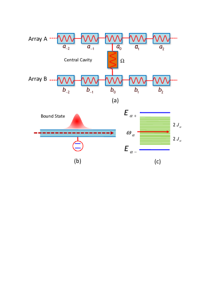
Figure 1: The photonic Feshbach resonance based on the coupled resonator arrays: (a) schematic of the H-shape system consisting of two coupled resonator arrays, array A and array B, connected by a qubit controller of level spacing $\Omega$. Each of the cavity in the two arrays is characterized by the cavity field mode it confines and hereby indicated by the bosonic operator $a_{j}$ or $b_{j}$ and indexed by the relative distance $j$ from the zeroth cavity with which the qubit controller couples; (b) probability distribution of a single photon in a coupled resonator array for a quasi-bound state. When the level spacing $\Omega$ of the qubit controller matches certain values, the probability amplitude would vanish at the two ends of the array; (c) the energy state distribution for array $\alpha$, $\alpha\in\left\{A,B\right\}$, relative to the common eigenfrequency $\omega_{\alpha}$ of the cavity fields: a pair of a continuum and a discrete level above and below $\omega_{\alpha}$.

In the following , we use the Jaynes-Cummings couplings $g_{\alpha}c^{\dagger}\left|g\right\rangle\left\langle e\right|+\mathrm{h.c}$ ($\alpha=A,B$) to modeling the central cavity couplings in the single photon case. The Hilbert space is spanned by the tensor product $\left\{\left|e\right\rangle,\left|g\right\rangle\right\}\bigotimes_{j}\left|n_{\mathrm{A},j}\right\rangle\bigotimes_{j}\left|n_{\mathrm{B},j}\right\rangle$ where $\left|n_{\alpha,j}\right\rangle$ denotes the state of array $\alpha$ with its $j$-th cavity being occupied with $n_{\alpha,j}$ number of photons. When separated from the other and studied individually, each coupled resonator array is described by the subsystem Hamiltonian $H_{\alpha}$ and possesses two bound states, reminiscent that of the Feshbach resonance. The states are the particular superposition of eigenstates for the Hamiltonian $H_{\alpha}$, comprised by a subset of the basis vectors described above. For array A, the state is namely $\left|\varphi_{\mathrm{A}}\right\rangle=\sum_{j}u_{\mathrm{A},g}(j)\left|g,1_{j},0\right\rangle+u_{\mathrm{A},e}\left|e,0,0\right\rangle$ where only the excited state of the central cavity and a single-photon excitation in one of the cavities, as indicated by the $1_{j}$ symbol, are included. The coefficients $u_{\mathrm{A},g}(j)$ and $u_{\mathrm{A},e}$ in the equation constitute the spectrum of probability distributions of these states. That of array B takes a similar form with amplitudes $u_{\mathrm{B},g}(j)$ and $u_{\mathrm{B},e}$.

To see whether there are bounded single-photon states within their individual coupled resonator array, we can solve the discrete-coordinate scattering equation associated with their corresponding eigenvalue $E$ for the probability spectrum,

$$[E-\omega_{\alpha}-V_{\alpha}(E)]u_{\alpha,g}(j)=-J_{\alpha}[u_{\alpha,g}(j+1)+u_{\alpha,g}(j-1)]$$ (2)

where the term $V_{\alpha}(E)=g_{\alpha}^{2}\delta_{j0}/(E-\Omega)$ on the left hand side is contributed by the JC type interaction between the central cavity and the coupled resonator array. $V_{\alpha}(E)$ is a resonate potential that depends on the eigenenergy $E$. In the continuous limit of the coordinate $j\rightarrow x$, this term reduces to a $\delta$ -type potential

$$V_{\alpha}(E,x)=\frac{g_{\alpha}^{2}}{E-\Omega}\delta(x).$$ (3)

The $\delta$-type potential forms a confining barrier to the transportation of single photon in the coupled resonator array and informs a bounded single photon within, similar to those in the models proposed in Refs. hdong08 ; zrgong08 .

It has a singularity at $E$ being equal to the level spacing $\Omega$, leading to a quasi-plane-wave type solution lzhou08 to Eq. (2), $u_{\alpha,g}(j)=C_{\alpha}\exp(-i\kappa_{\alpha}|j|)$ where $C_{\alpha}$ denotes a constant and the wave number is complex, $\kappa_{\alpha}=\kappa_{\alpha,R}-i\kappa_{\alpha,I}$. The imaginary part $\kappa_{\alpha,I}$ of the wave number can admit a positive value and for the non-zero coupling $g_{\alpha}$, resulting in a decay of the probability distribution of single-photon states over the discrete spatial coordinate $j$. The vanishing probability amplitude towards the ends of the arrays, i.e. along with $|j|\rightarrow\infty$, demonstrates the existence of a bound state of a single photon, as shown in Fig. 1(b). For this system, continuum band has a bandwidth of $4J_{\alpha}$ and their paired discrete levels, denoted respectively by $E_{\alpha+}$ and $E_{\alpha-}$, are gapped from either below or above, as illustrated in Fig. 1(c). Reverted to the conventional language of atomic scattering, the continua of eigenenergies can be considered open channels of multiple admissible energy states in the continuous range $\omega_{\alpha}-2J_{\alpha}<E<\omega_{\alpha}+2J_{\alpha}$. Out of this range, the energy states can only admit two discrete levels that associate with a non-real $k_{\alpha}$, representing closed channels or bound states. These two discrete levels

$$E_{\alpha\pm}=\Omega\pm\frac{g_{\alpha}^{2}}{\sqrt{(E_{\alpha\pm}-\omega_{\alpha})^{2}-4J_{\alpha}^{2}}}.$$ (4)

are exactly solved from the above discrete-coordinate scattering equation. The dependence of these two bound state energies on the various system parameters gives hints to their potential of tunability and controllability. The readers familiar with the approaches by Lee lee54 , Fano fano61 , and Anderson anderson61 shall also find our result here familiar.

The next logical step is to study how the resonance phenomenon arises when two individual arrays are paired to form the H-shape system. The scattering state $\left|\varphi\right\rangle$ of the H-system for single-photon reads $\left|\varphi\right\rangle=\sum_{j}\left[u_{\mathrm{A},g}(j)\left|g,1_{j},0\right\rangle+u_{\mathrm{B},g}(j)\left|g,0,1_{j}\right\rangle\right]+u_{e}\left|e,0,0\right\rangle$. The probability amplitudes $u_{\mathrm{A},g}(j)$ and $u_{\mathrm{B},g}(j)$ of the photonic occupation among the cavities and $u_{e}$ of the atomic excitation in the system can still be analyzed through the time-independent Schrödinger equations, leading to a pair of algebraic scattering equations similar to Eq. (2), one for the probability amplitudes in each array. The distinction of the case here lies in the adding $W_{\alpha}(E)=g_{\alpha}g_{\bar{\alpha}}u_{\bar{\alpha},g}(0))/(E-\Omega)$ in the right hand side with $\alpha$ indexing either A or B. We have used $\bar{\alpha}$ to indicate the dual array relative to $\alpha$; namely, when $\alpha$ indexes A, then $\bar{\alpha}$ indexes B and vice versa. This term reflects a potential again contributed by the interaction of each array with the central cavity. However, because of the coupling between the central cavity and the dual array, additional contribution from the dual array has to be considered.

The set of solutions to the pair of scattering equations are many. The portion we are concerned with are those illustrating a simultaneously existent set of open channel and closed channel in the two coupled resonator arrays. We select one of the particular cases when a single photon is inserted into an open channel in array A from the left for this purpose. The distribution of this single photon in the array is then described by a plane wave, $u_{\mathrm{A}}(j)=\exp(ikj)+r\exp(-ikj)\;(j<0);\;s\exp(ikj)\;(j>0)$. $s$ and $r$ denote, respectively, the transmission and the reflection coefficients of the optical plane wave, indicating the scattering of photon by the effective potential Eq. (3) at the zeroth resonator in the one-dimensional coordinate space. Meanwhile, the distribution amplitude for the single photon in array B can be quasi-plane-wave type, $u_{\mathrm{B}}(j)=C_{\mathrm{B}}\exp\left\{-i\kappa|j|\right\}$, with a complex wave number $\kappa$, and indicate a closed channel, same as that of the individually discussed case. These two distributions in the paired arrays, when combined through the coupled scattering equations, give rise to a unified dual-channel coupling equation

$$(1-s)\sin k\frac{J_{\mathrm{A}}}{g_{\mathrm{A}}}=C_{\mathrm{B}}\sin\kappa\frac{J_{\mathrm{B}}}{g_{\mathrm{B}}}=\frac{g_{\mathrm{A}}s+g_{\mathrm{B}}C_{\mathrm{B}}}{2i(\Omega-E)}.$$ (5)

Therefore, the optical dual-channel resonance occurs when there exists a solution of real $k$ and complex $\kappa$ to Eq. (5) and the eigenenergy $E$ of the photon in array A matches either of the discrete energy levels $E_{\mathrm{B}\pm}$ of array B. The process is illustrated in Fig. 2 for two particular cases with $E$ matching $E_{\mathrm{B}+}$ in Fig. 2 (a) or $E_{\mathrm{B}-}$ in Fig. 2(b). The two possibilities of channel resonances is further illustrated in Fig. 2 (c) with the equivalent potential of array A as a function of the resonator position $j$. The zeroth resonator locates the position of local minimal energy for both the open channels and the closed channel, reflecting the potential barrier set up by the central cavity. The dual-channel resonance occurs as well when the roles of array A and array B are exchanged.

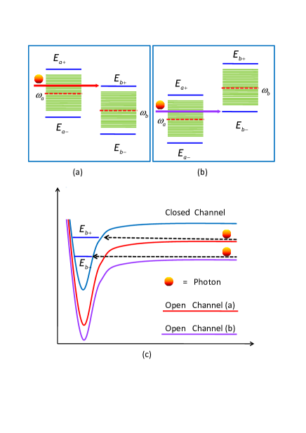
Figure 2: Diagrams of the energy state distributions of the single photon in array A and array B, showing the process of Feshbach resonance between an open channel and a closed channel. Two particular resonance cases exist for an incident photon inserted into array A: (a) the photon energy level in the continuum band in array A is resonant with the upper discrete level $E_{\mathrm{B}+}$ in array B; (b) the photon energy level in the continuum band in array A is resonant with the lower discrete level $E_{\mathrm{B}-}$ in array B. (c) A profile plot illustrating the same two cases of channel resonances relative to the cavity position $j$ the photon occupies.

The criteria of the dual-channel resonance can be met if the transmission coefficient $s$ in Eq. (5) vanishes. This condition implies the circumstance where the incident photon in array A is totally reflected or scattered by the potential barrier set up by the central cavity at position $j=0$. In other words, the level spacing $\Omega$ of the controller becomes our tuning parameter for the photonic Feshbach resonance. Written in terms of the other variables in the dual-channel coupling equation $s=-2iC_{\mathrm{B}}J_{\mathrm{B}}(E-\Omega)\sin\kappa/(g_{\mathrm{A}}g_{\mathrm{B}})-C_{\mathrm{B}}g_{\mathrm{B}}/g_{\mathrm{A}}$, the transmission coefficient vanishes when $E=\Omega-g_{\mathrm{B}}^{2}/(2iJ_{\mathrm{B}}\sin\kappa)$, leading to a complex wave number $\kappa$ as expected. The complete reflection in the open channel can be understood as the divergence effect of s-wave scattering length for the usual Feshbach resonances in three-dimensional space reduced to a version in one-dimensional space. Eliminating the various variables, the transmission coefficient can be expressed as a function of the incident energy $E,i.e.,$

$$s=\begin{cases}F_{\mathrm{A}}(E)\left[F_{\mathrm{A}}(E)-G_{-}(E)\right]^{-1},&E>\omega_{\mathrm{B}}+2J_{\mathrm{B}}\\ F_{\mathrm{A}}(E)\left[F_{\mathrm{A}}(E)-G_{+}(E)\right]^{-1},&E<\omega_{\mathrm{B}}+2J_{\mathrm{B}}\end{cases}$$ (6)

where we have used the shorthands $F_{\alpha}(E)=\sqrt{(E-\omega_{\alpha})^{2}-4J_{\alpha}^{2}}$ with $\alpha\in\left\{\mathrm{A},\mathrm{B}\right\}$ and $G_{\pm}(E)=g_{\mathrm{A}}^{2}F_{\mathrm{B}}(E)/\left((E-\Omega)F_{\mathrm{B}}(E)\pm g_{\mathrm{B}}^{2}\right)$. The norm-squared reflection coefficient $|1-s|^{2}$ is plotted against the photon energy in families of varying level spacing $\Omega$ and coupling constant $g_{A}$ of the qubit controller in Fig. 3. The photon encounters two kinds of characteristic points while propagating through array A. The first one is an indifferentiable turning point where $s=1$ or $E=\omega_{\mathrm{B}}+2J_{\mathrm{B}}$. The potential barrier becomes transparent and the photon is completely transmitted because of the matching coupling between the qubit controller and the dual array B. The second one is the maximum point where the photon is fully reflected when the transmission coefficient is vanishing $s=0$. We hence see the shifting of this peak while $\Omega$ is varied. The reliance on the coupling coefficient $g_{\mathrm{A}}$ determines the width of the peaking.

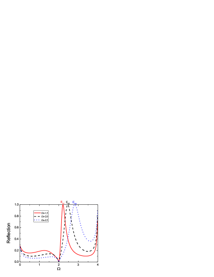
Figure 3: Plots of the norm-squared reflection coefficient $|1-s|^{2}$ against the eigenenergy $E$ of a propagating photon in the coupled resonator array A of the process illustrated in Fig. 2(a). Two tuning parameters are varied: (a) the level spacing $\Omega$ of the qubit controller; and (b) the coupling coefficient $g_{\mathrm{A}}$ between the qubit controller and the zeroth cavity in array A. Other parameters are chosen to be: $J_{\mathrm{A}}=1$, $J_{\mathrm{B}}=0.5$, $\omega_{\mathrm{A}}=2$, $\omega_{\mathrm{B}}=1$ and $g_{\mathrm{B}}=0.7$. The incident energy ranges from $0$ to $4$ and the continuum band for the array B is set $\left[0,2\right]$. The corresponding bound state energies are marked as $E_{b1}$,$E_{b2}$,$E_{b3}$ in (a) and $E_{b}$ in (b).

Next we numerically examine the feasibility of our theoretical prediction on a two-dimensional photonic crystal fanapl02 ; joan07 . The crystal is made up of a square lattice of high-index dielectric rods of radius $0.2a$, $0.1a$ and $0.05a$, where $a$ is the lattice spacing. The artificial design is made by two parallel waveguides of coupled defected cavity arrays linked through a central defected cavity on the two-dimensional photonic crystal, as illustrated in Fig. 4(a). The two resonator arrays yariv99 is constructed with different frequencies, inter-resonator tunneling rates, and coupling strengths with the central cavity.

For this photonic crystal, the material of all the rods is assumed to be silicon, with a dielectric constant $\epsilon=11.56$, and the background is filled by air. We make the simulation of the designed structure with the finite-difference time-domain (FDTD) method FDTD in freely available Meep code Meep . The steady field vector of the incident wave at frequency $\omega_{0}=0.3628\times 2\pi c/a$ is plotted in Fig. 4(b), with red showing positive amplitudes pointing out from the plane and blue negative amplitudes into the plane. The wave travels horizontally from left to right and hence, according to the convention for characterizing photonic crystals, carries a transverse-magnetic (TM) polarization. The notice-worthy region is located at the center where the highly-saturated colors indicate a localized bounded photon from the lower waveguide. Moreover, the blank portion in the upper waveguide indicates a completely reflected wave. Finally, we point out that, though the numerical simulation based on FDTD is of classical, but the weak light calculation can also reflect the single photon nature with the intensity distribution illustrated in Fig. 4(b), which is only relevant to the first order coherence function.

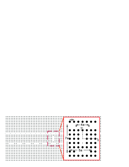
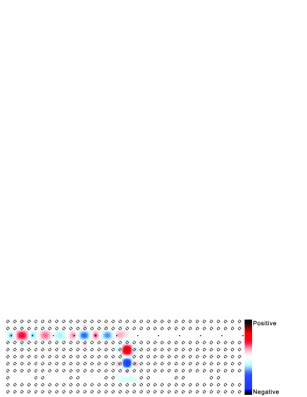
Figure 4: An experimental protocol based on a photonic crystal made up of silicon rods of radius $0.2a$. (a) The structure of the design: the upper waveguide is implemented by removing a row of original rods and substituting with a set of rods of radius $0.1a$ and spacing $d_{\mathrm{UP}}=4a$. The lower waveguide, $D=7a$ apart from the upper one, is constructed by removing three rods out of every five rods, i.e. lattice spacing $d_{\mathrm{DOWN}}=5a$. The central cavity is created by reducing the radius of three vertically-placed rods between the two waveguides to $0.05a$. (b) Plotting the steady electric field vector for an incident wave of frequency $\omega_{0}=0.3628\times 2\pi c/a$ with TM-polarization.

In conclusion, we have shown the existence of a photonic bound state in a qubit-controlled coupled resonator array and predicted photonic Feshbach resonance emerges from a pair of these coupled resonator arrays coupled in an H-shape fashion. An FDTD simulation of the system implemented on a photonic crystal has verified the validity of the proposal. The resonance phenomenon arises from the dual-channel coupling between an unbound state in one array and a bound state in the other, the occurring moment of which is indicated by a total reflection of an incident photon in the array. Our analysis for the resonant scattering process was carried out for the single photon case and did not rely on the photonic statistics. Our prediction here is thus applicable to fermionic models, such as the electron transportation along a H-shape array of quantum dots. For the case where multiple photons are assumed to exist in the arrays, Bethe-ansatz must be used for the analysis and we shall defer its discussion in a future work.

- (1) Feshbach, H. Unified theory of nuclear reactions. Ann. Phys. (N.Y.) 5, 357-390 (1958).
- (2) Pethick, C. J. & Smith, H. Bose-Einstein Condensation in Dilute Gases (Cambridge University Press, 2002).
- (3) Zhou, L., Gong, Z. R., Liu, Y.-X., Sun, C. P. & Nori, F. Controllable scattering of a single photon inside a one-dimensional resonator waveguide. Phys. Rev. Lett. 101, 100501 (2008).
- (4) Schulz, G. J. Resonances in electron impact on atoms. Rev. Mod. Phys. 45, 378-422 (1973).
- (5) ibid. Resonances in electron impact on diatomic molecules. Rev. Mod. Phys. 45, 423-486 (1973).
- (6) Courteille, P., Freeland, R. S., Heinzen, D. J., van Abeelen, F. A. & Verhaar, B. J. Observation of a feshbach resonance in cold atom scattering. Phys. Rev. Lett. 81, 69-72 (1998).
- (7) Roberts, J. L., Claussen, N. R., Burke, J. P. Jr., Greene, C., Cornell, E. A. & Wieman C. E. Resonant magnetic field control of elastic scattering in cold 85Rb. Phys. Rev. Lett. 81, 5109-5112 (1998).
- (8) Vuletic, V., Kerman, A. J., Chin, C. & Chu, S. Observation of low-field feshbach resonances in collisions of cesium atoms. Phys. Rev. Lett. 82, 1406-1409 (1999).
- (9) Inouye, S., Andrews, M. R., Stenger, J., Miesner, H. J., Stamper-Kurn, D. M. & Ketterle, W. Observation of Feshbach resonances in a Bose-Einstein condensate. Nature 392, 151-154 (1998).
- (10) Timmermans, E., Tommasini, P., Hussein, M. & Kerman, A. Feshbach resonances in atomic Bose-Einstein condensates. Phys. Rep. 315, 199-230 (1999).
- (11) Jin, D. S. & Regal, C. A. Proceedings of the International school of physics Enrico Fermi, course CLXIV (IOS Press, Amsterdam, 2008).
- (12) Loftus, T., Regal, C. A., Ticknor, C., Bohn, J. L. & Jin, D. S. Resonant control of elastic collisions in an optically trapped fermi gas of atoms. Phys. Rev. Lett. 88, 173201 (2002).
- (13) Zirbel, J. J., Ni, K.-K., Ospelkaus, S., D’Incao, J. P., Wieman, C. E., Ye, J. & Jin, D. S. Collisional stability of fermionic feshbach molecules. Phys. Rev. Lett. 100, 143201 (2008).
- (14) von Neumann, J. & Wigner, E. Üer merkwürdige diskrete Eigenwerte. Z. Phys. 30, 465-467 (1929).
- (15) Friedrich, H. & Wintgen, D. Physical realization of bound states in the continuum. Phys. Rev. A 31, 3964-3966 (1985).
- (16) Lee, T. D. Some special examples in renormalizable field theory. Phys. Rev. 95, 1329-1334 (1954).
- (17) Fano, U. Effects of configuration interaction on intensities and phase shifts. Phys. Rev. 124, 1866-1878 (1961).
- (18) Anderson, P. W. Localized magnetic states in metals. Phys. Rev. 124, 41-53 (1961).
- (19) Nakamura, H., Hatano, N., Garmon, S. & Petrosky, T. Quasibound states in the continuum in a two channel quantum wire with an adatom. Phys. Rev. Lett. 99, 210404 (2007).
- (20) Gong, Z. R., Ian, H., Zhou, L. & Sun, C. P. Controlling quasibound states in 1D continuum through electromagnetic induced transparency mechanism. arXiv:0805.3042 (2008).
- (21) Dong, H., Gong, Z. R., Ian, H., Zhou, L. & Sun, C. P. Intrinsic cavity QED and emergent quasi-normal modes for single photon. arXiv:0805.3085 (2008).
- (22) Shen, J. T. & Fan, S. Coherent single photon transport in a one-dimensional waveguide coupled with superconducting quantum bits. Phys. Rev. Lett. 95, 213001 (2005).
- (23) ibid. Strongly correlated two-photon transport in a one-dimensional waveguide coupled to a two-level system. Phys. Rev. Lett. 98, 153003 (2007).
- (24) ibid. Coherent photon transport from spontaneous emission in one-dimensional waveguides. Opt. Lett. 30, 2001-2003 (2005).
- (25) Chang, D. E., Sørensen, A. S., Demler, E. A. & Lukin, M. D. A single-photon transistor using nanoscale surface plasmons. Nature Phys. 3, 807-812 (2007).
- (26) Wallraff, A., Schuster, D. I., Blais, A., Frunzio, L., Huang, R.-S., Majer, J., Kumar, S., Girvin, S. M. & Schoelkopf, R. J. Strong coupling of a single photon to a superconducting qubit using circuit quantum electrodynamics. Nature 431, 162-167 (2004).
- (27) Fan, S., Sharp asymmetric line shapes in side-coupled waveguide-cavity systems. App. Phys. Lett. 80, 908-910 (2002).
- (28) Joannopoulus, J. D., Johnson S. G., Winn, J. N., & Meade, R. D., Photonic Crystal: Molding the flow of light (Princeton University Press, 2007).
- (29) Yariv, A., Xu, Y., Lee, R. K. & Scherer, A., Coupled-resonator optical waveguide: a proposal and analysis. Opt. Lett. 24, 711-713 (1999).
- (30) Taflove, A., & Hagness, S. C., Computational Electrodynamics: The Finite-Difference Time-Domain Method (Artech: Norwood, MA, 2000).
- (31) Farjadpour, A., Roundy, D., Rodriguez, A., Ibanescu, M., Bermel, P., Joannopoulos, J. D., Johnson, S. G., & Burr, G. Improving accuracy by subpixel smoothing in FDTD. Optics Letters 31, 2972–2974 (2006). http://ab-initio.mit.edu/wiki/index.php/Meep.