Preface

G. Bregar and N.S. Mankoč Borštnik Universidad de Zacatecas
Ap.P. 636, Suc. 3 Cruzes, C. P. 98064, Zacatecas, Zac., México
E-mail: valeri@planck.reduaz.mx
URL: http://planck.reduaz.mx/~valeri/ Universidad de Zacatecas
Ap.P. 636, Suc. 3 Cruzes, C. P. 98064, Zacatecas, Zac., México
E-mail: valeri@planck.reduaz.mx
URL: http://planck.reduaz.mx/~valeri/¹Moscow Engineering Physics Institute (National Nuclear Research University), 115409 Moscow, Russia
² Centre for Cosmoparticle Physics ”Cosmion” 125047 Moscow, Russia
³ APC laboratory 10, rue Alice Domon et Léonie Duquet
75205 Paris Cedex 13, France¹ Department of Physics, FMF, University of Ljubljana
Jadranska 19, 1000 Ljubljana, Slovenia
² Department of Physics, Niels Bohr Institute
Blegdamsvej 17,Copenhagen, DK-210014U
155 E 34 Street
New York, NY 10016 ¹Department of Physics, FMF, University of Ljubljana
Jadranska 19, 1000 Ljubljana, Slovenia
²Department of Physics, University of California, Berkeley, CA 94720, USA
³Moscow Engineering Physics Institute (National Nuclear Research University), 115409 Moscow, Russia;
Centre for Cosmoparticle Physics ”Cosmion” 125047 Moscow, Russia;
APC laboratory 10, rue Alice Domon et Léonie Duquet
75205 Paris Cedex 13, France
⁴Moscow Engineering Physics Institute (National Nuclear Research University)
115409 Moscow, RussiaSCAT, Oslo, Norway¹Moscow Engineering Physics Institute (National Nuclear Research University), 115409 Moscow, Russia
² Centre for Cosmoparticle Physics ”Cosmion” 125047 Moscow, Russia
³ APC laboratory 10, rue Alice Domon et Léonie Duquet
75205 Paris Cedex 13, France

The series of workshops on ”What Comes Beyond the Standard Model?” started in 1998 with the idea of organizing a real workshop, in which participants would spend most of the time in discussions, confronting different approaches and ideas. The picturesque town of Bled by the lake of the same name, surrounded by beautiful mountains and offering pleasant walks, was chosen to stimulate the discussions.

The idea was successful and has developed into an annual workshop, which is taking place every year since 1998. Very open-minded and fruitful discussions have become the trade-mark of our workshop, producing several published works. It takes place in the house of Plemelj, which belongs to the Society of Mathematicians, Physicists and Astronomers of Slovenia.

In this eleventh workshop, which took place from 15th to 25th of July 2008, we were discussing several topics, most of them presented in this Proceedings mainly as talks. The main topic was this time the dark matter candidates. Is the approach unifying spins and charges, proposed by Norma, which is offering the mechanism for generating families and is accordingly predicting the fourth family to be possibly seen at LHC and the stable fifth family as the candidate to form the dark matter cluster, the right way beyond the standard model? Are the clusters of the fifth family members alone what constitute the dark matter? Can the fifth family baryons explain the observed properties of the dark matter with the direct measurements included? What if such a scenario is not confirmed by the direct measurements?

Talks and discussions in our workshop are not at all talks in the usual way. Each talk or discussions lasted several hours, divided in two hours blocks, with a lot of questions, explanations, trials to agree or disagree from the audience or a speaker side. Most of talks are ”unusual” in the sense that they are trying to find out new ways of understanding and describing the observed phenomena.

New this year was the teleconference taking place during the Workshop on the theme of dark matter. It was organized by the Virtual Institute for Astrophysics (wwww.cosmovia.org) of Maxim Khlopov with able support by Didier Rouable. We managed to have ample discussions and we thank in particular Jeffrey Fillipini of Berkeley University for discussions on the CDMS experiment.

What science has learned up to now are several effective theories which, after making several starting assumptions, lead to theories (proven or not to be consistent in a way that they do not run into obvious contradictions), and which some of them are within the accuracy of calculations and experimental data, in agreement with the observations, the others might agree with the experimental data in future, and might answer at least some of the open questions, left open by the scientific community accepted effective theories. We never can say that there is no other theory which generalizes the accepted ”effective theories”, and that the assumptions made to come to an effective theory in (1+3)-dimensions are meaningful also if we allow larger number of dimensions. It is a hope that the law of Nature is simple and ”elegant”, whatever the ”elegance” might mean (besides simplicity also as few assumptions as possible), while the observed states are usually not, suggesting that the ”effective theories, laws, models” are usually very complex.

We have tried accordingly also in this workshop to answer some of the open questions which the two standard models (the electroweak and the cosmological) leave unanswered, like:

• Why has Nature made a choice of four (noticeable) dimensions while all the others, if existing, are hidden? And what are the properties of space-time in the hidden dimensions?

• How could ”Nature make the decision” about breaking of symmetries down to the noticeable ones, coming from some higher dimension d?

• Why is the metric of space-time Minkowskian and how is the choice of metric connected with the evolution of our universe(s)?

• Why do massless fields exist at all? Where does the weak scale come from?

• Why do only left-handed fermions carry the weak charge? Why does the weak charge break parity?

• Where do families come from?

• What is the origin of Higgs fields? Where does the Higgs mass come from?

• Can all known elementary particles be understood as different states of only one particle, with a unique internal space of spins and charges?

• How can all gauge fields (including gravity) be unified and quantized?

• What is our universe made out of (besides the baryonic matter)?

• What is the role of symmetries in Nature?

We have discussed these and other questions for ten days. The reader can see our progress in some of these questions in this proceedings. Some of the ideas are treated in a very preliminary way. Some ideas still wait to be discussed (maybe in the next workshop) and understood better before appearing in the next proceedings of the Bled workshops.

The organizers are grateful to all the participants for the lively discussions and the good working atmosphere. This year Workshop mostly took place at the neighboring Bled School of Management (www.iedc.si). We thank it’s director, Mr. Metod Dragonja, for kindly offering us the use of their facilities. We also thank their staff, particularly chief librarian Ms. Tanja Ovin, for providing us with excellent support.

Norma Mankoč Borštnik, Holger Bech Nielsen,
Dragan Lukman Ljubljana, December 2008

Does the Dark Matter Consist of Baryons of New Heavy Stable Family Predicted by the Approach Unifying Spins and Charges? 

G. Bregar and N.S. Mankoč Borštnik Universidad de Zacatecas
Ap.P. 636, Suc. 3 Cruzes, C. P. 98064, Zacatecas, Zac., México
E-mail: valeri@planck.reduaz.mx
URL: http://planck.reduaz.mx/~valeri/ Universidad de Zacatecas
Ap.P. 636, Suc. 3 Cruzes, C. P. 98064, Zacatecas, Zac., México
E-mail: valeri@planck.reduaz.mx
URL: http://planck.reduaz.mx/~valeri/¹Moscow Engineering Physics Institute (National Nuclear Research University), 115409 Moscow, Russia
² Centre for Cosmoparticle Physics ”Cosmion” 125047 Moscow, Russia
³ APC laboratory 10, rue Alice Domon et Léonie Duquet
75205 Paris Cedex 13, France¹ Department of Physics, FMF, University of Ljubljana
Jadranska 19, 1000 Ljubljana, Slovenia
² Department of Physics, Niels Bohr Institute
Blegdamsvej 17,Copenhagen, DK-210014U
155 E 34 Street
New York, NY 10016 ¹Department of Physics, FMF, University of Ljubljana
Jadranska 19, 1000 Ljubljana, Slovenia
²Department of Physics, University of California, Berkeley, CA 94720, USA
³Moscow Engineering Physics Institute (National Nuclear Research University), 115409 Moscow, Russia;
Centre for Cosmoparticle Physics ”Cosmion” 125047 Moscow, Russia;
APC laboratory 10, rue Alice Domon et Léonie Duquet
75205 Paris Cedex 13, France
⁴Moscow Engineering Physics Institute (National Nuclear Research University)
115409 Moscow, RussiaSCAT, Oslo, Norway¹Moscow Engineering Physics Institute (National Nuclear Research University), 115409 Moscow, Russia
² Centre for Cosmoparticle Physics ”Cosmion” 125047 Moscow, Russia
³ APC laboratory 10, rue Alice Domon et Léonie Duquet
75205 Paris Cedex 13, France

Abstract

We investigate the possibility that clusters of the heavy family of quarks and leptons with zero Yukawa couplings to the lower families constitute the dark matter. Such a family is predicted by the approach unifying spins and charges. We make a rough estimation of properties of clusters of this new family members and study limitations on the family properties due to the cosmological and the direct experimental evidences.

Abstract

We discuss transormation laws of electric and magnetic fields under Lorentz transformations, deduced from the Classical Field Theory. It is found that we can connect the resulting expression for a bivector formed with those fields, with the expression deduced from the Wigner transformation rules for spin-1 functions of massive particles. This mass parameter should be interpreted because the constancy of speed of light forbids the existence of the photon mass.

Abstract

Recently, some problems have been found in the definition of the partial derivative in the case of the presence of both explicit and implicit functional dependencies in the classical analysis. In this talk we investigate the influence of this observation on the quantum mechanics and classical/quantum field theory. Surprisingly, some commutators of the coordinate-dependent operators are not equal to zero. Therefore, we try to provide mathematical foundations to the modern non-commutative theories. We also indicate possible applications in the Dirac-like theories.

Abstract

Particle physics candidates for cosmological dark matter are usually considered as neutral and weakly interacting. However stable charged leptons and quarks can also exist and, hidden in elusive atoms, play the role of dark matter. Stable particles with charge -2 bind with primordial helium in O-helium ”atoms” (OHe), representing a specific Warmer than Cold nuclear-interacting form of dark matter. O-helium can influence primordial nucleosynthesis, giving rise, in particular, to primordial heavy elements. Its excitation in collisions in galactic bulge can lead to enhancement of positron annihilation line, observed by Integral. Slowed down in the terrestrial matter by elastic collisions, OHe is elusive for direct methods of underground Dark matter detection like those used in CDMS experiment, but its rare inelastic reactions with nuclei can lead to annual variations of energy release in the interval of energy 2-6 keV in DAMA/NaI and DAMA/Libra experiments, being consistent with the number of events registered in these experiments.

Abstract

One step towards realistic Kaluza-Klein-like theories is presented for a toy model of a spinor in $d=(1+5)$ compactified on an infinite disc with the zweibein which makes a disc curved on $S^{2}$ and with the spin connection field which allows on such a sphere only one massless spinor state of a particular charge, which couples the spinor chirally to the corresponding Kaluza-Klein gauge field. In refs. snmb1:hnkk06 ; snmb1:hn07 we achieved masslessness of spinors with the appropriate choice of a boundary on a finite disc, in this paper the masslessness is achieved with the choice of a spin connection field on a curved infinite disc.

Abstract

There are some well-known properties of our universe whose reasons are clear but strangely not well-known. Physicists seem to believe that they hold because God wants them. Actually it is usually because geometry wants them. We summarize these here; detailed discussion and proofs were given long ago (rm1nmb ; rm1nm2 ; rm1nm3 ; rm1nm4 ; rm1ia ; rm1gf ; rm1ml ; rm1pt ; rm1qm ; rm1cnfr ; rm1bna ; rm1bnb ; rm1bnc ; rm1op ; rm1cg ; rm1imp ; rm1rn ).

Abstract

The possibility that the two experiments: DAMA/NaI-LIBRA mk2disc:rita0708 and CDMS mk2disc:cdms measure the fifth family baryons predicted by the approach unifying spin and charges, proposed by N.S. Mankoč Borštnik, is discussed from the point of view of the measurements of the DAMA/NaI-LIBRA mk2disc:rita0708 and CDMS mk2disc:cdms experiments. While the DAMA/NaI-LIBRA experiment very clearly sees not only the signal but also the annual modulation of the signal, CDMS sees no signal. N. Mankoč Borštnik and G. Bregar, by estimating what is happening when the fifth family neutron hits the first family nucleon, predict that CDMS will in the near future see the fifth family baryons, if the fifth family baryons are what DAMA/NaI-LIBRA measures. M.Khlopov, A.Mayorov and E.Soldatov are proposing alternative scenario, which is applicable for the fifth family clusters and formulates the conditions, under which the results of both experiments can be explained. In these discussions J. Filippini from CDMS collaboration helped a lot to clarify what is happening in the measuring procedure of both experiments, if they do measure a heavy family cluster with small enough scattering cross section on ordinary nuclei.

Abstract

Discussion concerns the evaluation of the colour, the weak and the ”nuclear” interactions among the fifth family quarks, among the fifth family baryons and among the fifth family and ordinary baryons.

Abstract

Virtual Instutute of Astroparticle Physics (VIA) has evolved in a unique multi-functional complex, aimed to combine various forms of collaborative scientific work with programs of education on distance. The activity on VIA website includes regular video conferences with systematic basic courses and lectures on various issues of astroparticle physics, library of their records and presentations, a multilingual forum. VIA virtual rooms are open for meetings of scientific groups and for individual work of supervisors with their students. The format of a VIA video conference was used in the program of Bled Workshop to discuss the puzzles of dark matter searches.

0.1 Introduction

Although the origin of the dark matter is unknown, its gravitational interaction with the known matter and other cosmological observations require that a candidate for the dark matter constituent has the following properties:

• i. The scattering amplitude of a cluster of constituents with the ordinary matter and among the dark matter clusters themselves must be small enough to be in agreement with the observations (so that no effect of such scattering has been observed, except possibly in the DAMA experiments rita0708 ).
  

• ii. Its density distribution (obviously different from the ordinary matter density distribution) within a galaxy is approximately spherically symmetric and decreases approximately with the second power of the radius of the galaxy. It is extended also far out of the galaxy, manifesting the gravitational lensing by galaxy clusters.
  

• iii. The dark matter constituents must be stable in comparison with the age of our universe, having obviously for many orders of magnitude different time scale for forming (if at all) matter than the ordinary matter.
  

• iv. The dark matter constituents and accordingly also the clusters had to have a chance to be formed during the evolution of our universe so that they contribute today the main part of the matter in the universe. The ratio of the dark matter density and the baryon matter density is evaluated to be 5-7.
  

Candidates for the dark matter constituents may give the explanation for the non agreement between the two direct measurements of the dark matter constituents rita0708 ; cdms , provided that they measure a particular candidate.

There are several candidates for the massive dark matter constituents in the literature, known as WIMPs (weakly interacting massive particles), the references can be found in dodelson ; rita0708 .

In this talk the possibility that the dark matter constituents are clusters of a stable (from the point of view of the age of the universe) family of quarks and leptons is discussed. Such a family is predicted by the approach unifying spin and charges pn06 ; n92 ; n93 ; n07bled ; gmdn07 , proposed by N.S.M.B..

There are several attempts in the literature to explain the origin of families, all in one or another way just postulating that there are at least three families, as does the standard model of the electroweak and colour interactions. Proposing the (right) mechanism for generating families is therefore one of the most promising guides to understanding physics beyond the standard model. The approach unifying spins and charges is offering a mechanism for the appearance of families. It introduces the second kind pn06 ; n92 ; n93 ; n07bled ; hn02hn03 of the Clifford algebra objects, which generates families by defining the equivalent representations with respect to the Dirac spinor representation . The approach predicts more than the observed three families. It predicts two times four families with masses several orders of magnitude bellow the unification scale of the three observed charges. Since due to the approach (if a particular way of breaking the starting symmetry is assumed) the fifth family decouples in the Yukawa couplings from the lower four families gmdn07 , the quarks and the leptons of the fifth family are stable as required by the condition iii.. Since the masses of the fifth family lie much above the known three and the predicted fourth family masses (the fourth family might according to the first very rough estimates be even seen at LHC), the baryons made out of the fifth family are heavy, forming small enough clusters, so that their scattering amplitude among themselves and with the ordinary matter is small enough and also the number of clusters forming the dark matter is low enough to fulfil the conditions i. and iii..

We make a rough estimation of properties of clusters of the members of the fifth family ($u_{5},d_{5},\nu_{5},e_{5}$), which in the approach unifying spin and charges have all the properties of the lower four families: the same family members with the same charges $U(1),SU(2)$ and $SU(3)$, and interact correspondingly with the same gauge fields.

We use a simple (the Bohr-like) model gnBled07 to estimate the size and the binding energy of the fifth family baryons, assuming that the fifth family quarks are heavy enough to interact mainly exchanging one gluon. We estimate the behaviour of quarks and anti-quarks of the fifth family under the assumption that during the evolution of the universe quarks and anti-quarks mostly succeeded to form neutral (with respect to the colour and electromagnetic charge) clusters, which now form the dark matter. We also estimate the behaviour of our fifth family clusters if hitting the DAMA/NaI, DAMA-LIBRA rita0708 and CDMS cdms experiments.

All estimates are very approximate and need serious additional studies. Yet we believe that such rough estimations give a guide to further studies.

0.2 The approach unifying spin and charges

The approach unifying spin and charges pn06 ; n92 ; n93 ; n07bled ; gmdn07 motivates the assumption that clusters of the fifth heavy stable (with respect to the age of the universe) family members form the dark matter. The approach assumes that in $d\geq(1+13)$-dimensional space a Weyl spinor carries nothing but two kinds of spins (no charges): The Dirac spin described by $\gamma^{a}$’s defines the ordinary spinor representation, the second kind of spin hn02hn03 described by $\tilde{\gamma}^{a}$’s, anticommuting with the Dirac one, defines the families of spinors . Spinors interact with the gravitational gauge fields: vielbeins and two kinds of spin connections. A simple starting Lagrange density for a spinor and for gauge fields in $d=1+13$ manifests, after the appropriate breaks of symmetries, in $d=1+3$ all the properties of the spinors (fermions) and the gauge fields assumed by the standard model of the electroweak and colour interaction, with the Yukawa couplings included. The approach offers accordingly the explanation for the appearance of families (see ref. pn06 ; n92 ; n93 ; n07bled ; gmdn07 and the references cited in these references) and predicts two times four families with zero (that is negligible with respect to the age of the universe) Yukawa couplings among the two groups of families at low energy region. In the very rough estimations gmdn07 the fourth family masses are predicted to be at rather low energies (at around 250 GeV or higher). so that it might be seen at LHC. The lightest of the next four families is the candidate to form the dark matter . The energy range, in which the masses of the fifth family quarks might appear, is far above $300$ GeV (say higher than $10^{4}\;{\rm GeV}$ and much lower than the scale of the break of $SO(4)\times U(1)$ to $SU(2)\times U(1)$, which might occur at $10^{13}$ GeV hnproc02 ).

0.3 Properties of clusters of a heavy family

Let us assume that there is a heavy family of quarks and leptons as predicted by the approach unifying spins and charges: i. It has masses several orders of magnitude greater than the known three families. ii. The matrix elements with the lower families in the mixing matrix (the Yukawa couplings) are equal to zero. iii. All the charges ($SU(3),SU(2),U(1)$ and correspondingly after the break of the electroweak symmetry $SU(3),U(1)$) are those of the known families and so are accordingly also the couplings to the gauge fields. Families distinguish among themselves in the family index (in the quantum number, which in the approach is determined by the operators $\tilde{S}^{ab}=\frac{i}{4}(\tilde{\gamma}^{a}\tilde{\gamma}^{b}-\tilde{\gamma}^{b}\tilde{\gamma}^{a})$), and (due to the Yukawa couplings) in their masses.

For a heavy enough family the properties of baryons (neutrons $n_{5}$ $(u_{5}d_{5}d_{5})$, protons $(u_{5}u_{5}d_{5})$, $\Delta_{5}^{-}$ $(u_{5}u_{5}d_{5})$, $\Delta_{5}^{++}$ $(u_{5}u_{5}u_{5})$, e.t.c), made out of the quarks $u_{5}$ and $d_{5}$ can be estimated by using the non relativistic Bohr-like model with the $\frac{1}{r}$ (radial) dependence of the potential between a pair of quarks $V=-\frac{3\alpha_{c}}{r}$, where $\alpha_{c}$ is in this case the colour (3 for three possible colour charges) coupling constant. Equivalently goes for anti-quarks. This is a meaningful approximation as long as one gluon exchange contribution to the interaction among quarks is a dominant contribution (which means: as long as excitations of a cluster are not influenced by the linearly rising part of the potential).

Which one of $p_{5}$, $n_{5}$ or maybe $\Delta^{-}$ or $\Delta^{++}$ is a stable fifth family baryon, depends on the ratio of the bare masses $m_{u_{5}}$ and $m_{d_{5}}$, as well as on the weak and electromagnetic interactions among quarks. If $m_{d_{5}}$ is appropriately lighter than $m_{u_{5}}$ so that the repulsive weak and electromagnetic interactions favors the neutron $n_{5}$, then $n_{5}$ is a colour singlet electromagnetic chargeless stable cluster of quarks with the lowest mass among the nucleons of the fifth family, with the weak charge $-1/2$.

If $m_{d_{5}}$ is heavier (enough, due to stronger electromagnetic repulsion among the two $u_{5}$ than among the two $d_{5}$) than $m_{u_{5}}$, the proton $p_{5}$, which is a colour singlet stable nucleon, needs the electron $e_{5}$ or $e_{1}$ to form an electromagnetic chargeless cluster. (Such an electromagnetic and colour chargeless cluster has also the expectation value of the weak charge equal to zero.)

An atom made out of only fifth family members might be lighter or not than $n_{5}$, depending on the masses of the fifth family members. We shall for simplicity assume in this first rough estimations that $n_{5}$ is a stable baryon and equivalently also $\bar{n}_{5}$, leaving all the other possibilities for further studies gmn08 .

In the Bohr-like model, when neglecting more than one gluon exchange contribution (the simple bag model evaluation does not contradict such a simple model , while the electromagnetic and weak interaction contribution is more than $10^{-3}$ times smaller) the binding energy and the average radius are equal to

$$E_{c_{5}}=-\frac{3}{2}\,m_{q_{5}}c^{2}(3\alpha_{c})^{2},\quad r_{c_{5}}=\frac{\hbar c}{3\alpha_{c}m_{q_{5}}c^{2}}$$ (1)

The mass of the cluster is approximately $m_{c_{5}}c^{2}=3m_{q_{5}}c^{2}(1-\frac{1}{2}(3\alpha_{c})^{2})$ (if $n_{5}$ is the stable baryon, since we take that the space part of the wave function is symmetric and also the spin and the weak charge part, each of a mixed symmetry, couple to symmetric wave function, we neglect the weak and the electromagnetic interaction). Assuming that the coupling constant of the colour charge $\alpha_{c}$ runs with the kinetic energy $E$ of quarks as in ref. greiner with the number of flavours $N_{F}=8$ ($\,\alpha_{c}(E^{2})=\frac{\alpha_{c}(M^{2})}{1+\frac{\alpha_{c}(M^{2})}{4\pi}(11-\frac{2N_{F}}{3})\textrm{ln}(\frac{E^{2}}{M^{2}})}$, with $\alpha_{c}((91\;\textrm{GeV})^{2})=0.1176(20)$ ) we estimated the properties of a baryon as presented on Table 1.

$\frac{m_{q_{5}}c^{2}}{{\rm TeV}}$	$\alpha_{c}$	$\frac{E_{c_{5}}}{{\rm TeV}}$	$\frac{r_{c5}}{10^{-7}{\rm fm}}$	$\frac{\pi r_{c5}^{2}}{(10^{-7}{\rm fm})^{2}}$
$10^{2}$	0.09	5.4	150	$6.8\cdot 10^{4}$
$10^{4}$	0.07	$3\cdot 10^{2}$	1.9	12
$10^{6}$	0.05	$2\cdot 10^{4}$	0.024	$1.9\cdot 10^{-3}$

Table 1: Properties of a cluster of the fifth family quarks within the Bohr-like model. $m_{q_{5}}$ in TeV/c² is the assumed fifth family quark mass, $\alpha_{c}$ is the coupling constant of the colour interaction at $E\approx(-E_{c_{5}}/3)$ (Eq.(1)), which is the kinetic energy of the quarks in the cluster, $r_{c5}$ is the corresponding Bohr-like radius, $\sigma_{c5}=\pi r_{c5}^{2}$ is the corresponding scattering cross section for a chosen quark mass.

The binding energy is approximately of two orders of magnitude smaller than the mass of the cluster. The $n_{5}$ ($u_{q_{5}}d_{q_{5}}d_{q_{5}}$) cluster is lighter than cluster $p_{5}$ ($u_{q_{5}}d_{q_{5}}d_{q_{5}}$) if $(m_{u_{5}}-m_{d_{5}})$ is smaller then $(0.6,60,600)$ GeV for the three values of the $m_{q_{5}}$ on Table 1, respectively. We clearly see that the ”nucleon-nucleon force” among the fifth family baryons leads to for many orders of magnitude smaller scattering than among the first family baryons.

The scattering cross section between two clusters of the fifth family quarks is determined by the weak interaction as soon as the mass exceeds several GeV.

If a cluster of the heavy (fifth family) quarks and leptons and of the ordinary (the lightest) family is made, then, since ordinary family dictates the radius and the excitation energies of a cluster, its properties are not far from the properties of the ordinary hadrons and atoms, except that such a cluster has the mass dictated by the heavy family members.

0.4 Dynamics of a heavy family clusters in our galaxy

The density of the dark matter $\rho_{dm}$ in the Milky way can be evaluated from the measured rotation velocity of stars and gas in our galaxy, which is approximately constant (independent of the distance from the center of our galaxy). For our Sun this velocity is $v_{S}\approx(170-270)$ km/s. Locally $\rho_{dm}$ is known within a factor of 10 to be $\rho_{0}\approx 0.3\,{\rm GeV}/(c^{2}\,{\rm cm}^{3})$, we put $\rho_{dm}=\rho_{0}\,\varepsilon_{\rho},$ with $\frac{1}{3}<\varepsilon_{\rho}<3$. The local velocity of the dark matter cluster $\mathchoice{\mbox{\boldmath$\displaystyle v$}}{\mbox{\boldmath$\textstyle v$}}{\mbox{\boldmath$\scriptstyle v$}}{\mbox{\boldmath$\scriptscriptstyle v$}}_{dm}$ is model dependant. In a simple model that all the clusters at any radius $r$ from the center of our galaxy rotate in circles way around the center, so that the paths are spherically symmetrically distributed, the velocity of a cluster at the position of the Earth is equal to $v_{S}$, the velocity of our Sun in the absolute value, but has all possible orientations perpendicular to the radius $r$ with equal probability. In the model that all the clusters oscillate through the center of the galaxy, the velocities of the dark matter clusters at the Earth position have values from zero to the escape velocity, each one weighted so that all the contributions give $\rho_{dm}$. Also the model that clusters make all possible paths from the oscillatory one to the circle, weighted so that they reproduce the $\rho_{dm}$, seems acceptable. Many other possibilities are presented in the references of rita0708 .

The velocity of the Earth around the center of the galaxy is equal to: $\mathchoice{\mbox{\boldmath$\displaystyle v$}}{\mbox{\boldmath$\textstyle v$}}{\mbox{\boldmath$\scriptstyle v$}}{\mbox{\boldmath$\scriptscriptstyle v$}}_{E}=\mathchoice{\mbox{\boldmath$\displaystyle v$}}{\mbox{\boldmath$\textstyle v$}}{\mbox{\boldmath$\scriptstyle v$}}{\mbox{\boldmath$\scriptscriptstyle v$}}_{S}+\mathchoice{\mbox{\boldmath$\displaystyle v$}}{\mbox{\boldmath$\textstyle v$}}{\mbox{\boldmath$\scriptstyle v$}}{\mbox{\boldmath$\scriptscriptstyle v$}}_{ES}$, with $v_{ES}=30$ km/s. Then the velocity with which the dark matter hits the Earth is equal to: $\mathchoice{\mbox{\boldmath$\displaystyle v$}}{\mbox{\boldmath$\textstyle v$}}{\mbox{\boldmath$\scriptstyle v$}}{\mbox{\boldmath$\scriptscriptstyle v$}}_{dmE\,i}=\mathchoice{\mbox{\boldmath$\displaystyle v$}}{\mbox{\boldmath$\textstyle v$}}{\mbox{\boldmath$\scriptstyle v$}}{\mbox{\boldmath$\scriptscriptstyle v$}}_{dm\,i}-\mathchoice{\mbox{\boldmath$\displaystyle v$}}{\mbox{\boldmath$\textstyle v$}}{\mbox{\boldmath$\scriptstyle v$}}{\mbox{\boldmath$\scriptscriptstyle v$}}_{E}$, where the index $i$ stays for the $i$-th velocity class.

Let us evaluate the cross section for a heavy dark matter cluster to elastically scatter on an ordinary nucleus with $A$ nucleons in the Born approximation: $\sigma_{c_{5}A}=\frac{m_{A}^{2}}{\pi\hbar^{2}}<|M_{c_{5}A}|>^{2}$. For our heavy dark matter cluster with a small cross section from Table 1 is $m_{A}$ approximately the mass of the ordinary nucleus. If the mass of the cluster is around $1$ TeV or more and its velocity $\approx v_{S}$, is $\lambda=\frac{h}{p_{A}}$ for a nucleus large enough to make scattering totally coherent. The cross section is almost independent of the recoil velocity of the nucleus. (We are studying this problem intensively.) For masses of quarks $m_{q_{5}}<10^{4}$ TeV (when the ”nucleon-nucleon force” dominates) is the cross section proportional to $(3A)^{2}$ (due to the square of the matrix element) times $(A)^{2}$ (due to the mass of the nuclei $m_{A}\approx 3A\,m_{q_{1}}$, with $m_{q_{1}}$ which is the first family dressed quark mass), so that $\sigma(\mathchoice{\mbox{\boldmath$\displaystyle v$}}{\mbox{\boldmath$\textstyle v$}}{\mbox{\boldmath$\scriptstyle v$}}{\mbox{\boldmath$\scriptscriptstyle v$}}_{dmEi},A)=\sigma(A)\propto A^{4}$. Estimated with the Bohr-like model (Table 1) $\sigma(\mathchoice{\mbox{\boldmath$\displaystyle v$}}{\mbox{\boldmath$\textstyle v$}}{\mbox{\boldmath$\scriptstyle v$}}{\mbox{\boldmath$\scriptscriptstyle v$}}_{dmEi},A)=\sigma_{0}\,\varepsilon_{\sigma}\,A^{4},$ with $\frac{1}{30}<\varepsilon_{\sigma}<30$ and $\sigma_{0}=9\,\pi r_{c_{5}}^{2}$. For masses of the fifth family quarks $m_{q_{5}}>10^{4}$ TeV, the weak interaction starts to dominate. In this case the scattering cross section is $\sigma(\mathchoice{\mbox{\boldmath$\displaystyle v$}}{\mbox{\boldmath$\textstyle v$}}{\mbox{\boldmath$\scriptstyle v$}}{\mbox{\boldmath$\scriptscriptstyle v$}}_{dmEi},A)=(\frac{m_{n_{1}}\,A\,(A-Z)G_{F}}{\sqrt{2\pi}})^{2}\varepsilon_{\sigma_{weak}}$ ($\approx(10^{-6}\,{\rm fm}\,\,A^{2}\,\frac{A-Z}{A})^{2}\,\varepsilon_{\sigma_{weak}}$) $=\sigma_{0}\,A^{4}\,\varepsilon_{\sigma_{weak}}$, with $\sigma_{0}=(\frac{m_{n_{1}}\,(A-Z)G_{F}}{A\,\sqrt{2\pi}})^{2}$ and $\varepsilon_{\sigma_{weak}}\approx 1$ (the weak force is pretty accurately evaluated, however, taking into account the threshold of a measuring apparatus may change the results obtained with the averaging assumptions presented above).

We find accordingly for the flux per unit time and unit surface of our (any heavy with the small enough cross section) dark matter clusters hitting the Earth $\Phi_{dm}=\sum_{i}\,\frac{\rho_{dmi}}{m_{c_{5}}}\,|\mathchoice{\mbox{\boldmath$\displaystyle v$}}{\mbox{\boldmath$\textstyle v$}}{\mbox{\boldmath$\scriptstyle v$}}{\mbox{\boldmath$\scriptscriptstyle v$}}_{dmi}-\mathchoice{\mbox{\boldmath$\displaystyle v$}}{\mbox{\boldmath$\textstyle v$}}{\mbox{\boldmath$\scriptstyle v$}}{\mbox{\boldmath$\scriptscriptstyle v$}}_{E}|$ to be approximately (as long as $\frac{v_{ES}}{|\mathchoice{\mbox{\boldmath$\displaystyle v$}}{\mbox{\boldmath$\textstyle v$}}{\mbox{\boldmath$\scriptstyle v$}}{\mbox{\boldmath$\scriptscriptstyle v$}}_{dmi}-\mathchoice{\mbox{\boldmath$\displaystyle v$}}{\mbox{\boldmath$\textstyle v$}}{\mbox{\boldmath$\scriptstyle v$}}{\mbox{\boldmath$\scriptscriptstyle v$}}_{S}|}$ is small) equal to:

$$\Phi_{dm}\approx\sum_{i}\,\frac{\rho_{dmi}}{m_{c_{5}}}\,\{|\mathchoice{\mbox{\boldmath$\displaystyle v$}}{\mbox{\boldmath$\textstyle v$}}{\mbox{\boldmath$\scriptstyle v$}}{\mbox{\boldmath$\scriptscriptstyle v$}}_{dmi}-\mathchoice{\mbox{\boldmath$\displaystyle v$}}{\mbox{\boldmath$\textstyle v$}}{\mbox{\boldmath$\scriptstyle v$}}{\mbox{\boldmath$\scriptscriptstyle v$}}_{S}|-\mathchoice{\mbox{\boldmath$\displaystyle v$}}{\mbox{\boldmath$\textstyle v$}}{\mbox{\boldmath$\scriptstyle v$}}{\mbox{\boldmath$\scriptscriptstyle v$}}_{ES}\cdot\frac{\mathchoice{\mbox{\boldmath$\displaystyle v$}}{\mbox{\boldmath$\textstyle v$}}{\mbox{\boldmath$\scriptstyle v$}}{\mbox{\boldmath$\scriptscriptstyle v$}}_{dmi}-\mathchoice{\mbox{\boldmath$\displaystyle v$}}{\mbox{\boldmath$\textstyle v$}}{\mbox{\boldmath$\scriptstyle v$}}{\mbox{\boldmath$\scriptscriptstyle v$}}_{S}}{|\mathchoice{\mbox{\boldmath$\displaystyle v$}}{\mbox{\boldmath$\textstyle v$}}{\mbox{\boldmath$\scriptstyle v$}}{\mbox{\boldmath$\scriptscriptstyle v$}}_{dmi}-\mathchoice{\mbox{\boldmath$\displaystyle v$}}{\mbox{\boldmath$\textstyle v$}}{\mbox{\boldmath$\scriptstyle v$}}{\mbox{\boldmath$\scriptscriptstyle v$}}_{S}|}\}.$$ (2)

We neglected further terms. The flux is very much model dependent. We shall approximately take that

$$\sum_{i}\,|\mathchoice{\mbox{\boldmath$\displaystyle v_{dmi}$}}{\mbox{\boldmath$\textstyle v_{dmi}$}}{\mbox{\boldmath$\scriptstyle v_{dmi}$}}{\mbox{\boldmath$\scriptscriptstyle v_{dmi}$}}-\mathchoice{\mbox{\boldmath$\displaystyle v_{S}$}}{\mbox{\boldmath$\textstyle v_{S}$}}{\mbox{\boldmath$\scriptstyle v_{S}$}}{\mbox{\boldmath$\scriptscriptstyle v_{S}$}}|\,\rho_{dmi}=\varepsilon_{v_{dmS}}\,\varepsilon_{\rho}\,v_{S}\,\rho_{0},$$

(with $\rho_{0}=0.3\,{\rm GeV}/(c^{2}\,{\rm cm}^{3})$) while we estimate

$$\sum_{i}\,\mathchoice{\mbox{\boldmath$\displaystyle v$}}{\mbox{\boldmath$\textstyle v$}}{\mbox{\boldmath$\scriptstyle v$}}{\mbox{\boldmath$\scriptscriptstyle v$}}_{ES}\cdot\frac{\mathchoice{\mbox{\boldmath$\displaystyle v$}}{\mbox{\boldmath$\textstyle v$}}{\mbox{\boldmath$\scriptstyle v$}}{\mbox{\boldmath$\scriptscriptstyle v$}}_{dmi}-\mathchoice{\mbox{\boldmath$\displaystyle v$}}{\mbox{\boldmath$\textstyle v$}}{\mbox{\boldmath$\scriptstyle v$}}{\mbox{\boldmath$\scriptscriptstyle v$}}_{S}}{|\mathchoice{\mbox{\boldmath$\displaystyle v$}}{\mbox{\boldmath$\textstyle v$}}{\mbox{\boldmath$\scriptstyle v$}}{\mbox{\boldmath$\scriptscriptstyle v$}}_{dmi}-\mathchoice{\mbox{\boldmath$\displaystyle v$}}{\mbox{\boldmath$\textstyle v$}}{\mbox{\boldmath$\scriptstyle v$}}{\mbox{\boldmath$\scriptscriptstyle v$}}_{S}|}=v_{ES}\varepsilon_{v_{dmES}}\cos\theta\,\sin\omega t,$$

$\theta=60^{0}$, $\frac{1}{3}<\frac{\varepsilon_{v_{dmES}}}{\varepsilon_{v_{dmS}}}<3$ and $\omega$ determined by one year rotation of our Earth around our Sun.

0.5 Direct measurements of the fifth family baryons as dark matter constituents

Assuming that the DAMA rita0708 and CDMS cdms experiments are measuring the fifth family neutrons, we are estimating properties of $q_{5}$ ($u_{5},d_{5}$). We discussed our rough estimations with Rita Bernabei privatecommRBJF and Jeffrey Filippini privatecommRBJF and both were very clear that one can hardly compare both experiments (R.B. in particular), and that the details about the way how do the dark matter constituents scatter on the nuclei and with which velocity do they scatter (in ref. rita0708 such studies were done) as well as how does a particular experiment measure events are very important, and that the results depend very significantly on the details, which might change the results for orders of magnitude. We are completely aware of how rough our estimation is, yet we see, since the number of measuring events is inversely proportional to the third power of clusters’ mass when the ”nuclear force” dominates for $m_{q_{5}}<10^{4}$ TeV, that even such rough estimations may in the case of our (any) heavy dark matter clusters say, whether both experiments do at all measure our (any) heavy family clusters, if one experiment clearly sees the dark matter signals and the other does not (yet?).

Let $N_{A}$ be the number of nuclei of type $A$ in the detectors (of either DAMA rita0708 , which has $4.0\cdot 10^{24}$ nuclei of $I$, with $A_{I}=127$ nuclei per kg and the same number of $Na$, with $A_{Na}=23$ or of CDMS cdms , which has $8.3\cdot 10^{24}$ $Ge$ nuclei, with $A_{Ge}=73$ per kg). At velocities of a dark matter cluster $v_{dmE}$ $\approx$ $200$ km/s are the $3A$ scatterers strongly bound in the nucleus, so that if hitting one quark the whole nucleus with $A$ nucleons recoils and accordingly elastically scatters on a heavy dark matter cluster. Then the number of events per second ($R_{A}$) taking place in $N_{A}$ nuclei is due to Eq. 2 and the recognition that the cross section is at these energies almost independent of the velocity (and depends accordingly only on $A$ of the nucleus), equal to

$$R_{A}=\,N_{A}\,\frac{\rho_{0}}{m_{c_{5}}}\;\sigma(A)\,v_{S}\,\varepsilon_{v_{dmS}}\,\varepsilon_{\rho}\,(1+\frac{\varepsilon_{v_{dmES}}}{\varepsilon_{v_{dmS}}}\,\frac{v_{ES}}{v_{S}}\,\cos\theta\,\sin\omega t).$$ (3)

Let $\Delta R_{A}$ mean the amplitude of the annual modulation of $R_{A}$ $\Delta R_{A}=R_{A}(\omega t=\frac{\pi}{2})-R_{A}(\omega t=0)$. Then $R_{A}(\sin\omega t=1)=N_{A}\,R_{0}\,A^{4}\,\frac{\varepsilon_{v_{dmES}}}{\varepsilon_{v_{dmS}}}\,\frac{v_{ES}}{v_{S}}\,\cos\theta$, where $R_{0}=\sigma_{0}\,\frac{\rho_{0}}{3\,m_{q_{5}}}\,v_{S}\,\varepsilon$, and $R_{0}$ is for the case that the ”nuclear force” dominates $R_{0}=\pi\,(\frac{\hbar\,c}{\alpha_{c}\,m_{q_{5}}\,c^{2}})^{2}\,\frac{\rho_{0}}{m_{q_{5}}}\,v_{S}\,\varepsilon$, with $\varepsilon=\varepsilon_{\rho}\,\varepsilon_{v_{dmES}}\varepsilon_{\sigma}$. $R_{0}$ is therefore proportional to $m_{q_{5}}^{-3}$. We estimated $\frac{1}{300}<\varepsilon<300$, which demonstrates both, the uncertainties in the knowledge about the dark matter dynamics in our galaxy and our approximate treating of the dark matter properties. When for $m_{q_{5}}\,c^{2}>10^{4}$ TeV the weak interaction determines the cross section, $R_{0}$ is in this case proportional to $m_{q_{5}}^{-1}$.

We estimate that an experiment with $N_{A}$ scatterers should measure $R_{A}\varepsilon_{cut}$, with $\varepsilon_{cut}$ determining the efficiency of a particular experiment to detect a dark matter cluster collision. $\varepsilon_{cut}$ takes into account the threshold of a detector. Although the scattering cross section is independent of the energy, the number of detected events depends on the velocity of the dark matter clusters, due to the angular distribution of the scattered nuclei and due to the energy threshold of the detector, which is not included in $\varepsilon_{v_{dmS}}$. For small enough $\frac{\varepsilon_{v_{dmES}}}{\varepsilon_{v_{dmS}}}\,\frac{v_{ES}}{v_{S}}\,\cos\theta$ we have

$$R_{A}\,\varepsilon_{cut}\approx N_{A}\,R_{0}\,A^{4}\,\varepsilon_{cut}=\Delta R_{A}\varepsilon_{cut}\,\frac{\varepsilon_{v_{dmS}}}{\varepsilon_{v_{dmES}}}\,\frac{v_{S}}{v_{ES}\,\cos\theta}.$$ (4)

If DAMA rita0708 is measuring our (any) heavy dark matter clusters scattering mostly on $I$ (we shall neglect the same number of $Na$, with $A=23$), then

$$R_{I}\,\varepsilon_{cut\,dama}\approx\Delta R_{I}\;\varepsilon_{cut\,dama}\,\frac{\varepsilon_{v_{dmS}}}{\varepsilon_{v_{dmES}}}\,\frac{v_{S}}{v_{SE}\,\cos\theta}.$$

In this rough estimation most of unknowns, except the local velocity of our Sun, the cut off procedure ($\varepsilon_{cut\,dama}$) and $\frac{\varepsilon_{v_{dmS}}}{\varepsilon_{v_{dmES}}}$, are hidden in $\Delta R_{0}$. If we assume that the Sun’s velocity is $v_{S}=100,170,220,270$ km/s, we find $\frac{v_{S}}{v_{SE}\cos\theta}=7$, $10$, $14$, $18$, respectively. The recoil energy of the nucleus $A=I$ changes correspondingly with the square of $v_{S}$. DAMA rita0708 publishes $\varepsilon_{cut\,dama}\,\Delta R_{I}=0,052$ counts per day and per kg of NaI. Correspondingly is $R_{I}\,\varepsilon_{cut\,dama}=0,052\,\frac{\varepsilon_{v_{dmS}}}{\varepsilon_{v_{dmES}}}\,\frac{v_{S}}{v_{SE}\cos\theta}$ counts per day and per kg.

CDMS should then in $121$ days with 1 kg of Ge ($A=73$) detect $R_{Ge}\,\varepsilon_{cut\,cdms}$ $\approx\frac{8.3}{4.0}\,(\frac{73}{127})^{4}\;\frac{\varepsilon_{cut\,cdms}}{\varepsilon_{cut\,dama}}\,\frac{\varepsilon_{v_{dmS}}}{\varepsilon_{v_{dmES}}}\;\frac{v_{S}}{v_{SE}\cos\theta}\;0.052\cdot 121\;$ events, which is for the above measured velocities equal to $(10,16,21,25)\,\frac{\varepsilon_{cut\,cdms}}{\varepsilon_{cut\,dama}}\;\frac{\varepsilon_{v_{dmS}}}{\varepsilon_{v_{dmES}}}$. CDMS cdms has found no event.

The approximations we made might cause that the expected numbers $(10$, $16$, $21$, $25)$ multiplied by $\frac{\varepsilon_{cut\,cdms}}{\varepsilon_{cut\,dama}}\;\frac{\varepsilon_{v_{dmS}}}{\varepsilon_{v_{dmES}}}$ are too high for a factor let us say $4$ or $10$. (But they also might be too low for the same factor!) If in the near future CDMS (or some other equivalent experiment) will measure the above predicted events, then there might be heavy family clusters which form the dark matter. In this case the DAMA experiment put the limit on our heavy family masses (Eq.(4)). In this case the DAMA experiments puts the limit on our heavy family masses (Eq.(4)). Taking into account the uncertainties in the ”nuclear force” cross section, we evaluate the lower limit for the mass $m_{q_{5}}\,c^{2}>200$ TeV. Observing that for $m_{q_{5}}\,c^{2}>10^{4}$ TeV the weak force starts to dominate, we estimate the upper limit $m_{q_{5}}\,c^{2}<10^{5}$ TeV. In the case that the weak interaction determines the $n_{5}$ cross section we find for the mass range $10\,{\rm TeV}<m_{q_{5}}\,c^{2}<10^{5}$ TeV.

0.6 Evolution of the abundance of the fifth family members in the universe

There are several questions to which we would need the answers before estimating the behaviour of our heavy family in the expanded universe, like: What is the particle—anti-particle asymmetry for the fifth family? What are the fifth family masses? How are gluons and quark—anti-quark pairs of the fifth family members (nonperturbatively) ”dressing” the quarks of the fifth family, after the quarks decouple from the rest of the cosmic plasma in the expanding universe and how do quarks form baryons? And others. We are not yet able to answer these questions. (These difficult studies are under considerations.)

We shall simply assume that there are clusters of baryons and anti-baryons of the fifth family quarks constituting the dark matter. We estimate a possible evolution of the fifth family members’ abundance when $q_{5}$ and $\bar{q}_{5}$ are in the equilibrium with the cosmic plasma (to which all the families with lower masses and all the gauge fields contribute) decoupling from the plasma at the temperature $T_{1}\approx m_{q_{5}}c^{2}/k_{b}$, with $k_{b}$ the Boltzmann constant, of the fifth family quarks and anti-quarks, assuming that the quarks and anti-quarks form (recombine into) the baryons $n_{5}$ and $\bar{n}_{5}$. (Namely, when at $T_{1}$ the fifth family quarks’ (as well as the anti-quarks’) scattering amplitude is too low to keep the quarks at equilibrium with the plasma, quarks loose the contact with the plasma. The gluon interaction, however, sooner or later either causes the annihilation of quarks and anti-quarks, or forces the quarks and anti-quarks to form baryons and anti-baryons, which are colour neutral (reheating the plasma). We are studying these possibilities in more details in gmn08 . Here we present the results of the very rough estimations, which need to be studied in more details.)

To estimate the number of the fifth family quarks and anti-quarks clustered into $n_{5}$ and $\bar{n}_{5}$ we follow the ref. dodelson , chapter 3. Let $\Omega_{5}=\frac{\rho_{c_{5}}}{\rho_{cr}}$ ($\rho_{cr}=\frac{3H_{0}^{2}}{8\pi G}$, $H_{0}$ is the present Hubble constant and $G$ is the gravitational constant) denote the ratio between the abundance of the fifth family clusters and the ordinary baryons (made out of the first family quarks), which is estimated to be $\approx 0.1$. It follows

$$\Omega_{5} = \frac{1}{\beta}\,\frac{T_{1}k_{B}}{m_{c_{5}}c^{2}}\,\sqrt{g^{*}}\,(\frac{a(T_{1})T_{1}}{a(T_{0})T_{0}})^{3}\,\sqrt{\frac{4\pi^{3}G}{45(\hbar\,c)^{3}}}\,\frac{(T_{0}\,k_{b})^{3}}{\rho_{cr}c^{4}}\frac{1}{<\sigma_{5}\,v/c>}$$ (5)

where we evaluated $\frac{T_{1}k_{B}}{m_{c_{5}}c^{2}}\,(\frac{a(T_{1})T_{1}}{a(T_{0})T_{0}})^{3}\approx 10^{-3}$. $T_{0}$ is the today’s black body radiation temperature, $a(T_{0})=1$ and $a(T_{1})$ is the metric tensor component in the expanding flat universe, the Friedmann-Robertson-Walker metric:

$$g_{\mu\nu}={\rm diag}(1,-a(t)^{2},-a(t)^{2},-a(t)^{2}),\,T=T(t).$$

We evaluate $\frac{m_{c_{5}}c^{2}}{T_{1}k_{B}}\approx 10$ $\sqrt{g^{*}}\approx\sqrt{200}$ ($g^{*}$ measures the number of degrees of freedom of our families and all gauge fields), $0.1<\beta<10$ stays for uncertainty in the evaluation of $\frac{m_{c_{5}}c^{2}}{T_{1}k_{B}}$ and $\frac{a(T_{1})T_{1}}{a(T_{0})T_{0}}$ ($\beta$ determines the contribution of all the degrees of freedom to the temperature of the cosmic plasma after the fifth family members ”freezed out” at $T_{1}$ forming clusters: $\frac{1}{\beta}=\frac{a(T_{1})T_{1}}{a(T_{0})T_{0}}$). The dependence of $\Omega_{5}$ on the mass of the fifth family quarks is accordingly mainly in $\beta\,\sigma_{5}$.

Evaluating $\sqrt{\frac{4\pi^{3}\,G}{45(\hbar c)^{3}}}\,\frac{(T_{0}\,k_{b})^{3}}{\rho_{cr}c^{4}}=200\,(10^{-7}{\rm fm})^{2}$ we estimate (for $\frac{v}{c}\approx 1$) that the scattering cross section at the relativistic energies (when $k_{b}T_{1}\approx m_{c_{5}}c^{2}$) is $(10^{-7}{\rm fm})^{2}<\sigma_{5}<(10^{-6}{\rm fm})^{2}$. Taking into account the relation for the relativistic scattering of quarks, with the one gluon exchange contribution dominating $\sigma=8\,\pi(\frac{3\alpha_{c}(E)}{E})^{2}$, we obtain the mass limit $10^{2}$ TeV $<m_{q_{5}}\,c^{2}<10^{3}$ TeV.

0.7 Concluding remarks

We estimated in this talk a possibility that a new stable family, distinguishable in masses from the families of lower masses and having the matrix elements of the Yukawa couplings to the lower mass families equal to zero, forms clusters, which are the dark matter constituents. Such a family is predicted by the approach unifying spins and charges pn06 ; n92 ; n93 ; n07bled ; gmdn07 as the fifth family, together with the lower fourth family with the quark mass around 250 GeV or higher, which might be measured at LHC. The approach, which is offering a mechanism for generating families (and is accordingly offering the way beyond the standard model of the electroweak and colour interactions), predicts within the rough estimations that the fifth family lies several orders of magnitude above the fourth family and also several orders of magnitude bellow the unification scale of the standard model (that is the observed) charges.

In this talk it is assumed that heavy enough quarks form clusters, interacting with the one gluon exchange potential predominantly. We use the simple Bohr-like model to evaluate the properties of these heavy baryons. We assume further (with no justification yet) that in the evolution of our universe the asymmetry of $q_{5}$ and $\bar{q}_{5}$, if any, resembles in neutral (with respect to the colour and electromagnetic charge) clusters of baryons and anti-baryons, say neutrons and anti-neutrons made out of the fifth family ($n_{5},\bar{n}_{5}$), provided that the fifth family $u_{5}$ quark mass is (appropriately with respect to the weak and electromagnetic charge interaction) heavier than the $d_{5}$ quark, so that $n_{5}$ ($u_{5}d_{5}d_{5}$) and not $p_{5}$ or $d_{5}d_{5}d_{5}$ is the lightest colour chargeless cluster made out of the fifth family quarks. Other possibilities (which might dominate and even offer the chargeless, with respect to the electromagnetic, weak and colour charge, and spinless clusters) will be studied in the future.

While the measured density of the dark matter does not put much limitation on the properties of heavy enough clusters, the DAMA/NaI experiments rita0708 does if they measure our heavy fifth family clusters and also does the cosmological evolution. DAMA limits our fifth family quark mass to $200\,\rm{TeV}<m_{5}c^{2}<10^{5}\,\rm{TeV}$ (in the case that the weak interaction determines the $n_{5}$ cross section we find $10\,{\rm TeV}<m_{q_{5}}\,c^{2}<10^{5}$ TeV). The cosmological evolution suggests for the relativistic scattering cross sections $(10^{-7}{\rm fm})^{2}<\sigma_{5}<(10^{-6}{\rm fm})^{2}$ and the mass limit $200$ TeV $<m_{q_{5}}\,c^{2}<2\cdot 10^{3}$ TeV.

Let us add that in this case our Earth would contain for $m_{q_{5}}<100$ TeV a mass part $\approx 10^{-9}$ of dark matter clusters, the mean time between two collisions among the dark matter clusters in our galaxy would be from $10^{22}$ years on.

Our rough estimations predict that if the DAMA/NaI experiment rita0708 is measuring our heavy family clusters (or any heavy enough family cluster with small enough cross section), the CDMS experiments cdms would observe a few events as well in the near future. CDMS itself allows the heavy family mass to be $8\cdot 10^{3}$ TeV or higher.

The ref. maxim studies the possibility that a heavy family cluster absorbs a light (first) family member, claiming that such clusters would survive in the evolution of the universe. They found out that such families would be seen by the DAMA experiment but not by the CDMS experiment.

If future results from CDMS and DAMA will confirm our heavy family clusters with no light family quarks contributing, then we shall soon know, what is the origin of the dark matter.

Let us conclude this talk with the recognition: If the approach unifying spins and charges is the right way beyond the standard model of the electroweak and colour interactions, then more than three families of quarks and leptons do exist, and the stable fifth family of quarks and leptons is the candidate to form the dark matter, in agreement with the observed DAMA data and our very rough cosmological estimations, but not yet in agreement with the CDMS experiments. The contradiction, if it is at all a contradiction, between the DAMA and CDMS experiments will be resolved with future statistics.

In the case that the fifth family alone forms the dark matter, much more accurate calculations are needed to say more about the family and its evolution during the history of our universe.

If our fifth family members do form the dark matter clusters, further studies of all the other possibilities, like what could $\textrm{neutrino}_{5}$, $H_{5}$ ($u_{5}u_{5}d_{5}e_{5}$, which has all the charges of the standard model, with the weak charge included, equal to zero, so that only the nuclear force and the corresponding forces among neutral clusters with respect to the $U(1)$ and the weak charge play the role) and other clusters of the fifth family contribute to the dark matter.

Much more demanding studies are needed to understand possible behaviour of the members of the fifth family and the corresponding clusters in the early expanding universe.

It would also be very interesting to estimate the properties of the matter the dark matter would form far in the future, if the dark matter baryons and anti-baryons of the fifth family members have the asymmetry.

V.V. Dvoeglazov Lorentz Transformations for a Photon

0.8 Introduction

Within the Classical Electrodynamics (CED) we can obtain transformation rules for electric and magnetic fields when we pass from one frame to another which is moving with respect to the former with constant velocity; in other words, we can obtain the relationships between the fields under Lorentz transformations or boosts. On the other hand we have that electromagnetic waves are constituted of “quanta” of the fields, which are called photons. It is usually accepted that photons do not have mass. Furthermore, the photons are the particles which can be in the eigenstates of helicities $\pm 1$. The dynamics of such fields is described by the Maxwell equations on the classical level. On the other hand, we know the Weinberg-Tucker-Hammer formalism vd1wein ; vd1dvoe which describe spin-1 massive particles. The massless limit of the Weinberg-Tucker-Hammer formalism can be well-defined in the light-cone basis vd1saw .

In this work we show how the classical-electrodynamics reasons can be related with the Lorentz-group (and quantum-electrodynamics) reasons.

0.9 The Lorentz Transformations for Electromagnetic Field Presented by Bivector

In the Classical Electrodynamics we know the following equations to transform electric and magnetic fields under Lorentz transformations vd1landau

$${\bf E^{\prime}} = \gamma({\bf E}+{{\bm{\beta}}\times{\bf B}})-\frac{\gamma^{2}}{\gamma+1}{\bm{\beta}}({{\bm{\beta}}\cdot{\bf E}})$$ (6)

$${\bf B^{\prime}} = \gamma({\bf B}-{{\bm{\beta}}\times{\bf E}})-\frac{\gamma^{2}}{\gamma+1}{\bm{\beta}}({{\bm{\beta}}\cdot{\bf B}})$$ (7)

where $\gamma=1/\sqrt{1-\frac{v^{2}}{c^{2}}}$, ${\bm{\beta}}={\bf v}/c$; ${\bf E},{\bf B}$ are the field in the original frame of reference, ${\bf E}^{\prime}$, ${\bf B}^{\prime}$ are the fields in the transformed frame of reference. In the Cartesian component form we have

$$E^{i^{\prime}} = \gamma(E^{i}+\epsilon^{ijk}\beta^{j}B^{k})-\frac{\gamma^{2}}{\gamma+1}\beta^{i}\beta^{j}E^{j}$$ (8)

$$B^{i^{\prime}} = \gamma(B^{i}-\epsilon^{ijk}\beta^{j}E^{k})-\frac{\gamma^{2}}{\gamma+1}\beta^{i}\beta^{j}B^{j}$$ (9)

Now we introduce a particular representation of ${\bf S}$ matrices (generators of rotations for spin 1): $({\bf S}^{i})^{jk}=-i\epsilon^{ijk}$, i.e.

$$S_{x}=\left(\begin{array}[]{ccc}0&0&0\\ 0&0&-i\\ 0&i&0\end{array}\right),\hskip 5.69054ptS_{y}=\left(\begin{array}[]{ccc}0&0&i\\ 0&0&0\\ -i&0&0\end{array}\right),\hskip 5.69054ptS_{z}=\left(\begin{array}[]{ccc}0&-i&0\\ i&0&0\\ 0&0&0\end{array}\right).$$ (10)

Using the relation $\epsilon^{ijk}\epsilon^{lmk}=\delta^{il}\delta^{jm}-\delta^{im}\delta^{jl}$ (the Einstein sum rule on the repeated indices is assumed), we have for an arbitrary vector ${\bf a}$:

$$({\bf S\cdot a})^{2}_{ij}={\bf a}^{2}\delta^{ij}-a^{i}a^{j}\,.$$ (11)

So with the help of the ${\bf S}$ matrices we can write (8,9) like

$$E^{i^{\prime}}=\gamma(E^{i}-i(S^{j})^{ik}\beta^{j}B^{k})-\frac{\gamma^{2}}{\gamma+1}[{\bm{\beta}}^{2}\delta^{ij}-({\bf S\cdot{\bm{\beta}})}^{2}_{ij}]E^{j}\,,$$ (12)

$$B^{i^{\prime}}=\gamma(B^{i}+i(S^{j})^{ik}\beta^{j}E^{k})-\frac{\gamma^{2}}{\gamma+1}[{\bm{\beta}}^{2}\delta^{ij}-({\bf S\cdot{\bm{\beta}})}^{2}_{ij}]B^{j}\,,$$ (13)

or

$${\bf E^{\prime}}=\{\gamma-\frac{\gamma^{2}}{\gamma+1}[{\bm{\beta}}^{2}-({\bf S\cdot{\bm{\beta}})}^{2}]\}{\bf E}-i\gamma({\bf S\cdot{\bm{\beta}}}){\bf B}$$ (14)

$${\bf B^{\prime}}=\{\gamma-\frac{\gamma^{2}}{\gamma+1}[{\bm{\beta}}^{2}-({\bf S\cdot{\bm{\beta}})}^{2}]\}{\bf B}+i\gamma({\bf S\cdot{\bm{\beta}}}){\bf E}\,.$$ (15)

In the matrix form we have:

$$\left(\begin{array}[]{c}{\bf E^{\prime}}\\ {\bf B^{\prime}}\end{array}\right)=\left(\begin{array}[]{cc}\gamma-\frac{\gamma^{2}}{\gamma+1}[{\bm{\beta}}^{2}-({\bf S\cdot{\bm{\beta}})}^{2}]&-i\gamma({\bf S\cdot{\bm{\beta}}})\\ i\gamma({\bf S\cdot{\bm{\beta}}})&\gamma-\frac{\gamma^{2}}{\gamma+1}[{\bm{\beta}}^{2}-({\bf S\cdot{\bm{\beta}})}^{2}]\end{array}\right)\left(\begin{array}[]{c}{\bf E}\\ {\bf B}\end{array}\right).$$ (16)

Now we introduce the unitary matrix $U=\frac{1}{\sqrt{2}}\left(\begin{array}[]{rr}1&i\\ 1&-i\end{array}\right)$ which satisfies $U^{\dagger}U=1$. Multiplying the equation (16) by this matrix we have

$$U\left(\begin{array}[]{c}{\bf E^{\prime}}\\ {\bf B^{\prime}}\end{array}\right)=U\left(\begin{array}[]{cc}\gamma-\frac{\gamma^{2}}{\gamma+1}[{\bm{\beta}}^{2}-({\bf S\cdot{\bm{\beta}})}^{2}]&-i\gamma({\bf S\cdot{\bm{\beta}}})\\ i\gamma({\bf S\cdot{\bm{\beta}}})&\gamma-\frac{\gamma^{2}}{\gamma+1}[{\bm{\beta}}^{2}-({\bf S\cdot{\bm{\beta}})}^{2}]\end{array}\right)U^{\dagger}U\left(\begin{array}[]{c}{\bf E}\\ {\bf B}\end{array}\right),$$ (17)

which can be reduced to

$$\left(\begin{array}[]{c}{\bf E^{\prime}}+i{\bf B^{\prime}}\\ {\bf E^{\prime}}-i{\bf B^{\prime}}\end{array}\right)=$$ (25)

$$\left(\begin{array}[]{cc}1-\gamma({\bf S\cdot{\bm{\beta}}})+\frac{\gamma^{2}}{\gamma+1}({\bf S\cdot{\bm{\beta}})}^{2}&0\\ 0&1+\gamma({\bf S\cdot{\bm{\beta}}})+\frac{\gamma^{2}}{\gamma+1}({\bf S\cdot{\bm{\beta}})}^{2}\end{array}\right)\left(\begin{array}[]{c}{\bf E}+i{\bf B}\\ {\bf E}-i{\bf B}\end{array}\right).$$

Now, let us take into account that ${\bm{\beta}}$-parameter is related to the momentum and the energy in the following way: when we differentiate $E^{2}-{\bf p}^{2}c^{2}=m^{2}c^{4}$ we obtain $2E\mbox{d}E-2c^{2}{\bf p}\cdot\mbox{d}{\bf p}=0$, hence $\frac{\partial E}{\partial{\bf p}}=c^{2}\frac{{\bf p}}{E}={\bf v}=c{\bm{\beta}}$. Then, we set $\gamma=\frac{E}{mc^{2}}$, where we must interpret $m$ as some mass parameter (as in (vd1ryder, , p.43)). It is rather related not to the photon mass but to the particle mass, with which we associate the second frame (the energy and the momentum as well). So, we have

$$\left(\begin{array}[]{c}{\bf E^{\prime}}+i{\bf B^{\prime}}\\ {\bf E^{\prime}}-i{\bf B^{\prime}}\end{array}\right)=\left(\begin{array}[]{cc}1-\frac{({\bf S\cdot p})}{mc}+\frac{({\bf S\cdot p)}^{2}}{m(E+mc^{2})}&0\\ 0&1+\frac{({\bf S\cdot p})}{mc}+\frac{({\bf S\cdot p)}^{2}}{m(E+mc^{2})}\end{array}\right)\left(\begin{array}[]{c}{\bf E}+i{\bf B}\\ {\bf E}-i{\bf B}\end{array}\right).$$ (26)

Note that we have started from the transformation equations for the fields, which do not involve any mass and, according to the general wisdom, they should describe massless particles. So, here the mass parameter is an auxiliary concept, which is possible to be used.

0.10 The Lorentz Transformations for Massive Spin-1 Particles in the Weinberg-Tucker-Hammer Formalism

When we want to consider Lorentz transformations and derive relativistic quantum equations for quantum-mechanical state functions, we first have to work with the representations of the quantum-mechanical Lorenz group. These representations have been studied by E. Wigner vd1wigner . In order to consider the theories with definite-parity solutions of the corresponding dynamical equations (the ’definite-parity’ means that the solutions are the eigenstates of the space-inversion operator), we have to look for a function formed by two components (called the “right” and “left” components), ref. vd1ryder . According to the Wigner rules, we have the following expressions

$$\phi_{R}(p^{\mu})=\Lambda_{R}({p}^{\mu}\leftarrow\stackrel{{\scriptstyle 0}}{{p^{\mu}}})\phi_{R}(\stackrel{{\scriptstyle 0}}{{p^{\mu}}}),$$ (27)

$$\phi_{L}(p^{\mu})=\Lambda_{L}({p}^{\mu}\leftarrow\stackrel{{\scriptstyle 0}}{{p^{\mu}}})\phi_{L}(\stackrel{{\scriptstyle 0}}{{p^{\mu}}})\,$$ (28)

where $\stackrel{{\scriptstyle 0}}{{p^{\mu}}}=(E,{\bf 0})$ is the 4-momentum at rest, $p^{\mu}$ is the 4-momentum in the second frame (where a particle has 3-momentum ${\bf p}$, $c=\hbar=1$). In the case of spin $S$, $\psi=\begin{pmatrix}\phi_{R}(p^{\mu})\cr\phi_{L}(p^{\mu})\end{pmatrix}$ is called the Weinberg $2(2S+1)$ function vd1wein . Let us consider the case of $S=1$. The matrices $\Lambda_{R,L}$ are then the matrices of the $(1,0)\oplus(0,1)$ representations of the Lorentz group. Their explicit forms are (${\bm{\phi}}={\bf n}\phi$)

$$\Lambda_{R,L}=\exp(\pm{\bf S\cdot{\bm{\phi}})=1+(S\cdot\hat{n})^{2}\left[\frac{\phi^{2}}{2!}+\frac{\phi^{4}}{4!}+\frac{\phi^{6}}{6!}+...\right]}$$

$$\pm{\bf S\cdot\hat{n}}\left[\frac{\phi}{1!}+\frac{\phi^{3}}{3!}+\frac{\phi^{5}}{5!}+...\right]\,,$$

or

$$\exp(\pm{\bf S\cdot\phi})=1+({\bf S\cdot\hat{n}})^{2}(\cosh\phi-1)\pm({\bf S\cdot\hat{n}})\sinh\phi\,.$$ (30)

If we introduce the parametrizations $\cosh\phi=\frac{E}{m},\hskip 5.69054pt\sinh\phi=\frac{\mid{\bf p}\mid}{m},\hskip 5.69054pt{\bf\hat{n}}=\frac{{\bf p}}{\mid{\bf p}\mid}$, see (vd1ryder, , p.39-43), $c=\hbar=1$, we obtain

$$\Lambda_{R}({p}^{\mu}\leftarrow\stackrel{{\scriptstyle 0}}{{p^{\mu}}}) = 1+\frac{{\bf S\cdot p}}{m}+\frac{({\bf S\cdot p})^{2}}{m(E+m)},$$ (31)

$$\Lambda_{L}({p}^{\mu}\leftarrow\stackrel{{\scriptstyle 0}}{{p^{\mu}}}) = 1-\frac{{\bf S\cdot p}}{m}+\frac{({\bf S\cdot p})^{2}}{m(E+m)}\,.$$ (32)

Thus, the equations (27, 28) are written as

$$\phi_{R}(p^{\mu})=\left\{1+\frac{{\bf S\cdot p}}{m}+\frac{({\bf S\cdot p})^{2}}{m(E+m)}\right\}\phi_{R}(\stackrel{{\scriptstyle 0}}{{p^{\mu}}}),$$ (33)

$$\phi_{L}(p^{\mu})=\left\{1-\frac{{\bf S\cdot p}}{m}+\frac{({\bf S\cdot p})^{2}}{m(E+m)}\right\}\phi_{L}(\stackrel{{\scriptstyle 0}}{{p^{\mu}}}).$$ (34)

If we compare the equations (33,34) with the equation (26) we see that ${\bf E}-i{\bf B}$ can be considered as $\phi_{R}$, ${\bf E}+i{\bf B}$ can be considered as $\phi_{L}$.

0.11 Conclusions

We have found that when we introduce a mass parameter in the equation (25) we can make the equation (26) and the equations (33,34) to coincide. This result suggests we have to attribute the mass parameter to the frame and not to the electromagnetic-like fields. This should be done in order to preserve the postulate which states that all inertial observers must measure the same speed of light. Moreover, our consideration illustrates a sutuation in which we have to distinguish between passive and active transformations. The answer on the question, whether the similarity between (26) and (33,34) is just a mere coincidence or not, should be answered after full understanding of the nature of the mass.

V.V. Dvoeglazov Is the Space-Time Non-commutativity Simply Non-commutativity of Derivatives?

The assumption that operators of coordinates do not commute $[\hat{x}_{\mu},\hat{x}_{\nu}]_{-}=i\theta_{\mu\nu}$ (or, alternatively, $[\hat{x}_{\mu},\hat{x}_{\nu}]_{-}=iC_{\mu\nu}^{\beta}x_{\beta}$) has been first made by H. Snyder vd2snyder . Later it was shown that such an anzatz may lead to non-locality. Thus, the Lorentz symmetry may be broken. Recently, some attention has again been paid to this idea vd2noncom in the context of “brane theories”.

On the other hand, the famous Feynman-Dyson proof of Maxwell equations vd2FD contains intrinsically the non-commutativity of velocities. While therein $[x^{i},x^{j}]_{-}=0$, but $[\dot{x}^{i}(t),\dot{x}^{j}(t)]_{-}={i\hbar\over m^{2}}\epsilon^{ijk}B_{k}\neq 0$ (at the same time with $[x^{i},\dot{x}^{j}]_{-}={i\hbar\over m}\delta^{ij}$) that also may be considered as a contradiction with the well-accepted theories. Dyson wrote in a very clever way: “Feynman in 1948 was not alone in trying to build theories outside the framework of conventional physics… All these radical programms, including Feynman’s, failed… I venture to disagree with Feynman now, as I often did while he was alive…”

Furthermore, it was recently shown that notation and terminology, which physicists used when speaking about partial derivative of many-variables functions, are sometimes confusing vd2chja (see also the discussion in vd2eld ). They referred to books vd2Arnold : “…one identifies sometime $f_{1}$ and $f$, saying, that is the same function represented with the help of variables $x_{1}$ instead of $x$. Such a simplification is very dangerous and may result in very serious contradictions” (see the text after Eq. (1.2.5) in [6b]; $f=f(x)$, $f_{1}=f(u(x_{1}))$). In vd2chja the basic question was: how should one define correctly the time derivatives of the functions $E[x_{1}(t),\ldots x_{n-1}(t),t]$ and $E(x_{1},\ldots x_{n-1},t)$? Is there any sense in ${\partial\over\partial t}E[{\bf r}(t),t]$ and ${d\over dt}E({\bf r},t)$? Those authors claimed that even well-known formulas

$${df\over dt}=\{{\cal H},f\}+{\partial f\over\partial t}\,,\quad\mbox{and}\,\quad{dE\over dt}=({\bf v}\cdot{\bf\nabla})E+{\partial E\over\partial t}\,$$ (35)

can be confusing unless additional definitions present.

Another well-known physical example of the situation, when we have both explicite and implicite dependences of the function which derivatives act upon, is the field of an accelerated charge  vd2landau . First, Landau and Lifshitz wrote that the functions depended on the retarded time $t^{\prime}$ and only through $t^{\prime}+R(t^{\prime})/c=t$ they depended implicitly on $x,y,z,t$. However, later they used the explicit dependence of $R$ and fields on the space coordinates of the observation point too. Of course! Otherwise, the “simply” retarded fields do not satisfy the Maxwell equations [4b]. In the same work Chubykalo and Vlayev claimed that the time derivative and curl did not commute in their case. Jackson, in fact, disagreed with their claim on the basis of the definitions (“the equations representing Faraday’s law and the absence of magnetic charges … are satisfied automatically”; see his Introduction in [5b]). But, he agrees with vd2landau that one should find “a contribution to the spatial partial derivative for fixed time $t$ from explicit spatial coordinate dependence (of the observation point)”. So, actually the fields and the potentials are the functions of the following forms:

$$A^{\mu}(x,y,z,t^{\prime}(x,y,z,t)),{\bf E}(x,y,z,t^{\prime}(x,y,z,t)),{\bf B}(x,y,z,t^{\prime}(x,y,z,t)).$$

Škovrlj and Ivezić [5c] call this partial derivative as ‘complete partial derivative’; Chubykalo and Vlayev [4b], as ‘total derivative with respect to a given variable’; the terminology suggested by Brownstein [5a] is ‘the whole-partial derivative’. We shall denote below this whole-partial derivative operator as $\hat{\partial}\over\hat{\partial}x^{i}$, while still keeping the definitions of [4c,d].

In [5d] I studied the case when we deal with explicite and implicite dependencies $f({\bf p},E({\bf p}))$. It is well known that the energy in the relativism is connected with the 3-momentum as $E=\pm\sqrt{{\bf p}^{2}+m^{2}}$ ; the unit system $c=\hbar=1$ is used. In other words, we must choose the 3-dimensional hyperboloid from the entire Minkowski space and the energy is not an independent quantity anymore. Let us calculate the commutator of the whole derivative $\hat{\partial}/\hat{\partial}E$ and $\hat{\partial}/\hat{\partial}p_{i}$. In the general case one has

$${\frac{\hat{\partial}f({\bf p},E({\bf p}))}{\hat{\partial}p_{i}}}\equiv{\frac{\partial f({\bf p},E({\bf p}))}{\partial p_{i}}}+{\frac{\partial f({\bf p},E({\bf p}))}{\partial E}}{\frac{\partial E}{\partial p_{i}}}\,.$$ (36)

Applying this rule, we surprisingly find

$$[{\frac{\hat{\partial}}{\hat{\partial}p_{i}}},{\frac{\hat{\partial}}{\hat{\partial}E}}]_{-}f({\bf p},E({\bf p}))={\frac{\hat{\partial}}{\hat{\partial}p_{i}}}{\frac{\partial f}{\partial E}}-{\frac{\partial}{\partial E}}({\frac{\partial f}{\partial p_{i}}}+{\frac{\partial f}{\partial E}}{\frac{\partial E}{\partial p_{i}}})=$$ (37)

$$= {\frac{\partial^{2}f}{\partial E\partial p_{i}}}+{\frac{\partial^{2}f}{\partial E^{2}}}{\frac{\partial E}{\partial p_{i}}}-{\frac{\partial^{2}f}{\partial p_{i}\partial E}}-{\frac{\partial^{2}f}{\partial E^{2}}}{\frac{\partial E}{\partial p_{i}}}-{\frac{\partial f}{\partial E}}{\frac{\partial}{\partial E}}({\frac{\partial E}{\partial p_{i}}})\,.$$

So, if $E=\pm\sqrt{m^{2}+{\bf p}^{2}}$ and one uses the generally-accepted representation form of $\partial E/\partial p_{i}=p^{i}/E$, one has that the expression (37) appears to be equal to

$$(p_{i}/E^{2}){\frac{\partial f({\bf p},E({\bf p}))}{\partial E}}.$$

Within the choice of the normalization the coefficient is the longitudinal electric field in the helicity basis (the electric/magnetic fields can be derived from the 4-potentials which have been presented in  vd2hb ). On the other hand, the commutator

$$[{\frac{\hat{\partial}}{\hat{\partial}p_{i}}},{\frac{\hat{\partial}}{\hat{\partial}p_{j}}}]_{-}f({\bf p},E({\bf p}))={\frac{1}{E^{3}}}{\frac{\partial f({\bf p},E({\bf p}))}{\partial E}}[p_{i},p_{j}]_{-}\,.$$ (45)

This may be considered to be zero unless we would trust to the genius Feynman. He postulated that the velocity (or, of course, the 3-momentum) commutator is equal to $[p_{i},p_{j}]\sim i\hbar\epsilon_{ijk}B^{k}$, i.e., to the magnetic field.

Furthermore, since the energy derivative corresponds to the operator of time and the $i$-component momentum derivative, to $\hat{x}_{i}$, we put forward the following anzatz in the momentum representation:

$$[\hat{x}^{\mu},\hat{x}^{\nu}]_{-}=\omega({\bf p},E({\bf p}))\,F^{\mu\nu}_{||}{\frac{\partial}{\partial E}}\,,$$ (46)

with some weight function $\omega$ being different for different choices of the antisymmetric tensor spin basis. In the modern literature, the idea of the broken Lorentz invariance by this method is widely discussed, see e.g. vd2amelino .

Let us turn now to the application of the presented ideas to the Dirac case. Recently, we analized Sakurai-van der Waerden method of derivations of the Dirac (and higher-spins too) equation vd2Dvoh . We can start from

$$(EI^{(2)}-{\bf\sigma}\cdot{\bf p})(EI^{(2)}+{\bf\sigma}\cdot{\bf p})\Psi_{(2)}=m^{2}\Psi_{(2)}\,,$$ (47)

or

$$(EI^{(4)}+{\bf\alpha}\cdot{\bf p}+m\beta)(EI^{(4)}-{\bf\alpha}\cdot{\bf p}-m\beta)\Psi_{(4)}=0.$$ (48)

Of course, as in the original Dirac work, we have

$$\beta^{2}=1\,,\quad\alpha^{i}\beta+\beta\alpha^{i}=0\,,\quad\alpha^{i}\alpha^{j}+\alpha^{j}\alpha^{i}=2\delta^{ij}\,.$$ (49)

For instance, their explicite forms can be chosen

$$\alpha^{i}=\begin{pmatrix}\sigma^{i}&0\\ 0&-\sigma^{i}\end{pmatrix}\,,\quad\beta=\begin{pmatrix}0&1_{2\times 2}\\ 1_{2\times 2}&0\end{pmatrix}\,,$$ (50)

where $\sigma^{i}$ are the ordinary Pauli $2\times 2$ matrices.

We also postulate the non-commutativity

$$[E,{\bf p}^{i}]_{-}=\Theta^{0i}=\theta^{i},,$$ (51)

as usual. Therefore the equation (48) will not lead to the well-known equation $E^{2}-{\bf p}^{2}=m^{2}$. Instead, we have

$$\left\{E^{2}-E({\bf\alpha}\cdot{\bf p})+({\bf\alpha}\cdot{\bf p})E-{\bf p}^{2}-m^{2}-i{\bf\sigma}\times I_{(2)}[{\bf p}\times{\bf p}]\right\}\Psi_{(4)}=0$$ (52)

For the sake of simplicity, we may assume the last term to be zero. Thus we come to

$$\left\{E^{2}-{\bf p}^{2}-m^{2}-({\bf\alpha}\cdot{\bf\theta})\right\}\Psi_{(4)}=0\,.$$ (53)

However, let us make the unitary transformation. It is known vd2Berg that one can

$$U_{1}({\bf\sigma}\cdot{\bf a})U_{1}^{-1}=\sigma_{3}|{\bf a}|\,.$$ (54)

For ${\bf\alpha}$ matrices we re-write (54) to

$$U_{1}({\bf\alpha}\cdot{\bf\theta})U_{1}^{-1}=|{\bf\theta}|\begin{pmatrix}1&0&0&0\\ 0&-1&0&0\\ 0&0&-1&0\\ 0&0&0&1\end{pmatrix}=\alpha_{3}|{\bf\theta}|\,.$$ (55)

applying the second unitary transformation:

$$U_{2}\alpha_{3}U_{2}^{\dagger}=\begin{pmatrix}1&0&0&0\\ 0&0&0&1\\ 0&0&1&0\\ 0&1&0&0\end{pmatrix}\alpha_{3}\begin{pmatrix}1&0&0&0\\ 0&0&0&1\\ 0&0&1&0\\ 0&1&0&0\end{pmatrix}=\begin{pmatrix}1&0&0&0\\ 0&1&0&0\\ 0&0&-1&0\\ 0&0&0&-1\end{pmatrix}\,.$$ (56)

The final equation is

$$[E^{2}-{\bf p}^{2}-m^{2}-\gamma^{5}_{chiral}|{\bf\theta}|]\Psi^{\prime}_{(4)}=0\,.$$ (57)

In the physical sense this implies the mass splitting for a Dirac particle over the non-commutative space. This procedure may be attractive for explanation of the mass creation and the mass splitting for fermions.

The presented ideas permit us to provide some foundations for non-commutative field theories and induce us to look for further applications of the functions with explicit and implicit dependencies in physics and mathematics. Perhaps, all this staff is related to the fundamental length concept vd2Kad ; vd2amelino . Let see.

M.Yu. Khlopov^1,2,3, A.G. Mayorov ¹ and E.Yu. Soldatov ¹ Composite Dark Matter: Solving the Puzzles of Underground Experiments?

0.12 Introduction

The widely shared belief is that the dark matter, corresponding to $25\%$ of the total cosmological density, is nonbaryonic and consists of new stable particles. One can formulate the set of conditions under which new particles can be considered as candidates to dark matter (see e.g. book ; Cosmoarcheology ; Bled07 for review and reference): they should be stable, saturate the measured dark matter density and decouple from plasma and radiation at least before the beginning of matter dominated stage. The easiest way to satisfy these conditions is to involve neutral weakly interacting particles. However it is not the only particle physics solution for the dark matter problem. In the composite dark matter scenarios new stable particles can have electric charge, but escape experimental discovery, because they are hidden in atom-like states maintaining dark matter of the modern Universe.

Elementary particle frames for heavy stable charged particles include: (a) A heavy quark of fourth generation I ; lom ; Khlopov:2006dk accompanied by heavy neutrino N ; which can avoid experimental constraints Q ; Okun and form composite dark matter species; (b) A Glashow’s “sinister” heavy tera-quark $U$ and tera-electron $E$, forming a tower of tera-hadronic and tera-atomic bound states with “tera-helium atoms” $(UUUEE)$ considered as dominant dark matter Glashow ; Fargion:2005xz . (c) AC-leptons, predicted in the extension 5 of standard model, based on the approach of almost-commutative geometry bookAC , can form evanescent AC-atoms, playing the role of dark matter Khlopov:2006dk ; 5 ; FKS . (d) An elegant composite dark matter solution KK is possible in the framework of walking technicolor models (WTC) Sannino:2004qp . (e) Finally, stable charged clusters $\bar{u}_{5}\bar{u}_{5}\bar{u}_{5}$ of (anti)quarks $\bar{u}_{5}$ of 5th family can follow from the approach, unifying spins and charges Norma .

In all these models (see review in Bled07 ; Khlopov:2006dk ; Khlopov:2008rp ), the predicted stable charged particles form neutral atom-like states, composing the dark matter of the modern Universe. It offers new solutions for the physical nature of the cosmological dark matter. The main problem for these solutions is to suppress the abundance of positively charged species bound with ordinary electrons, which behave as anomalous isotopes of hydrogen or helium. This problem is unresolvable, if the model predicts stable particles with charge -1, as it is the case for tera-electrons Glashow ; Fargion:2005xz . To avoid anomalous isotopes overproduction, stable particles with charge $-1$ should be absent, so that stable negatively charged particles should have charge $-2$ only.

In the asymmetric case, corresponding to excess of -2 charge species, $X^{--}$, as it was assumed for $(\bar{U}\bar{U}\bar{U})^{--}$ in the model of stable $U$-quark of a 4th generation, as well as can take place for $(\bar{u}_{5}\bar{u}_{5}\bar{u}_{5})^{--}$ in the approach Norma their positively charged partners effectively annihilate in the early Universe. Such an asymmetric case was realized in KK in the framework of WTC, where it was possible to find a relationship between the excess of negatively charged anti-techni-baryons $(\bar{U}\bar{U})^{--}$ and/or technileptons $\zeta^{--}$ and the baryon asymmetry of the Universe.

After it is formed in the Standard Big Bang Nucleosynthesis (SBBN), ${}^{4}He$ screens the $X^{--}$ charged particles in composite $(^{4}He^{++}X^{--})$ O-helium “atoms” I . For different models of $X^{--}$ these ”atoms” are also called ANO-helium lom ; Khlopov:2006dk , Ole-helium Khlopov:2006dk ; FKS or techni-O-helium KK . We’ll call them all O-helium ($OHe$) in our further discussion, which follows the guidelines of I2 .

In all these forms of O-helium $X^{--}$ behave either as leptons or as specific ”heavy quark clusters” with strongly suppressed hadronic interaction. Therefore O-helium interaction with matter is determined by nuclear interaction of $He$. These neutral primordial nuclear interacting objects contribute to the modern dark matter density and play the role of a nontrivial form of strongly interacting dark matter Starkman ; McGuire:2001qj . The active influence of this type of dark matter on nuclear transformations seems to be incompatible with the expected dark matter properties. However, it turns out that the considered scenario is not easily ruled out I ; FKS ; KK ; Khlopov:2008rp and challenges the experimental search for various forms of O-helium and its charged constituents. O-helium scenario might provide explanation for the observed excess of positron annihilation line in the galactic bulge. Here we briefly review the main features of O-helium dark matter and concentrate on its effects in underground detectors. We refine the earlier arguments I2 ; KK2 that the positive results of dark matter searches in DAMA/NaI (see for review Bernabei:2003za ) and DAMA/LIBRA Bernabei:2008yi experiments can be explained by O-helium, resolving the controversy between these results and negative results of other experimental groups.

The essential difference between O-helium and WIMP-like dark matter is that cosmic O-helium is slowed down in elestic scattering with matter nuclei and can not cause effects of recoil nuclei above the threshold of underground detectors. However, strongly suppressed inelastic interaction of O-helium, in which it is disrupted, $He$ is emitted and $X^{--}$ is captured by a nucleus, changes the charge of nucleus by 2 units. We argue that effects of immediate ionization and rearrangement of electron shells is suppressed and that the ionization signal in the range 2-6 keV can come in NaI detector with sufficient delay after the OHe reaction, making this signal distinguishable from much larger rapid energy release in this reaction

0.13 O-helium Universe

Following I ; lom ; Khlopov:2006dk ; KK ; I2 consider charge asymmetric case, when excess of $X^{--}$ provides effective suppression of positively charged species.

In the period $100{\,\rm s}\leq t\leq 300{\,\rm s}$ at $100\,{\rm keV}\geq T\geq T_{o}=I_{o}/27\approx 60\,{\rm keV}$, ${}^{4}He$ has already been formed in the SBBN and virtually all free $X^{--}$ are trapped by ${}^{4}He$ in O-helium “atoms” $(^{4}He^{++}X^{--})$. Here the O-helium ionization potential is

$$I_{o}=Z_{x}^{2}Z_{He}^{2}\alpha^{2}m_{He}/2\approx 1.6\,{\rm MeV},$$ (58)

where $\alpha$ is the fine structure constant,$Z_{He}=2$ and $Z_{x}=2$ stands for the absolute value of electric charge of $X^{--}$. The size of these “atoms” is I ; FKS

$$R_{o}\sim 1/(Z_{x}Z_{He}\alpha m_{He})\approx 2\cdot 10^{-13}{\,\rm cm}$$ (59)

Here and further, if not specified otherwise, we use the system of units $\hbar=c=k=1$.

O-helium, being an $\alpha$-particle with screened electric charge, can catalyze nuclear transformations, which can influence primordial light element abundance and cause primordial heavy element formation. These effects need a special detailed and complicated study. The arguments of I ; FKS ; KK indicate that this model does not lead to immediate contradictions with the observational data.

Due to nuclear interactions of its helium constituent with nuclei in the cosmic plasma, the O-helium gas is in thermal equilibrium with plasma and radiation on the Radiation Dominance (RD) stage, while the energy and momentum transfer from plasma is effective. The radiation pressure acting on the plasma is then transferred to density fluctuations of the O-helium gas and transforms them in acoustic waves at scales up to the size of the horizon.

At temperature $T<T_{od}\approx 200S^{2/3}_{3}\,{\rm eV}$ the energy and momentum transfer from baryons to O-helium is not effective I ; KK because

$$n_{B}\left<\sigma v\right>(m_{p}/m_{o})t<1,$$

where $m_{o}$ is the mass of the $OHe$ atom and $S_{3}=m_{o}/(1\,{\rm TeV})$. Here

$$\sigma\approx\sigma_{o}\sim\pi R_{o}^{2}\approx 10^{-25}{\,\rm cm}^{2},$$ (60)

and $v=\sqrt{2T/m_{p}}$ is the baryon thermal velocity. Then O-helium gas decouples from plasma. It starts to dominate in the Universe after $t\sim 10^{12}{\,\rm s}$ at $T\leq T_{RM}\approx 1\,{\rm eV}$ and O-helium “atoms” play the main dynamical role in the development of gravitational instability, triggering the large scale structure formation. The composite nature of O-helium determines the specifics of the corresponding dark matter scenario.

At $T>T_{RM}$ the total mass of the $OHe$ gas with density $\rho_{d}=(T_{RM}/T)\rho_{tot}$ is equal to

$$M=\frac{4\pi}{3}\rho_{d}t^{3}=\frac{4\pi}{3}\frac{T_{RM}}{T}m_{Pl}(\frac{m_{Pl}}{T})^{2}$$

within the cosmological horizon $l_{h}=t$. In the period of decoupling $T=T_{od}$, this mass depends strongly on the O-helium mass $S_{3}$ and is given by KK

$$M_{od}=\frac{T_{RM}}{T_{od}}m_{Pl}(\frac{m_{Pl}}{T_{od}})^{2}\approx 2\cdot 10^{44}S^{-2}_{3}{\,\rm g}=10^{11}S^{-2}_{3}M_{\odot},$$ (61)

where $M_{\odot}$ is the solar mass. O-helium is formed only at $T_{o}$ and its total mass within the cosmological horizon in the period of its creation is

$$M_{o}=M_{od}(T_{od}/T_{o})^{3}=10^{37}{\,\rm g}.$$

On the RD stage before decoupling, the Jeans length $\lambda_{J}$ of the $OHe$ gas was restricted from below by the propagation of sound waves in plasma with a relativistic equation of state $p=\epsilon/3$, being of the order of the cosmological horizon and equal to $\lambda_{J}=l_{h}/\sqrt{3}=t/\sqrt{3}.$ After decoupling at $T=T_{od}$, it falls down to $\lambda_{J}\sim v_{o}t,$ where $v_{o}=\sqrt{2T_{od}/m_{o}}.$ Though after decoupling the Jeans mass in the $OHe$ gas correspondingly falls down

$$M_{J}\sim v_{o}^{3}M_{od}\sim 3\cdot 10^{-14}M_{od},$$

one should expect a strong suppression of fluctuations on scales $M<M_{o}$, as well as adiabatic damping of sound waves in the RD plasma for scales $M_{o}<M<M_{od}$. It can provide some suppression of small scale structure in the considered model for all reasonable masses of O-helium. The significance of this suppression and its effect on the structure formation needs a special study in detailed numerical simulations. In any case, it can not be as strong as the free streaming suppression in ordinary Warm Dark Matter (WDM) scenarios, but one can expect that qualitatively we deal with Warmer Than Cold Dark Matter model.

Being decoupled from baryonic matter, the $OHe$ gas does not follow the formation of baryonic astrophysical objects (stars, planets, molecular clouds…) and forms dark matter halos of galaxies. It can be easily seen that O-helium gas is collisionless for its number density, saturating galactic dark matter. Taking the average density of baryonic matter one can also find that the Galaxy as a whole is transparent for O-helium in spite of its nuclear interaction. Only individual baryonic objects like stars and planets are opaque for it.

0.14 Signatures of O-helium dark matter

The composite nature of O-helium dark matter results in a number of observable effects.

0.14.1 Anomalous component of cosmic rays

O-helium atoms can be destroyed in astrophysical processes, giving rise to acceleration of free $X^{--}$ in the Galaxy.

O-helium can be ionized due to nuclear interaction with cosmic rays I ; I2 . Estimations I ; Mayorov show that for the number density of cosmic rays

$$n_{CR}=10^{-9}{\,\rm cm}^{-3}$$

during the age of Galaxy a fraction of about $10^{-6}$ of total amount of OHe is disrupted irreversibly, since the inverse effect of recombination of free $X^{--}$ is negligible. Near the Solar system it leads to concentration of free $X^{--}$ $n_{X}=3\cdot 10^{-10}S_{3}^{-1}{\,\rm cm}^{-3}.$ After OHe destruction free $X^{--}$ have momentum of order $p_{X}\cong\sqrt{2\cdot M_{X}\cdot I_{o}}\cong 2\,{\rm GeV}S_{3}^{1/2}$ and velocity $v/c\cong 2\cdot 10^{-3}S_{3}^{-1/2}$ and due to effect of Solar modulation these particles initially can hardly reach Earth KK2 ; Mayorov . Their acceleration by Fermi mechanism or by the collective acceleration forms power spectrum of $X^{--}$ component at the level of $X/p\sim n_{X}/n_{g}=3\cdot 10^{-10}S_{3}^{-1},$ where $n_{g}\sim 1{\,\rm cm}^{-3}$ is the density of baryonic matter gas.

At the stage of red supergiant stars have the size $\sim 10^{15}{\,\rm cm}$ and during the period of this stage$\sim 3\cdot 10^{15}{\,\rm s}$, up to $\sim 10^{-9}S_{3}^{-1}$ of O-helium atoms per nucleon can be captured KK2 ; Mayorov . In the Supernova explosion these OHe atoms are disrupted in collisions with particles in the front of shock wave and acceleration of free $X^{--}$ by regular mechanism gives the corresponding fraction in cosmic rays.

If these mechanisms of $X^{--}$ acceleration are effective, the anomalous low $Z/A$ component of $-2$ charged $X^{--}$ can be present in cosmic rays at the level $X/p\sim n_{X}/n_{g}\sim 10^{-9}S_{3}^{-1},$ and be within the reach for PAMELA and AMS02 cosmic ray experiments.

0.14.2 Positron annihilation and gamma lines in galactic bulge

Inelastic interaction of O-helium with the matter in the interstellar space and its de-excitation can give rise to radiation in the range from few keV to few MeV. In the galactic bulge with radius $r_{b}\sim 1{\,\rm kpc}$ the number density of O-helium can reach the value $n_{o}\approx 3\cdot 10^{-3}/S_{3}{\,\rm cm}^{-3}$ and the collision rate of O-helium in this central region was estimated in I2 : $dN/dt=n_{o}^{2}\sigma v_{h}4\pi r_{b}^{3}/3\approx 3\cdot 10^{42}S_{3}^{-2}{\,\rm s}^{-1}$. At the velocity of $v_{h}\sim 3\cdot 10^{7}{\,\rm cm}/{\,\rm s}$ energy transfer in such collisions is $\Delta E\sim 1\,{\rm MeV}S_{3}$. These collisions can lead to excitation of O-helium. If 2S level is excited, pair production dominates over two-photon channel in the de-excitation by $E0$ transition and positron production with the rate $3\cdot 10^{42}S_{3}^{-2}{\,\rm s}^{-1}$ is not accompanied by strong gamma signal. According to Finkbeiner:2007kk this rate of positron production for $S_{3}\sim 1$ is sufficient to explain the excess in positron annihilation line from bulge, measured by INTEGRAL (see integral for review and references). If $OHe$ levels with nonzero orbital momentum are excited, gamma lines should be observed from transitions ($n>m$) $E_{nm}=1.598\,{\rm MeV}(1/m^{2}-1/n^{2})$ (or from the similar transitions corresponding to the case $I_{o}=1.287\,{\rm MeV}$) at the level $3\cdot 10^{-4}S_{3}^{-2}({\,\rm cm}^{2}{\,\rm s}\,{\rm MeV}ster)^{-1}$.

0.14.3 OHe in the terrestrial matter

The evident consequence of the O-helium dark matter is its inevitable presence in the terrestrial matter, which appears opaque to O-helium and stores all its in-falling flux.

After they fall down terrestrial surface the in-falling $OHe$ particles are effectively slowed down due to elastic collisions with matter. Then they drift, sinking down towards the center of the Earth with velocity KK

$$V=\frac{g}{n\sigma v}\approx 80S_{3}A^{1/2}{\,\rm cm}/{\,\rm s}.$$ (62)

Here $A\sim 30$ is the average atomic weight in terrestrial surface matter, $n=2.4\cdot 10^{24}/A$ is the number of terrestrial atomic nuclei, $\sigma$ is the cross section Eq.(60) of elastic collisions of OHe with nuclei, $v=\sqrt{3T/Am_{p}}$ is thermal velocity of nuclei in terrestrial matter and $g=980~{}{\,\rm cm}/{\,\rm s}^{2}$. Due to strong suppression of inelastic processes (see below) they can not affect significantly the incoming flux of cosmic O-helium in terrestrial matter.

Near the Earth’s surface, the O-helium abundance is determined by the equilibrium between the in-falling and down-drifting fluxes.

The in-falling O-helium flux from dark matter halo is taken as in work KK with correction on the speed of Earth

$$F=\frac{n_{0}}{8\pi}\cdot|\overline{V_{h}}+\overline{V_{E}}|,$$

where $V_{h}$-speed of Solar System (220 km/s), $V_{E}$-speed of Earth (29.5 km/s) and $n_{0}=3\cdot 10^{-4}S_{3}^{-1}{\,\rm cm}^{-3}$ is the local density of O-helium dark matter. Due to thermalization of O-helium in terrestrial matter the velocity distribution of cosmic O-helium is not essential (though we plan to study this question in the successive work).

At a depth $L$ below the Earth’s surface, the drift timescale is $t_{dr}\sim L/V$, where $V\sim 400S_{3}{\,\rm cm}/{\,\rm s}$ is given by Eq. (62). It means that the change of the incoming flux, caused by the motion of the Earth along its orbit, should lead at the depth $L\sim 10^{5}{\,\rm cm}$ to the corresponding change in the equilibrium underground concentration of $OHe$ on the timescale $t_{dr}\approx 2.5\cdot 10^{2}S_{3}^{-1}{\,\rm s}$.

The equilibrium concentration, which is established in the matter of underground detectors at this timescale, is given in the form similar to KK by

$$n_{oE}=\frac{2\pi\cdot F}{V}=\frac{n_{0}}{320S_{3}A^{1/2}}\cdot|\overline{V_{h}}+\overline{V_{E}}|,$$ (63)

where, with account for $V_{h}>V_{E}$, relative velocity can be expressed as

$$|\overline{V_{o}}|=\sqrt{(\overline{V_{h}}+\overline{V_{E}})^{2}}=\sqrt{V_{h}^{2}+V_{E}^{2}+V_{h}V_{E}sin(\theta)}\simeq$$

$$\simeq V_{h}\sqrt{1+\frac{V_{E}}{V_{h}}sin(\theta)}\sim V_{h}(1+\frac{1}{2}\frac{V_{E}}{V_{h}}sin(\theta)).$$

Here $\theta=\omega(t-t_{0})$ with $\omega=2\pi/T$, $T=1yr$ and $t_{0}$ is the phase. Then the concentration takes the form

$$n_{oE}=n_{oE}^{(1)}+n_{oE}^{(2)}\cdot sin(\omega(t-t_{0}))$$ (64)

So, there are two parts of the signal: constant and annual modulation, as it is expected in the strategy of dark matter search in DAMA experiment Bernabei:2008yi .

Such neutral $(^{4}He^{++}X^{--})$ “atoms” may provide a catalysis of cold nuclear reactions in ordinary matter (much more effectively than muon catalysis). This effect needs a special and thorough investigation. On the other hand, $X^{--}$ capture by nuclei, heavier than helium, can lead to production of anomalous isotopes, but the arguments, presented in I ; FKS ; KK indicate that their abundance should be below the experimental upper limits.

It should be noted that the nuclear cross section of the O-helium interaction with matter escapes the severe constraints McGuire:2001qj on strongly interacting dark matter particles (SIMPs) Starkman ; McGuire:2001qj imposed by the XQC experiment XQC . Therefore, a special strategy of direct O-helium search is needed, as it was proposed in Belotsky:2006fa .

0.15 OHe in underground detectors

0.15.1 OHe reactions with nuclei

In underground detectors, $OHe$ “atoms” are slowed down to thermal energies and give rise to energy transfer $\sim 2.5\cdot 10^{-4}\,{\rm eV}A/S_{3}$, far below the threshold for direct dark matter detection. It makes this form of dark matter insensitive to the severe CDMS constraints Akerib:2005kh . However, $OHe$ induced nuclear transformations can result in observable effects.

One can expect two kinds of inelastic processes in the matter with nuclei $(A,Z)$, having atomic number $A$ and charge $Z$

$$(A,Z)+(HeX)\rightarrow(A+4,Z+2)+X^{--},$$ (65)

and

$$(A,Z)+(HeX)\rightarrow[(A,Z)X^{--}]+He.$$ (66)

The first reaction is possible, if the masses of the initial and final nuclei satisfy the energy condition

$$M(A,Z)+M(4,2)-I_{o}>M(A+4,Z+2),$$ (67)

where $I_{o}=1.6\,{\rm MeV}$ is the binding energy of O-helium and $M(4,2)$ is the mass of the ${}^{4}He$ nucleus. It is more effective for lighter nuclei, while for heavier nuclei the condition (67) is not valid and reaction (66) should take place.

In the both types of processes energy release is of the order of MeV, which seems to have nothing to do with the signals in the DAMA experiment. However, in the reaction (66) such energy is rapidly carried away by $He$ nucleus, while in the remaining compound state of $[(A,Z)X^{--}]$ the charge of the initial $(A,Z)$ nucleus is reduced by 2 units and the corresponding transformation of electronic orbits should take place, leading to ionization signal. It was proposed in I2 ; KK2 that this signal comes with sufficient delay $>10^{-7}{\,\rm s}$ after emission of He and is in the range 2-6 keV. We present below some refining arguments for this idea.

0.15.2 Mechanisms of ionization from OHe reactions with nuclei

Owing to its atom-like nature, O-helium is polarized in nuclear Coulomb field. Since the OHe components have opposite electric charge, $X^{--}$ is attracted by the nucleus, while $He^{++}$ is repelled. If the energy, release due to capture of $X^{--}$ by nucleus, exceeds the binding energy, the OHe system is disrupted and there are two options for the liberated He.

1. It can tunnel through the Coulomb potential barrier and bind in the nucleus together with X.

2. It is emitted from the atom.

¿From the calculations of Appendix 1 one can conclude that the first possibility is suppressed and the most probable is the second option, when He is pushed out from the atom.

One should remark, that the probability of tunneling grows with the decrease of the charge of nucleus $Z$ (see Fig. 1).

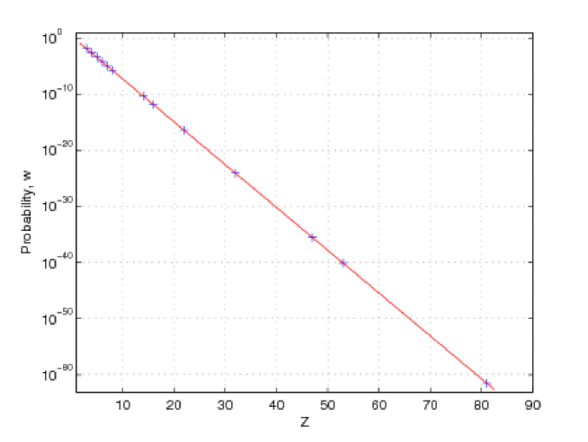
Figure 1: The probability for He to tunnel through the Coulomb potential barrier.

So for the lightest nuclei this probability is not negligible and for Li it is on the level of few percents and for Be only one order of magnitude smaller. It can provide a mechanism of anomalous isotope production, which challenges the search for such isotopes (e.g. for lithium $Li_{3}^{11+M_{X}}$).

Turning to the second case of emission of free He, let’s estimate the distance to the ”break point”, at which the potential energy $U(r)$ of Coulomb interaction with nucleus (with the account for screening by electron shells) becomes comparable with the binding energy $I_{0}$ of OHe, which can be determined from the condition

$$U(r)=\frac{I_{o}}{2}.$$

This distance for various atoms is represented on Fig. 2 in comparison with the radius of K-electron orbit of the atom.

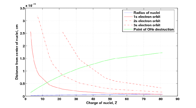
Figure 2: Comparision of the distance between break point of OHe and nucleus with its size and with K-electron orbit of the atom.

In particular for the iodine, this distance is of the order of

$$r_{b}=\frac{2Z_{1}Z_{2}\alpha}{I_{o}}=1.5\cdot 10^{-11}{\,\rm cm},$$ (68)

In most of the atoms it is situated somewhere between electron shells. However, as it has been shown on the figure, for light nuclei the break point is between the nucleus and K-electron orbit. It can lead to ionization of K-electron due to a perturbation of radial nuclear Coulomb field and appearance of a dipole component.

After breaking of the bound state, the both particles become free. Since $r_{b}\ll r_{at}$, where $r_{at}$ is the size of atom, X reaches the nucleus much quicker, than He leaves the atom. Therefore the first ionization of atom can happen due to the dipole perturbation of nuclear Coulomb field while He is present in the atom. However, as it is shown in the Appendix 2, this effect is negligible.

Immediate ionization is also possible due to the recoil momentum of the nucleus. It causes drastic displacement of the center of Coulomb field, what one can consider as a perturbation, which affects first of all on the K-electron. The probability of ionization for K-electron and electron from the last outer shell is estimated in Appendix 3. This estimation shows that even the outer electron can be emitted only in 1% cases. The probability of ionization of electrons from other levels is negligible. Therefore the contribution from this mechanism is not essential. Similar conclusion for the case of a WIMP-nucleus collision was obtained in a detailed analysis of Bernabei:2007jz

Then the X particle enters the nucleus and the electrons begin to feel the change of the Coulomb field. The nuclear charge decreases by two units when the Iodine ($I_{53}^{127}$) nucleus converts into anomalous Antimony ($Sb_{51}^{127+x}$), where $x$ is the mass of X in atomic mass units. Due to change of the binding energy, electron transitions with ionization and gamma ray emission take place. The above arguments show that immediate ionization, which would be inevitably masked by the large energy release from emitted He, is suppressed. The structure of electronic shells can changes in a long succession of atomic collisions, which can continue on scale up to $10^{-3}{\,\rm s}$. The following transitions (look at Fig. 3) will give rise to the signal in the range 2-6 keV. It refines the earlier arguments I2 ; KK2 .

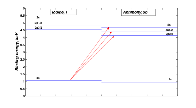
Figure 3: Energy levels of electron shells in Antimony and Iodine.

0.15.3 Ionization signal from OHe interaction in underground detectors

To calculate the cross section of the inelastic reaction (66) of $X^{--}$ capture by nucleus let’s determine the radius $R_{d}$, at which the field energy and the binding energy of OHe are equal:

$$\frac{Z_{X}Z_{nuc}\cdot\alpha}{R_{d}}\cdot\frac{R_{o}}{R_{d}}=I_{o}.$$

Here the radius of OHe $R_{o}$ is given by Eq.(59), its binding energy by Eq.(58), $Z_{nuc}$ - charge of initial nuclei (for example, for Iodine $Z_{nuc}=51$) and $Z_{X}=Z_{He}=2$ is the absolute value of charge of OHe components.

Then

$$R_{d}^{2}=\frac{2Z_{X}Z_{nuc}}{Z_{X}^{2}Z_{He}^{2}}\cdot\frac{1}{\alpha^{2}m_{He}^{2}}$$ (69)

For rough estimation of the cross section we’ll assume that the inelastic process is determined by exchange of X in $t$-channel. It gives a factor $(\frac{\Delta E}{m_{X}})^{2}$ in the probability of the process (66), where $\Delta E=I_{z}-I_{o}$ and $I_{z}>I_{o}$ is the binding energy of X in the nucleus. Then the cross section has the form

$$\sigma_{total}=\sigma_{d}\cdot(\frac{\Delta E}{m_{X}})^{2},$$ (70)

where $\sigma_{d}=\pi R_{d}^{2}$.

The relative probability for ionization signal in the range 2-6 keV, taking place with delay $>2\cdot 10^{-7}{\,\rm s}$ after emission of He is taken into account by factor $f$. The actual value of this factor is the subject of our further detailed analysis. Here we assume that it’s value is $0.01<f<0.1$.

Concentration of OHe in the matter of detector is given by (64) and velocity of particles in thermal equilibrium inside detector is $V_{nuc}=\sqrt{\frac{3kT}{m_{nuc}}}.$ For Iodine it equals $V/c=2.4\cdot 10^{-5}$ and for OHe $V/c=8.6\cdot 10^{-6}\cdot S_{3}^{-1/2}$.

So, the count rate in DAMA detector is

$$N_{CR}=N_{CR}^{(1)}+N_{CR}^{(2)}\cdot sin(\omega(t-t_{0}))$$ (71)

$$N_{CR}^{(i)}=fn_{oE}^{(i)}\cdot|{\overrightarrow{V_{OHe}}-\overrightarrow{V_{nuc}}}|\cdot\sigma_{total}\cdot\frac{N_{A}}{M},$$

where $i=1,2$. Then total amount of events during the time $t\gg 2\pi/\omega$ is determined by the constant part of the signal and is given by

$$N_{tot}=fn_{oE}^{(1)}\cdot|{\overrightarrow{V_{OHe}}-\overrightarrow{V_{nuc}}}|\cdot\sigma_{total}\cdot t\cdot\frac{N_{A}}{M},$$ (72)

where $N_{A}$ - Avogadro’s number,

$M$ - molar Iodine mass.

The part of dependence for the number of events per gramm per year on the mass of X with the amount of the events that corresponds to the observed amount of events 1.46 $\pm 3\sigma$ Bernabei:2008yi is given on Fig. 4 (for factor $f=0.1$ and $f=0.01$).

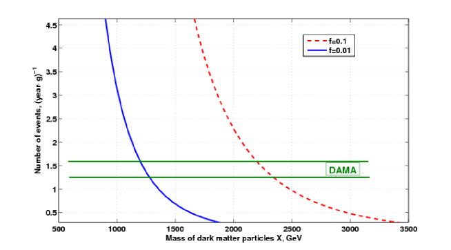
Figure 4: Dependence for number of events per gramm of Iodine per year of work from the dark matter particle mass (for $f=0.1$ and $0.01$).

Thus, at $0.01<f<0.1$ X particles with masses of about 1-2 TeV can explain the signal in DAMA experiment.

The Thallium concentration in NaI(Tl) detector is only 0.1 % from Iodine concentration DAMA_app , so the amount of events induced by OHe reaction with this element will be by 1000 times less. Therefore one can neglect the effects of such reaction with Thallium in the explanation of results from DAMA/NaI detector.

0.15.4 No signal in other detectors

The absence of the same result in other experiments (such as CDMS Akerib:2005kh ) can follow from the difference in their strategy.

For example in CDMS the working matter of detector is cooled down to the extralow temperature that leads to the suppression of the number of events (72) by two orders of magnitude. It was also shown in KK2 that nuclear recoil from reactions (66) in CDMS is below the threshold of registration while the effects of ionization, not accompanied by bolometric recoil are not considered as events CDMS_app .

Moreover this experiment is using semiconductor detectors. In these conditions the nuclei of atom are surely fixed in the knot of crystal lattice and electrons feel changing of the Coulomb potential very slow. So the probability of ionization has additional factor of suppression.

0.16 Conclusions

To conclude, the results of dark matter search in experiments DAMA/NaI and DAMA/LIBRA can find explanation in the framework of composite dark matter scenario without contradiction with negative results of other groups. This scenario can be realized in different frameworks, in particular in Minimal Walking Technicolor model or in the approach unifying spin and charges and contains distinct features, by which the present explanation can be distinguished from other recent approaches to this problem Edward (see also review and more references in Gelmini ).

The mechanisms of ionization induced by OHe reactions with nuclei were considered. It is argued that if in result of OHe interaction with matter of DAMA detector, the energy release in ionization comes in the range of 2-6 keV with sufficient delay, it can be distinguished from from immediate large energy release due to X capture by nucleus. Quantitative analysis of this explanation implies detailed study of a possibility for delayed transitions in atoms, perturbed by a rapid change of the charge of nucleus. An analogy with rearrangement of atomic shells after $\alpha$ decay of nucleus might be helpful in this analysis.

OHe concentration in matter of underground detectors follows the change in the incoming cosmic flux with the relaxation time of few minutes. It leads to annual modulations of the ionization signal from OHe reactions.

The method to calculate the rate of OHe reactions was developed and the calculated total amount of such events can to be consistent with the results of DAMA/NaI and DAMA/LIBRA experiments for the mass of OHe around 2 TeV. This method can be applied to the analysis of the whole set of inelastic processes, induced by O-helium in matter.

An inevitable consequence of the proposed explanation is appearance in the matter of DAMA/NaI or DAMA/LIBRA detector anomalous superheavy isotopes of antinomy (Sb with nuclear charge $Z=53-2=51$) and $10^{3}$ smaller amount of anomalous gold (Au with nuclear charge $Z=81-2=79$), created in the inelastic process (66) and having the mass roughly by $m_{o}$ larger, than ordinary isotopes of these elements. If the atoms of these anomalous isotopes are not completely ionized, their mobility is determined by atomic cross sections and becomes about 9 orders of magnitude smaller, than for O-helium. It provides conservation in the matter of detector of at least 200 anomalous atoms per 1g, corresponding to the number of events, observed in DAMA experiment. Therefore mass-spectroscopic analysis of this matter can provide additional test for the O-helium nature of DAMA signal. Similar mechanism can lead to presence of anomalous magnesium and zinc in the matter of CDMS detector.

An interesting aspect of our results is the challenging possibility of creation of anomalous isotopes of light elements like anomalous lithium $Li_{3}^{11+M_{X}}$ (from usual Li bound with OHe and from B bound with X), and of anomalous hydrogen $H_{1}^{7+M_{X}}$ (from lithium bound with X).

Appendix 1

The potential barrier of nucleus is presented on Fig. 5,where $T_{\alpha}$ - kinetic energy of $\alpha$-particle inside OHe, $r_{0}$ - characteristic distance of feeling the Coulomb barrier, R - radius of nuclei.

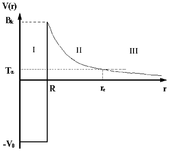
Figure 5: Coulomb barrier of the nucleus.

The height of this barrier $B_{k}$ is given by

$$B_{k}=\frac{Z_{1}Z_{2}\alpha}{r_{0}A^{\frac{1}{3}}}$$

and equal to 20.9 MeV for Iodine.

After the destruction of OHe, kinetic energy of helium equals to the binding energy of OHe state, which we take $I_{o}=1.289MeV$ with the account for charge distribution in He Pospelov . Effect of nonzero velocity of OHe before destruction is only 0.1% and can be neglected.

The probability of tunneling through the Coulomb barrier is given by the formula

$$w\sim exp(\frac{-2}{\hbar}\cdot\int_{R}^{r_{0}}\sqrt{2m(U(r)-T_{He})}dr)$$ (73)

where $\alpha=B_{k}\cdot R$. In case of potential $U(r)\sim\frac{\alpha}{r}$ the integral is equal to

$$w\sim exp(-\frac{2\alpha}{\hbar}\sqrt{\frac{2m}{T_{He}}}[arccos(\sqrt{\frac{T_{He}\cdot r_{e}}{\alpha}}-\sqrt{\frac{T_{He}\cdot r_{e}}{\alpha}(1-\frac{T_{He}\cdot r_{e}}{\alpha})})])$$

and the probability is

$$w\sim exp(-40)\ll 1.$$

Appendix 2

Effect of instantaneous ionization of atomic K-electron after $X^{--}$ is captured by nucleus in reaction (66) is similar to the same effect during $\alpha$-decay of a nucleus. Velocity of the $\alpha$-particle is negligible as compared with the velocity of K-electron, however the time, that it spend to leave the nucleus, is negligible as compared with the period of electron orbit rotation.

Perturbation that produces ionization in this case is the deviation of the combined nucleus and $\alpha$-particle field from ordinary Coulomb field 1/r. In the result of this deviation appears dipole momentum. On the other hand, the perturbation is efficient only during the period, when $\alpha$-particle is at small distances from the nucleus.

The initial state of the system is $(A+M+m,Z)=(A_{0},Z)$, then the final state of the system is $[(A+M,Z-q);(m,q)]=[(A_{1},Z-q);(m,q)]$, where $q$ and $m$ are the charge and mass of He, $Z$ and $A$ are the charge and mass of nucleus and $M$ is the mass of X.

Dipole momentum equals to

$$P=\frac{qA_{1}-(Z-q)m}{A_{0}}r_{0},$$ (74)

where $\overrightarrow{r_{0}}=\overrightarrow{r}_{nuclear}-\overrightarrow{r_{\alpha}}=\overrightarrow{V}t$ is the relative radius-vector of the nucleus and He and $\overrightarrow{V}$ - relative velocity.

Dipole component of the field is given by

$$V=\frac{P\overrightarrow{z}}{r^{3}}.$$

Here $\overrightarrow{z}$ is the direction along the velocity $\overrightarrow{V}$.

This component causes a perturbation for the electron on the orbit. According to perturbation theory the probability of the transition is determined by the matrix element of the transition from state 0 to the state with momentum k.

$$V_{0k}=\int\psi_{k}^{*}V\psi_{0}dq=P\int\psi_{k}^{*}(\frac{z}{r^{3}})\psi_{0}dq$$ (75)

The equation of motion of the electron on the shell reads as

$$\ddot{z}=-\frac{Zz}{r^{3}}.$$

Then

$$V_{0k}=P\int\psi_{k}^{*}(\ddot{z})\psi_{0}dq=P\frac{(E-E_{0})^{2}}{Z}z_{0k}$$

The probability for emission of electron from the shell to all the finite states is given by

$$\frac{dw}{dk}=2|\int V_{0k}e^{i(E_{0}-E)t}dt|^{2}=$$

$$=2|\int(\frac{qA_{1}-(Z-q)m}{A_{0}})\overrightarrow{V}t\frac{(E-E_{0})^{2}}{Z}z_{0k}e^{i(E-E_{0})t}dt|^{2}$$ (76)

With the use of a new multiplier $e^{-\lambda t}$, the integral is two taken times by parts. Then the integral from the imaginary exponent is taken and $\lambda\rightarrow 0$.

Thus

$$\frac{dw}{dk}=\frac{1}{\pi}(\frac{qA_{1}-(Z-q)m}{A_{0}Z})^{2}|z_{0k}|^{2}$$ (77)

Since the mass of the X $M\gg m$ the result is reduced to

$$\frac{dw}{dk}=\frac{1}{\pi}(\frac{qA_{1}}{A_{0}Z})^{2}|z_{0k}|^{2}.$$ (78)

Here $z_{0k}$ can be calculated if one takes into account that $z=rcos(\theta)$. Then

$$|z_{0k}|^{2}=|r_{0k}|^{2}|cos(\theta)_{0k}|^{2}=\frac{1}{3}|r_{0k}|^{2},$$

where $|r_{0k}|^{2}$ could be calculated owing to radial function $R_{k0}$

$$R_{k0}=\frac{2}{k^{2}}\sqrt{\frac{k!}{(k-1)!}}e^{-\frac{r}{k}}F(-k+1,2,r)=\frac{2}{k\sqrt{k}}e^{-\frac{r}{k}}F(-k+1,2,r)$$

Function $F$ could be found from the integral

$$J_{\alpha\gamma}^{\nu}=\int_{0}^{\infty}e^{-\lambda z}z^{\nu}F(\alpha,\gamma,kz)dz,$$ (79)

where one can find J as

$$J_{\alpha\gamma}^{\gamma+n-1}=(-1)^{n}\Gamma(\gamma)\frac{d^{n}}{d\lambda^{n}}[\lambda^{\alpha-\gamma}(\lambda-k)^{-\alpha}]$$ (80)

In our case $\alpha=-k+1;\gamma=2;kz=r$.

In the result the final answer reads as

$$dw=\frac{2^{11}(A_{1}-2Z+4)^{2}V^{2}}{3A_{0}^{2}Z^{6}(1+(\frac{k}{Z})^{2})^{5}}\frac{1}{1-e^{\frac{2\pi Z}{k}}}e^{-4\frac{Zarctg(\frac{k}{Z})}{k}}$$ (81)

In the limit of $M\rightarrow 0$ this result is transformed to the result, given in LL3 .

The probability distribution for K-electron ionization for Iodine and Natrium are presented correspondingly on Fig. 6(a) and (b) in the assumption that He leaves the nucleus with the velocity equal to 1/137).

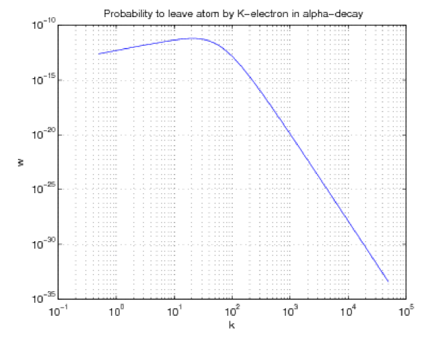
(a)

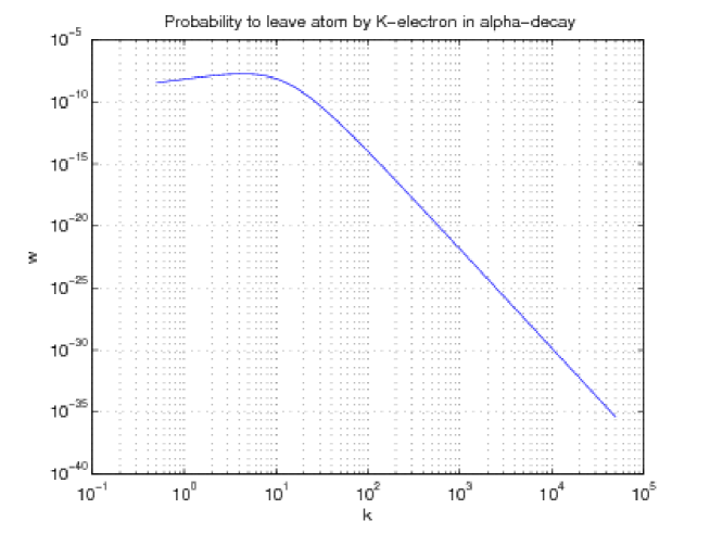
(b)

Figure 6: (a): Probability of the leaving Iodine atom by K-electron in the studying process. (b): Probability of the leaving Natrium atom by K-electron in the studying process.

The probabilities of K-electron emission from atoms of Iodine and Natrium are equal to $2\cdot 10^{-10}$ and $1.5\cdot 10^{-7}$, respectively. Therefore the considered mechanism of ionization is not effective.

Appendix 3

The probability of excitation and ionization of atom, when nucleus acquires recoil momentum and obtains velocity V.

The expansion of final wave functions through the initial ones is in the form $\psi^{{}^{\prime}}=\psi e^{-iq\sum r_{a}},$ where $q$ is momentum of the recoil nucleus and $r_{a}$ is radius-vector of electrons.

So probability of the transition is:

$$w_{k0}=|<k|e^{-iq\sum r_{a}}|0>|^{2}=1-w_{00}=1-|\int\psi^{2}e^{-iq\sum r_{a}}dV|^{2}$$ (82)

The integral can be taken analytically in the approximation $qr_{n}<<1$ for the wave functions from hydrogen atom.

Then

$$w_{k0}=1-\frac{1}{(1+\frac{1}{4}q^{2}r_{n}^{2})^{4}},$$ (83)

where $a$ is a radius of the considered electron shell,

$$\left\{\begin{aligned} \frac{m(V_{n}^{e})^{2}}{2}=I_{n}\\ mV_{n}^{e}r_{n}=n\hbar\\ \end{aligned}\right.$$

$\varepsilon$ is the binding energy of the electron on shell n and

$V_{n}^{e}$ is its velocity.

The radius of the electron shell is equal to

$$r_{n}=\frac{\hbar}{\sqrt{2mI_{n}}}.$$ (84)

Then

$$qr_{n}=\frac{mV_{nuc}}{\hbar}\cdot\frac{\hbar}{\sqrt{2m\varepsilon_{n}}}=\sqrt{\frac{m}{2\varepsilon_{n}}}V_{nuc}$$ (85)

The probability of ionization for K-electron and electron from the last outer shell are given in table.

Antimony $Sb_{51}^{127}$	$qa$	w
1s	$1.8\cdot 10^{-3}$	$3.5\cdot 10^{-6}$
5p	0.109	0.01

D. Lukman¹, N.S. Mankoč Borštnik¹ and H. B. Nielsen² Spin Connection Makes Massless Spinor Chirally Coupled to Kaluza-Klein Gauge Field After Compactification of $M^{1+5}$ to $M^{1+3}\times$ Infinite Disc Curved on $S^{2}$

0.17 Introduction

Kaluza-Klein-like theories, which are extremely elegant in the unification of all the interactions, have difficulties with masslessness of spinors after the compactification of some of the dimensions. The Approach unifying spins and charges (proposed by one of us—S.N.M.B.) is a Kaluza-Klein-like theory snmb1:norma92 ; snmb1:norma93 ; snmb1:norma94 ; snmb1:norma95 ; snmb1:Portoroz03 ; snmb1:pikanorma06 ; snmb1:gmdn06 ; snmb1:gmdn07 , which is besides unifying spins and charges into only the spin offering also the mechanism for generating families. This approach can be accepted as the theory showing a new way beyond the Standard model of the electroweak and colour interactions only after solving many open problems, among which is also the problem of the masslessness of spinors after the break of the starting symmetry in $d=(1+(d-1))$, $d\geq 14$ up to the symmetry assumed by the Standard model before the break of the electroweak symmetry in $d=(1+3)$.

Some of the open problems, common to all the Kaluza-Klein-like theories, are discussed in the paper of Witten snmb1:witten within the eleven-dimensional supergravity in a transparent way, leaving a strong impression that there is no hope, that the Kaluza-Klein-like theories can ever lead to the ”realistic” (observable) theory, since there is almost no hope for masslessness of quarks and leptons at the low energy level and no hope for the appearance of families. Many an open question of the Kaluza-Klein-like theories stays open also in other theories, like in theories of membranes, which assume that the dimension of space is more than 1+3. The question of masslessness of spinors at low energies as well as the appearance of families is also in these theories a hard not yet solved problem.

One of us is trying for long to develop the Approach unifying spins and charges so that spinors which carry in $d\geq 4$ nothing but two kinds of the spin (no charges), would manifest in $d=(1+3)$ all the properties assumed by the Standard model. The Approach proposes in $d=(1+(d-1))$ a simple starting action for spinors with the two kinds of the spin generators: the Dirac one, which takes care of the spin and the charges, and the second one, anticommuting with the Dirac one, which generates families . A spinor couples in $d=1+13$ to only the vielbeins and (through two kinds of the spin generators to) the spin connection fields. Appropriate breaks of the starting symmetry lead to the left handed quarks and leptons in $d=(1+3)$, which carry the weak charge while the right handed ones are weak chargeless. The Approach might have the right answer to the questions about the origin of families of quarks and leptons, about the explicit values of their masses and mixing matrices as well as about the masses of the scalar and the weak gauge fields, about the dark matter candidates, and about the break of the discrete symmetries.

In the refs. snmb1:hnkk06 ; snmb1:hn07 we demonstrated that the appropriate boundary condition ensures that a Weyl spinor in $d=(1+5)$ stays massless after the break of the starting symmetry to the symmetry of the flat disc with the boundary and the $(1+3)$ space, carrying one charge only  and coupling chirally to the corresponding gauge fields.

In this paper we study a similar toy model as in the refs. snmb1:hnkk06 ; snmb1:hn07 : a Weyl spinor in $d=(1+5)$, which breaks into $M^{1+3}$ and this time to an infinite disc, which the zweibein curves into $S^{2}$, while the chosen spin connection field allows on $S^{2}$ only one massless state of only one charge, since for this spin the spin connection field and the zweibein cancel each other. Then the charge of the massless spinor couples it to the corresponding gauge field. In $d=2$ the spin connection field and the zweibein (with no spinor sources) namely decouple from each other (there are not enough indices to make them coupled snmb1:dhnproc04 ; snmb1:deser95 ).

We take (as we did in ref. snmb1:hnkk06 ; snmb1:hn07 ) for the covariant momentum of a spinor

$$p_{0a} = f^{\alpha}{\!}_{a}p_{0\alpha},\quad p_{0\alpha}\psi=p_{\alpha}-\frac{1}{2}S^{cd}\omega_{cd\alpha}.$$ (86)

A spinor carries in $d\geq 4$ nothing but a spin and interacts accordingly with only the gauge fields of the corresponding generators of the infinitesimal transformations (of translations and the Lorentz transformations in the space of spinors), that is with vielbeins $f^{\alpha}{\!}_{a}$ and spin connections $\omega_{ab\alpha}$ (the gauge fields of $S^{ab}=\frac{i}{4}(\gamma^{a}\gamma^{b}-\gamma^{b}\gamma^{a})$). The corresponding Lagrange density for a Weyl spinor has the form ${\cal L}_{W}=\frac{1}{2}[(\psi^{\dagger}E\gamma^{0}\gamma^{a}p_{0a}\psi)+(\psi^{\dagger}E\gamma^{0}\gamma^{a}p_{0a}\psi)^{\dagger}]$, leading to

$${\cal L}_{W} = \psi^{\dagger}\gamma^{0}\gamma^{a}E\{f^{\alpha}_{a}p_{\alpha}+\frac{1}{2E}\{p_{\alpha},f^{\alpha}_{a}E\}_{-}-\frac{1}{2}S^{cd}\omega_{cda})\}\psi,$$ (87)

with $E=\det(e^{a}{\!}_{\alpha}),$ where

$$\omega_{cda} = \Re e\;\omega_{cda},\;\;{\rm if\;\;c,d,a\;\;all\;\;different}$$ (88)

$$= i\,\Im m\;\omega_{cda},\;\;\rm{otherwise}.$$

Let us have no gravity in $d=(1+3)$ ($f^{\mu}_{m}=\delta^{\mu}_{m}$ and $\omega_{mn\mu}=0$ for $m,n=0,1,2,3,\mu=0,1,2,3$) and let us make a choice of a zweibein on our disc (a two dimensional infinite plane with the rotational symmetry around the axes perpendicular to the plane)

$$e^{s}{}_{\sigma}=f^{-1}\begin{pmatrix}1&0\\ 0&1\end{pmatrix},f^{\sigma}{}_{s}=f\begin{pmatrix}1&0\\ 0&1\end{pmatrix},$$ (89)

with

$$f = 1+(\frac{\rho}{2\rho_{0}})^{2}=\frac{2}{1+\cos\vartheta},$$

$$x^{5} = \rho\,\cos\phi,\quad x^{6}=\rho\,\sin\phi,\quad E=f^{-2}.$$ (90)

The last relation follows from $ds^{2}=e_{s\sigma}e^{s}{\!}_{\tau}dx^{\sigma}dx^{\tau}=f^{-2}(d\rho^{2}+\rho^{2}d\phi^{2})$. The zweibein curves the infinite disc on the $S^{2}$ sphere with the radius $\rho_{0}$. We make a choice of the spin connection field

$$\omega_{st\sigma} = i\varepsilon_{st}\;\frac{4Fx_{\sigma}}{\rho}\frac{f-1}{\rho f}=-i\varepsilon_{st}\,\frac{F\,\sin\vartheta}{\rho_{0}}\,(\cos\phi,\sin\phi),\>s=5,6,\;\sigma=(5),(6),$$

which for the choice $0<2F\leq 1$ allows only one massless spinor of a particular charge on $S^{2}$, as we shall see in sect. 0.18. In the particular case that $2F=1$ the spin connection term $-S^{56}\omega_{56\sigma}$ compensates the term $\frac{1}{2Ef}\{p_{\sigma},Ef\}_{-}$ for the left handed spinor with respect to $d=1+3$, while for the spinor of the opposite handedness the spin connection term doubles the term $\frac{1}{2Ef}\{p_{\sigma},Ef\}_{-}$. $\phi$ determines the angle of rotations around the axis through the two poles of a sphere, while $\rho=2\rho_{0}\,\sqrt{\frac{1-\cos\vartheta}{1+\cos\vartheta}}$, where $\tan\frac{\vartheta}{2}=\frac{\rho}{2\rho_{0}}$, as can be read on Fig. 7. We shall see in sect. 0.18 that in the presence of the spin connection field from Eq.(LABEL:snmb1:omegas) the covariant derivative $\frac{\partial}{\partial\phi}$, becomes $\frac{\partial}{\partial\phi}-2iF(1-\cos\vartheta)$.

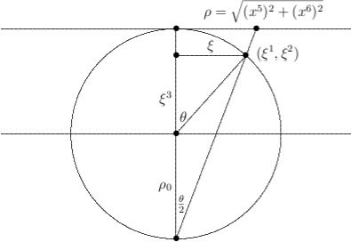
Figure 7: The disc is curved on the sphere $S^{2}$.

Such a choice of vielbeins and spin connection fields manifests the isometry, which leaves the form of the fields on $S^{2}$ unchanged. The infinitesimal coordinate transformations manifesting this symmetry are: $x^{{}^{\prime}\mu}=x^{\mu},$ $x^{{}^{\prime}\sigma}=x^{\sigma}+\phi_{A}\,K^{A\sigma}$, with $\phi_{A}$ the parameter of rotations around the axis which goes through both poles and with the infinitesimal generators of rotations around this axis $M^{(5)(6)}(=x^{(5)}p^{(6)}-x^{(6)}p^{(5)}+S^{(5)(6)})$

$$K^{A\sigma}=K^{(56)\sigma}=-iM^{(5)(6)}x^{\sigma}=\varepsilon^{\sigma}{}_{\tau}x^{\tau},$$ (92)

with $\varepsilon^{\sigma}{}_{\tau}=-1=-\varepsilon_{\tau}{}^{\sigma},\,\varepsilon^{(5)(6)}=1.$ The operators $K^{A}_{\sigma}=f^{-2}\varepsilon_{\sigma\tau}x^{\tau}$ fulfil the Killing relation

$$K^{A}_{\sigma,\tau}+\Gamma^{\sigma^{\prime}}{}_{\sigma\tau}K^{A}_{\sigma^{\prime}}+K^{A}_{\tau,\sigma}+\Gamma^{\sigma^{\prime}}{}_{\tau\sigma}K^{A}_{\sigma^{\prime}}=0$$

(with $\Gamma^{\sigma^{\prime}}{}_{\sigma\tau}=-\frac{1}{2}\,g^{\rho\sigma^{\prime}}(g_{\tau\rho,\sigma}+g_{\sigma\rho,\tau}-g_{\sigma\tau,\rho})$).

The equations of motion for spinors (the Weyl equations) which follow from the Lagrange density (Eq.87) are then

$$\{E\gamma^{0}\gamma^{m}p_{m}+Ef\gamma^{0}\gamma^{s}\delta^{\sigma}_{s}(p_{0\sigma}+\frac{1}{2Ef}\{p_{\sigma},Ef\}_{-})\}\psi=0,\quad{\rm with}$$

$$p_{0\sigma}=p_{\sigma}-\frac{1}{2}S^{st}\omega_{st\sigma},$$ (93)

with $f$ from Eq.(0.17) and with $\omega_{st\sigma}$ from Eq.(LABEL:snmb1:omegas). Taking into account that

$$\gamma^{a}p_{0a}\gamma^{b}p_{0b}=p_{0a}p_{0}{}^{a}-iS^{ab}S^{cd}\,{\cal R}_{abcd}+S^{ab}\,{\cal T}^{\beta}{}_{ab}\,p_{0\beta}$$

we find for the Riemann tensor and the torsion

$${\cal R}_{abcd}=f^{\alpha}_{[a}f^{\beta}_{b]}(\omega_{cd\beta,\alpha}-\omega_{ce\alpha}\omega^{e}{}_{d\beta}),$$

$${\cal T}^{\beta}{}_{ab}=f^{\alpha}_{[a}(f^{\beta}_{b]})_{,\alpha}+\omega_{[a}{}^{c}{}_{b]}f^{\beta}_{c}.$$ (94)

$[a\,\,b]$ means the antisymmetrization over the two indices $a$ and $b$. From Eq.(94) we read that to the torsion on $S^{2}$ both, the zweibein $f^{\sigma}_{\tau}$ and the spin connection $\omega_{st\sigma}$, contribute. While we have on $S^{2}$ for ${\cal R}_{\sigma\tau}=f^{-2}\eta_{\sigma\tau}\frac{1}{\rho^{2}}$ and correspondingly for the curvature ${\cal R}=\frac{-2}{(\rho_{0})^{2}}$, we find for the torsion ${\cal T}^{s}{}_{ts^{\prime}}={\cal T}^{s}{}_{t\sigma}f^{\sigma}_{s^{\prime}}$ with ${\cal T}^{5}{}_{ss}=0={\cal T}^{6}{}_{ss},\quad s=5,6,$ ${\cal T}^{5}{}_{65}=-{\cal T}^{5}{}_{56}=-(f_{,6}+\frac{4iF(f-1)}{\rho^{2}}x_{5}),$ ${\cal T}^{6}{}_{56}=-{\cal T}^{6}{}_{65}=-f_{,5}+\frac{4iF(f-1)}{\rho^{2}}x_{6}.$ The torsion ${\cal T}^{2}={\cal T}^{s}{}_{ts^{\prime}}{\cal T}_{s}{}^{ts^{\prime}}$ is for our particular choice of the zweibein and spin connection fields from Eq.87 correspondingly equal to $-\frac{2\rho^{2}}{(\rho_{0})^{4}}(1-(2F)^{2})$ (which is for the choice $2F=1$ equal to zero.).

We assume that the action for the gravitational field (which could hopefully give the desired solutions of equations of motion for the zweibein and the spin connection field in the presence of many spinor sources and what we have tried to find but with no success up to now) is linear in the Riemann scalar ${\cal R}={\cal R}_{abcd}\eta^{ac}\eta^{bd}$ and is in the lowest order with respect to the torsion ($\beta{\cal T}^{2}=\beta_{a}{\cal T}^{a}{}_{bc}{\cal T}_{a}{}^{bc}+\beta_{b}{\cal T}^{a}{}_{bc}{\cal T}^{b}{}_{a}{}^{c}+\beta_{c}{\cal T}^{a}{}_{ac}{\cal T}^{b}{}_{b}{}^{c}$) of Eq.94

$${\cal S}=\int\;d^{d}x\,(E\alpha{\cal R}+E\beta{\cal T}^{2}+{\cal L}_{W}).$$ (95)

The fermion part ${\cal L}_{W}$ is presented in Eq.(87) (and must include when searching for the desired spin connection and zweibein many spinors).

0.18 Equations of motion for spinors and the solutions

The equations of motion (93) for a spinor in $(1+5)$-dimensional space, which breaks into $M^{(1+3)}$ $\times S^{2}$, let the spinor ”feel” the zweibein $f^{\sigma}{\!}_{s}=\delta^{\sigma}{\!}_{s}f(\rho),\,f(\rho)=1+(\frac{\rho}{2\rho_{0}})^{2}=\frac{2}{1+\cos\vartheta}$ and the spin connection

$$\omega_{st\sigma}=4iF\varepsilon_{st}\frac{x_{\sigma}}{\rho}\,\frac{f-1}{\rho f}=iF\frac{\sin\vartheta}{\rho_{0}}\,(\cos\phi,\sin\phi).$$

The solution for a spinor in $d=(1+5)$ should be written as a superposition of all four ($2^{6/2-1}$) states of a single Weyl representation. (We kindly ask the reader to see the technical details about how to write a Weyl representation in terms of the Clifford algebra objects after making a choice of the Cartan subalgebra, for which we take: $S^{03},S^{12},S^{56}$ in the refs. snmb1:holgernorma2002 ; snmb1:hn07 . ) In our technique snmb1:holgernorma2002 one spinor representation—the four states, which all are the eigenstates of the chosen Cartan subalgebra—are the following four products of projections $\stackrel{{\scriptstyle ab}}{{[k]}}$ and nilpotents $\stackrel{{\scriptstyle ab}}{{(k)}}$:

$$\varphi^{1}_{1} = \stackrel{{\scriptstyle 56}}{{(+)}}\stackrel{{\scriptstyle 03}}{{(+i)}}\stackrel{{\scriptstyle 12}}{{(+)}}\psi_{0},$$

$$\varphi^{1}_{2} = \stackrel{{\scriptstyle 56}}{{(+)}}\stackrel{{\scriptstyle 03}}{{[-i]}}\stackrel{{\scriptstyle 12}}{{[-]}}\psi_{0},$$

$$\varphi^{2}_{1} = \stackrel{{\scriptstyle 56}}{{[-]}}\stackrel{{\scriptstyle 03}}{{[-i]}}\stackrel{{\scriptstyle 12}}{{(+)}}\psi_{0},$$

$$\varphi^{2}_{2} = \stackrel{{\scriptstyle 56}}{{[-]}}\stackrel{{\scriptstyle 03}}{{(+i)}}\stackrel{{\scriptstyle 12}}{{[-]}}\psi_{0},$$ (96)

where $\psi_{0}$ is a vacuum state. If we write the operators of handedness in $d=(1+5)$ as $\Gamma^{(1+5)}=\gamma^{0}\gamma^{1}\gamma^{2}\gamma^{3}\gamma^{5}\gamma^{6}$ ($=2^{3}iS^{03}S^{12}S^{56}$), in $d=(1+3)$ as $\Gamma^{(1+3)}=-i\gamma^{0}\gamma^{1}\gamma^{2}\gamma^{3}$ ($=2^{2}iS^{03}S^{12}$) and in the two dimensional space as $\Gamma^{(2)}=i\gamma^{5}\gamma^{6}$ ($=2S^{56}$), we find that all four states are left handed with respect to $\Gamma^{(1+5)}$, with the eigenvalue $-1$, the first two states are right handed and the second two states are left handed with respect to $\Gamma^{(2)}$, with the eigenvalues $1$ and $-1$, respectively, while the first two are left handed and the second two right handed with respect to $\Gamma^{(1+3)}$ with the eigenvalues $-1$ and $1$, respectively. Taking into account Eq.(96) we may write snmb1:hn07 the most general wave function $\psi^{(6)}$ obeying Eq.(93) in $d=(1+5)$ as

$$\psi^{(6)}={\cal A}\,{\stackrel{{\scriptstyle 56}}{{(+)}}}\,\psi^{(4)}_{(+)}+{\cal B}\,{\stackrel{{\scriptstyle 56}}{{[-]}}}\,\psi^{(4)}_{(-)},$$ (97)

where ${\cal A}$ and ${\cal B}$ depend on $x^{\sigma}$, while $\psi^{(4)}_{(+)}$ and $\psi^{(4)}_{(-)}$ determine the spin and the coordinate dependent parts of the wave function $\psi^{(6)}$ in $d=(1+3)$

$$\psi^{(4)}_{(+)} = \alpha_{+}\;{\stackrel{{\scriptstyle 03}}{{(+i)}}}\,{\stackrel{{\scriptstyle 12}}{{(+)}}}+\beta_{+}\;{\stackrel{{\scriptstyle 03}}{{[-i]}}}\,{\stackrel{{\scriptstyle 12}}{{[-]}}},$$

$$\psi^{(4)}_{(-)} = \alpha_{-}\;{\stackrel{{\scriptstyle 03}}{{[-i]}}}\,{\stackrel{{\scriptstyle 12}}{{(+)}}}+\beta_{-}\;{\stackrel{{\scriptstyle 03}}{{(+i)}}}\,{\stackrel{{\scriptstyle 12}}{{[-]}}}.$$ (98)

Using $\psi^{(6)}$ in Eq.(93) we recognize the following expressions as the mass terms: $\frac{\alpha_{+}}{\alpha_{-}}(p^{0}-p^{3})-\frac{\beta_{+}}{\alpha_{-}}(p^{1}-ip^{2})=m,$ $\frac{\beta_{+}}{\beta_{-}}(p^{0}+p^{3})-\frac{\alpha_{+}}{\beta_{-}}(p^{1}+ip^{2})=m,$ $\frac{\alpha_{-}}{\alpha_{+}}(p^{0}+p^{3})+\frac{\beta_{-}}{\alpha_{+}}(p^{1}-ip^{2})=m,$ $\frac{\beta_{-}}{\beta_{+}}(p^{0}-p^{3})+\frac{\alpha_{-}}{\beta_{+}}(p^{1}-ip^{2})=m.$ (One can notice that for massless solutions ($m=0$) the $\psi^{(4)}_{(+)}$ and $\psi^{(4)}_{(-)}$ decouple.) Taking into account that $S^{56}\stackrel{{\scriptstyle 56}}{{(+)}}=\frac{1}{2}\stackrel{{\scriptstyle 56}}{{(+)}}$, while $S^{56}\stackrel{{\scriptstyle 56}}{{[-]}}=-\frac{1}{2}\stackrel{{\scriptstyle 56}}{{[-]}}$, we end up with the equations of motion for ${\cal A}$ and ${\cal B}$ as follow

$$-2i\,f\,(\frac{\partial}{\partial z}+\frac{\partial\ln\sqrt{Ef}}{\partial z}-\frac{e^{-i\phi}}{\rho}G)\,{\cal B}+m\;{\cal A}=0,$$

$$-2i\,f\,(\frac{\partial}{\partial\bar{z}}+\frac{\partial\ln\sqrt{Ef}}{\partial\bar{z}}+\frac{e^{i\phi}}{\rho}G)\,{\cal A}+m\;{\cal B}=0,$$ (99)

where $z:=x^{5}+ix^{6}=\rho\,e^{i\phi}$, $\bar{z}:=x^{5}-ix^{6}=\rho\,e^{-i\phi}$ and $\frac{\partial}{\partial z}=\frac{1}{2}\,(\frac{\partial}{\partial x^{5}}-i\frac{\partial}{\partial x^{6}})=\frac{e^{-i\phi}}{2}\;(\frac{\partial}{\partial\rho}-\frac{i}{\rho}\,\frac{\partial}{\partial\phi})$, $\frac{\partial}{\partial\bar{z}}=\frac{1}{2}\,(\frac{\partial}{\partial x^{5}}+i\frac{\partial}{\partial x^{6}})=\frac{e^{i\phi}}{2}\;(\frac{\partial}{\partial\rho}+\frac{i}{\rho}\,\frac{\partial}{\partial\phi})$. Eq.(99) can be rewritten as follows

$$-if\,e^{-i\phi}\,(\frac{\partial}{\partial\rho}-\frac{i}{\rho}\,(\frac{\partial}{\partial\phi}-i2G)+\frac{\partial}{\partial\rho}\ln{\sqrt{Ef}}){\cal B}+m{\cal A}=0,$$

$$-if\,e^{i\phi}\,(\frac{\partial}{\partial\rho}+\frac{i}{\rho}\,(\frac{\partial}{\partial\phi}-i2G)+\frac{\partial}{\partial\rho}\ln{\sqrt{Ef}}){\cal A}+m{\cal B}=0,$$ (100)

with $G=4F\frac{f-1}{f}(=2F(1-\cos\vartheta))$. Having the rotational symmetry around the axis perpendicular to the plane of the fifth and the sixth dimension we require that $\psi^{(6)}$ is the eigenfunction of the total angular momentum operator $M^{56}$

$$M^{56}\psi^{(6)}=(n+\frac{1}{2})\,\psi^{(6)},\quad M^{56}=x^{5}p^{6}-x^{6}p^{5}+S^{56}.$$ (101)

Let ${\cal A}={\cal A}_{n}(\rho)\,\rho^{n}\,e^{in\phi}$ and ${\cal B}={\cal B}_{n}(\rho)\,\rho^{-n}\,e^{in\phi}$.

Let us treat first the massless case ($m=0$). Taking into account that $\frac{G}{\rho}=\frac{\partial}{\partial\rho}\ln f^{2F}$ and that $E=f^{-2}$ it follows

$$\frac{\partial\,\ln({\cal B}\,f^{-F-1/2})}{\partial\rho} = 0,$$

$$\frac{\partial\,\ln({\cal A}\,f^{F-1/2})}{\partial\rho} = 0.$$ (102)

We get correspondingly the solutions

$${\cal B}_{n} = {\cal B}_{0}\,e^{in\phi}\,\rho^{-n}f^{F+1/2},$$

$${\cal A}_{n} = {\cal A}_{0}\,e^{in\phi}\,\rho^{n}f^{-F+1/2}.$$ (103)

Requiring that only normalizable (square integrable) solutions are acceptable

$$2\pi\,\int^{\infty}_{0}\,E\,\rho d\rho{\cal A}^{\star}_{n}{\cal A}_{n} <\infty,$$

$$2\pi\,\int^{\infty}_{0}\,E\,\rho d\rho{\cal B}^{\star}_{n}{\cal B}_{n} <\infty,$$ (104)

it follows

$${\rm for}\;{\cal A}_{n}:-1<n<2F,$$

$${\rm for}\;{\cal B}_{n}:2F<n<1,\quad n\;\;{\rm is\;\;an\;\;integer}.$$ (105)

Eq.(105) tells us that the strength $F$ of the spin connection field $\omega_{56\sigma}$ can make a choice between the two massless solutions ${\cal A}_{n}$ and ${\cal B}_{n}$: For $0<2F\leq 1$ the only massless solution is the left handed spinor with respect to $(1+3)$

$$\psi^{(6)}_{0}={\cal N}_{0}f^{-F+1/2}\stackrel{{\scriptstyle 56}}{{(+)}}\psi^{(4)}_{(+)}.$$ (106)

It is the eigenfunction of $M^{56}$ with the eigenvalue $1/2$. No right handed solution is allowed for $0<2F\leq 1$. For the particular choice $2F=1$ the spin connection field $-S^{56}\omega_{56\sigma}$ compensates the term $\frac{1}{2Ef}\{p_{\sigma},Ef\}_{-}$ and the left handed spinor with respect to $d=1+3$ becomes a constant with respect to $\rho$ and $\phi$.

For $2F=1$ it is easy to find also all the massive solutions of Eq.(100). To see this let us rewrite Eq.(100) in terms of the parameter $\vartheta$. Taking into account that $f=\frac{2}{1+\cos\vartheta}$, $\omega_{56\sigma}=-iF\frac{\sin\vartheta}{\rho_{0}}\;(\cos\phi,\sin\phi)$ and assuming that ${\cal A}={\cal A}_{n}(\rho)\,e^{in\phi}$ and ${\cal B}={\cal B}_{n+1}(\rho)\,e^{i(n+1)\phi}$, which guarantees that the states will be the eigenstates of $M^{56}$, it follows

$$(\frac{\partial}{\partial\vartheta}+\frac{n+1-(F+1/2)(1-\cos\vartheta)}{\sin\vartheta}){\cal B}_{n+1}+i\tilde{m}{\cal A}_{n}=0,$$

$$(\frac{\partial}{\partial\vartheta}+\frac{-n+(F-1/2)(1-\cos\vartheta)}{\sin\vartheta}){\cal A}_{n}+i\tilde{m}{\cal B}_{n+1}=0,$$ (107)

with $\tilde{m}=\rho_{0}m$. For the particular choice of $2F=1$ the equations simplify to

$$(\frac{\partial}{\partial\vartheta}+\frac{n+\cos\vartheta}{\sin\vartheta}){\cal B}_{n+1}+i\tilde{m}{\cal A}_{n}=0,$$

$$(\frac{\partial}{\partial\vartheta}-\frac{n}{\sin\vartheta}){\cal A}_{n}+i\tilde{m}{\cal B}_{n+1}=0,$$ (108)

from where we obtain

$$\{\frac{1}{\sin{\vartheta}}\frac{\partial}{\partial\vartheta}(\sin{\vartheta}\frac{\partial}{\partial\vartheta})+[\tilde{m}^{2}+\frac{(-n^{2}-1-2n\cos\vartheta)}{\sin^{2}\vartheta}]\}{\cal B}_{n+1}=0,$$

$$\{\frac{1}{\sin\vartheta}\frac{\partial}{\partial\vartheta}(\sin\vartheta\frac{\partial}{\partial\vartheta})+[\tilde{m}^{2}-\frac{n^{2}}{\sin^{2}\vartheta}]\}{\cal A}_{n}=0.$$ (109)

From above equations we see that for $\tilde{m}=0$, that is for the massless case, the only solution with $n=0$ exists, which is $Y^{0}_{0}$, the spherical harmonics, which is a constant (in agreement with our discussions above). All the massive solutions have $\tilde{m}^{2}=l(l+1),\,l=1,2,3,..$ and $-l\leq n\leq l$. Legendre polynomials are the solutions for ${\cal A}_{n}=P^{l}_{n}$, as it can be read from the second of the equations Eq.(109), while we read from the second equation of Eq.(108) that

$${\cal B}_{n+1}=\frac{i}{\sqrt{l(l+1}}\,(\frac{\partial}{\partial\vartheta}-\frac{n}{\sin\vartheta})P^{l}_{n}.$$

Accordingly the massive solution with the mass equal to $m=l(l+1)/\rho_{0}$ (we use the units in which $c=1=\hbar$) and the eigenvalues of $M^{56}$ ((Eq.101))—which is the charge as we shall see later—equal to $(\frac{1}{2}+n)$, with $-l\leq n\leq l$, $l=1,2,..$, are

$$\psi^{(6)\tilde{m}^{2}=l(l+1)}_{n+1/2} = {\cal N}^{l}_{n+1/2}\{\stackrel{{\scriptstyle 56}}{{(+)}}\psi^{(4)}_{(+)}+\frac{i}{\sqrt{l(l+1)}}\,\stackrel{{\scriptstyle 56}}{{[-]}}\psi^{(4)}_{(-)}\,e^{i\phi}(\frac{\partial}{\partial\vartheta}\,-\frac{n}{\sin\vartheta})\}Y^{l}_{n})$$

with $Y^{l}_{n}$, which are the spherical harmonics. Rewriting the mass operator $\hat{m}=\gamma^{0}\gamma^{s}f^{\sigma}_{s}(p_{\sigma}-S^{56}\omega_{56\sigma}+\frac{1}{2Ef}\{p_{\sigma},Ef\}_{-})$ as a function of $\vartheta$ and $\phi$

$$\rho_{0}\hat{m} = i\gamma^{0}\,\{\stackrel{{\scriptstyle 56}}{{(+)}}e^{-i\phi}(\frac{\partial}{\partial\vartheta}\,-\frac{i}{\sin\vartheta}\frac{\partial}{\partial\phi}\,-\frac{1-\cos\vartheta}{\sin\vartheta})+\stackrel{{\scriptstyle 56}}{{(-)}}e^{i\phi}(\frac{\partial}{\partial\vartheta}\,+\frac{i}{\sin\vartheta}\frac{\partial}{\partial\phi})\},$$

(111)

one can easily show that when applying $\rho_{0}\hat{m}$ and $M^{56}$ on $\psi^{(6)\tilde{m}^{2}=k(k+1)}_{n+1/2}$, for $-k\leq n\leq k$, one obtains from Eq.(LABEL:snmb1:knsol)

$$\rho_{0}\hat{m}\,\psi^{(6)\tilde{m}^{2}=k(k+1)}_{n+1/2} = k(k+1)\psi^{(6)\tilde{m}^{2}=k(k+1)}_{n+1/2},$$

$$M^{56}\,\psi^{(6)\tilde{m}^{2}=(n+1/2)k(k+1)}_{n+1/2} = (n+1/2)\psi^{(6)\tilde{m}^{2}=k(k+1)}_{n+1/2}.$$ (112)

A wave packet, which is the eigen function of $M^{56}$ with the eigenvalue $1/2$, for example, can be written as

$$\psi^{(6)}_{1/2} = \sum_{k=0,\infty}C_{1/2}^{k}\;\,{\cal N}_{1/2}\{\stackrel{{\scriptstyle 56}}{{(+)}}\psi^{(4)}_{(+)}+(1-\delta^{k}_{0})\frac{i}{\sqrt{k(k+1)}}\,\stackrel{{\scriptstyle 56}}{{[-]}}\psi^{(4)}_{(-)}\,e^{i\phi}\frac{\partial}{\partial\vartheta}\}Y^{k}_{0}.$$

(113)

The expectation value of the mass operator $\hat{m}$ on such a wave packet is

$$\sum_{k=0,\infty}C_{1/2}^{k*}C_{1/2}^{k}\sqrt{k(k+1)}/\rho_{0}.$$

It remains to comment the meaning of the exclusion of the south pole on $S^{2}$, since the disc with the zweibein equal to $f=\frac{2}{1+\cos\vartheta}$ looks like $S^{2}$ up to the southern pole.

To start from the southern pole one must rewrite Eq.(108) and the second equation of Eq.(109) so that $\vartheta$ is replaced by $(\pi-\vartheta)$

$$(\frac{\partial}{\partial(\pi-\vartheta)}+\frac{-n+\cos(\pi-\vartheta)}{\sin(\pi-\vartheta)})(-){\cal B}_{-n+1}+i\tilde{m}{\cal A}_{-n}=0,$$

$$(\frac{\partial}{\partial(\pi-\vartheta)}-\frac{-n}{\sin\vartheta}){\cal A}_{-n}+i\tilde{m}(-){\cal B}_{-n+1}=0,$$ (114)

and

$$\{\frac{1}{\sin(\pi-\vartheta)}\frac{\partial}{\partial(\pi-\vartheta)}(\sin(\pi-\vartheta)\frac{\partial}{\partial(\pi-\vartheta)})+[\tilde{m}^{2}-\frac{(-n)^{2}}{\sin^{2}(\pi-\vartheta)}]\}{\cal A}_{-n}=0.$$

(115)

Since ${\cal A}_{-n}(\pi-\vartheta)=P^{l}_{-n}(\pi-\vartheta)=(-1)^{l+n}P^{l}_{n}(\vartheta)$ are the solutions of Eq.(115) and since $P^{l}_{-n}(\pi-\vartheta)=(-)^{l+2n}P^{l}_{n}(\theta)$, the solutions of Eq.(115) coincide with the solutions of Eq.(109). Correspondingly also the solutions for $(-){\cal B}_{-n+1}(\pi-\vartheta)=\frac{i}{\tilde{m}}(\frac{\partial}{\partial(\pi-\vartheta)}-\frac{-n}{\sin\vartheta}){\cal A}_{-n}(\pi-\vartheta)$ coincide with the solutions of ${\cal B}_{n+1}(\vartheta)$, which proves that the one missing point on $S^{2}$ makes no harm.

0.19 Spinors and the gauge fields in $d=(1+3)$

To study how do spinors couple to the Kaluza-Klein gauge fields in the case of $M^{(1+5)}$, “broken” to $M^{(1+3)}\times S^{2}$ with the radius of $S^{2}$ equal to $\rho_{0}$ and with the spin connection field $\omega_{st\sigma}=i4F\varepsilon_{st}\frac{x_{\sigma}}{\rho}\frac{f-1}{\rho f}$ we first look for (background) gauge gravitational fields, which preserve the rotational symmetry around the axis through the northern and southern pole. Requiring that the symmetry determined by the Killing vectors of Eq.(92) (following ref. snmb1:hnkk06 ) with $f^{\sigma}{}_{s}=f\delta^{\sigma}_{s},f^{\mu}{}_{s}=0,e^{s}{}_{\sigma}=f^{-1}\delta^{s}_{\sigma},e^{m}{}_{\sigma}=0,$ is preserved, we find for the background vielbein field

$$e^{a}{}_{\alpha}=\begin{pmatrix}\delta^{m}{}_{\mu}&e^{m}{}_{\sigma}=0\\ e^{s}{}_{\mu}&e^{s}{}_{\sigma}\end{pmatrix},f^{\alpha}{}_{a}=\begin{pmatrix}\delta^{\mu}{}_{m}&f^{\sigma}{}_{m}\\ 0=f^{\mu}{}_{s}&f^{\sigma}{}_{s}\end{pmatrix},$$ (116)

with

$$f^{\sigma}{}_{m} = K^{(56)\sigma}B^{(5)(6)}_{\mu}f^{\mu}{}_{m}=\varepsilon^{\sigma}{}_{\tau}x^{\tau}A_{\mu}\delta^{\mu}_{m},$$

$$e^{s}{}_{\mu} = -\varepsilon^{\sigma}{}_{\tau}x^{\tau}A_{\mu}e^{s}{}_{\sigma},$$ (117)

$s=5,6;\sigma=(5),(6)$. Requiring that correspondingly the only nonzero torsion fields are those from Eq.(94) we find for the spin connection fields

$$\omega_{st\mu}=\varepsilon_{st}A_{\mu},\quad\omega_{sm\mu}=\frac{1}{2}f^{-1}\varepsilon_{s\sigma}x^{\sigma}\delta^{\nu}{}_{m}F_{\mu\nu},$$ (118)

$F_{\mu\nu}=A_{[\nu,\mu]}$. The $U(1)$ gauge field $A_{\mu}$ depends only on $x^{\mu}$. All the other components of the spin connection fields, except (by the Killing symmetry preserved) $\omega_{st\sigma}$ from Eq.(93), are zero, since for simplicity we allow no gravity in $(1+3)$ dimensional space. The corresponding nonzero torsion fields ${\cal T}^{a}{}_{bc}$ are presented in Eq.(94), all the other components are zero.

To determine the current, which couples the spinor to the Kaluza-Klein gauge fields $A_{\mu}$, we analyze (as in the refs. snmb1:hnkk06 ; snmb1:hn07 ) the spinor action (Eq.(87))

$${\cal S} = \int\;d^{d}x\bar{\psi}^{(6)}E\gamma^{a}p_{0a}\psi^{(6)}=$$ (119)

$$\int\,d^{d}x\bar{\psi}^{(6)}\gamma^{s}p_{s}\psi^{(6)}+$$

$$\int\,d^{d}x\bar{\psi}^{(6)}\gamma^{m}\delta^{\mu}{}_{m}p_{\mu}\psi^{(6)}+$$

$$\int\,d^{d}x\bar{\psi}^{(6)}\gamma^{m}\delta^{\mu}{}_{m}A_{\mu}(\varepsilon^{\sigma}{}_{\tau}x^{\tau}p_{\sigma}+S^{56})\psi^{(6)}+$$

$${\rm\;terms}\propto x^{\sigma}\,{\rm or}\propto x^{5}x^{6}.$$

Here $\psi^{(6)}$ is a spinor state in $d=(1+5)$ after the break of $M^{1+5}$ into $M^{1+3}\times$ $S^{2}$. $E$ is for $f^{\alpha}{}_{a}$ from Eq.(116) equal to $f^{-2}$. The term in the second row in Eq.(119) is the mass term (equal to zero for the massless spinor), the term in the third row is the kinetic term, together with the term in the fourth row defines the covariant derivative $p_{0\mu}$ in $d=(1+3)$. The terms in the last row contribute nothing when the integration over the disk (curved into a sphere $S^{2}$) is performed, since they all are proportional to $x^{\sigma}$ or to $x^{5}x^{6}\;$ ($-\gamma^{m}\,\frac{1}{2}S^{sm}\omega_{smn}=-\gamma^{m}\,\frac{1}{2}\,f^{-1}F_{mn}\varepsilon_{s\sigma}x^{\sigma}$ and $-\gamma^{m}\,f^{\sigma}{}_{m}\frac{1}{2}\,S^{st}\omega_{st\sigma}=\gamma^{m}A_{m}x^{5}x^{6}S^{st}\varepsilon_{st}\frac{4iF(f-1)}{f\rho^{2}}$).

We end up with the current in $(1+3)$

$$j^{\mu}=\int\;Ed^{2}x\bar{\psi}^{(6)}\gamma^{m}\delta^{\mu}{}_{m}M^{56}\psi^{(6)}.$$ (120)

The charge in $d=(1+3)$ is proportional to the total angular momentum $M^{56}=L^{56}+S^{56}$ around the axis from the southern to the northern pole of $S^{2}$, but since for the choice of $2F=1$ (and for any $0<2F\leq 1$) in Eq.(105) only a left handed massless spinor exists, with the angular momentum zero, the charge of a massless spinor in $d=(1+3)$ is equal to $1/2$.

The Riemann scalar is for the vielbein of Eq.(116) equal to

$${\cal R}=-\frac{1}{2}\rho^{2}f^{-2}F^{mn}F_{mn}.$$

If we integrate the Riemann scalar over the fifth and the sixth dimension, we get $-\frac{8\pi}{3}(\rho_{0})^{4}F^{mn}F_{mn}$.

0.20 Conclusions

We presented in this letter a toy model of a left handed spinor carrying in $d=1+5$ nothing but a spin, with the symmetry of $M^{(1+5)}$, which breaks to $M^{(1+3)}\times$ the infinite disc with the zweibein, which curves the disc on $S^{2}$ ($f=1+(\frac{\rho}{2\rho_{0}})^{2}$, with $\rho_{0}$ the radius of $S^{2}$), and with the spin connection field on the disc equal to $\omega_{st\sigma}=\varepsilon_{st}\,i4F\frac{f-1}{\rho f}\frac{x_{\sigma}}{\rho},\sigma=(5),(6);s,t=5,6,$ which allows for $0<2F\leq 1$ one massless spinor of the charge $1/2$ and of the left handedness with respect to $d=(1+3)$. This spinor state couples chirally to the corresponding Kaluza-Klein gauge field. There are infinite many massive states, which are at the same time the eigenstates of $M^{56}=x^{5}p^{6}-x^{6}p^{5}+S^{56}$, with the eigen values $n+1/2$, carrying the Kaluza-Klein charge $n+1/2$. For the choice of $2F=1$ the massive states have the mass equal to $k(k+1)/\rho_{0},k=1,2,3,..$, with $-k\leq n\leq k$. We found the expression for the massless eigenstate and for the particular choice of $2F=1$ also for all the massive states.

We therefore found an example, in which the internal gauge fields—spin connections and zweibeins—allow only one massless state, that is the spinor of one handedness and of one charge with respect to $d=1+3$ space. Since for the zweibein curving the infinite disc on $S^{2}$, the spin connection field $\omega_{st\sigma}=i4F\frac{f-1}{\rho f}\frac{x_{\sigma}}{\rho},$ with any $2F$ fulfilling the condition $\;0<2F\leq 1$ ensures that a massless spinor state of only one handedness and one charge in $d=(1+3)$ exists (only one massless state is normalizable), it is not a fine tuning what we propose. To find simple solutions for the massive states, we made a choice of $2F=1$. The massless state is in this case a constant with respect to the two angles on $S^{2}$, while the angular dependence of the massive states, with the masses equal to $l(l+1)/\rho_{0}$, are expressible with the spherical harmonics $Y^{l}_{n},\;\;-l\leq n\leq l$, and with the $e^{i\phi}\,\frac{i}{\sqrt{l(l+1)}}\;(\frac{\partial}{\partial\vartheta}-\frac{i}{\sin\vartheta})Y^{l}_{n}$ (Eq.(LABEL:snmb1:knsol)).

We do not explain either how does the break of the $M^{(1+5)}$ to $M^{(1+3)}\times$ the infinite disc, with the zweibein which curves the disc on $S^{2}$, occur or what does make the spin connection field in the radial direction and of the strength, which allows spinors of only one handedness on $S^{2}$.

If the break of the starting symmetry $M^{1+5}$ occurs spontaneously because of the many body effects, like it is a many spinors state, then the spin connection field must be proportional to the number of spinors (it might be of different angular momentum each) and accordingly quantized. WE have tried to prove that such a spin connection field can occur due to the many body spinor functions, describing spinors in $d=1+5$. We could not found such a many body state. We even proved that such a field can not be generated by only spinors.

Let us conclude the paper by pointing out that while in the two papers snmb1:hnkk06 ; snmb1:hn07 we achieved the masslessness of a spinor, its mass protection and the chiral coupling to the corresponding Kaluza-Klein gauge field after a break of a symmetry from $d=1+5$ to $d=(1+3)$, with the choice of the boundary condition on a flat (finite) disk (without explaining where does such a boundary condition come from), in this letter the massless spinor and its chiral coupling to the corresponding Kaluza-Klein gauge field is achieved by the choice of the appropriate spin connection and zweibein fields (whose origin we were not able to derive).

We do not discuss the problem of the families in this paper. We kindly ask the reader to take a look on the refs. snmb1:norma92 ; snmb1:norma93 ; snmb1:norma94 ; snmb1:norma95 ; snmb1:Portoroz03 ; snmb1:pikanorma06 ; snmb1:gmdn06 ; snmb1:gmdn07 where the proposal for solving the problem of families is presented.

0.21 Acknowledgement

One of the authors (N.S.M.B.) would like to warmly thank Jože Vrabec for fruitful discussions.

R. Mirmansssbbg@gmail.com Some Obvious Matters of Physics That Are Not Obvious

0.22 Why we cannot expect gravitation to have weird properties

General relativity seems to have unphysical solutions like closed time-like curves, wormholes, … . This does not follow and is quite unlikely: the Einstein equation is a necessary condition for a gravitational field but not sufficient. There are additional requirements rm1ml and before we can conclude that there are fields with strange properties we must show that all conditions are satisfied. This is implausible for weird fields. Abnormal solutions imply that not all conditions are satisfied. And there are other problems.

These do not imply anything wrong with general relativity — it is almost certainly correct. It just means that it is applied incorrectly.

What are other conditions (rm1ml ; rm1bna ; rm1imp )?

The field must be produced, else it does not exist. What produces a gravitational field? A sphere, a star, dust? But there are no spheres, stars, dust. These are merely collections of protons, neutrons, electrons and such — which are what creates and is acted upon. Such a collection must give a strange field. However these objects are governed by quantum mechanics. The uncertainty principle applies. Can a collection of such objects produce strangeness? Before it is claimed that there are closed timelike curves, wormholes, …, it must be shown that there is a collection of quantum mechanical objects capable of producing them.

Would we expect a single proton, a single electron, to give closed timelike curves? If not why would we expect a collection to? This implies that the formalism is being used incorrectly. This can be tricky because we often think in ways different than the ones nature thinks in, like using classical physics as a formalism while nature uses quantum mechanics, or using large objects while nature produces gravitational fields from collections of quantum mechanical ones. Using the proper formalism is essential.

If such single objects, atoms and subsets, cannot form wormholes, or any other such strange things, then for them to be believed to exist it must be shown that sets of such elementary objects can give them. How many objects does it take? What determines this number? This does seem implausible does it not? The difficulty is that we take the source of the gravitational field as a macroscopic body, but there are none, only collections of electrons, protons and such. Hence we must either show that such objects are possible or conclude that they are purely the result of misuse of the formalism, like the use of macroscopic sources.

There is another condition which is especially interesting since it requires that general relativity be the theory of gravity (thus the quantum theory of gravity, as it so clearly is (rm1ml )). All properties of gravitation come from it. This has been discussed in depth, with all the mathematics shown and proven (rm1ml ; rm1bna ). Here we summarize.

A physical object, like a gravitational field, must be a representation basis state of the transformation group of geometry, the Poincaré group. (The Poincaré group is the transformation group, not the symmetry group, although it is interesting that it is the symmetry group also (rm1imp , sec. VI.2.a.ii, p. 113)).

To clarify consider the rotation group and an object with spin up. Its statefunction (a better term than wavefunction since nothing waves) gives the spin as up. A different observer sees the spin at some angle, thus a different statefunction. The statefunction of the first must be transformed to give that of the second. Thus for each set of coordinates there is a statefunction and these are transformed into each other when the coordinates are. For each rotation there is a transformation of the statefunction. Moreover the product of two transformations must correspond to the product of the two rotations that they go with. Also a rotation, being a group element, can be written as a product of two, or ten, or 1000, or in any of an infinite number of ways. Each such product has a product of transformations on the statefunction going with it, with each term in the product of transformations corresponding to a term in the product of rotations. Thus the transformations on the statefunction form a representation of the rotation group, and each statefunction generated from any one by such a transformation is a basis state of the rotation group representation.

This does not require that space or physics be invariant under the group. Rotations are a property of geometry whether space is invariant under them or not. Thus a state can be written as a sum of rotation basis states (spherical harmonics) and is taken into another such sum by a rotation. Each term in the latter is a sum of terms of the former (with coefficients functions of the angles). Each term is a sum only of terms from the same representation (states of angular momentum 1 go only into states of angular momentum 1, and so on). This is true whether space is invariant under rotations or not (say there is a direction, simulated by the vertical, that is different). An up state may with time go into a down one, but that is irrelevant since these (mathematical) transformations are considered at a single time. Also no matter how badly symmetry is broken there cannot be an object with spin-${1\over 3}$ or $\pi$. These would not be true if we expanded in unitary group states. The rotation group is a property of our (real) geometry.

It is only a subgroup. The transformation group of space thus of the fields is the Poincaré group. Statefunctions (including those of gravity, the connections) must be basis states of it. The Poincaré group is an inhomogeneous group so very different from the simple rotation group. Gravitation is massless. The entire analysis depends on this.

Massless and massive representations are much different. The little group of massive representations is semisimple (the rotation group), while that of massless ones is solvable. Thus massless objects have difficulty in coupling to massive ones. There are only three that can. Scalars apparently can. Helicity 1 gives electromagnetism (with its properties completely determined). For helicity 2 the indices do not match. Fortunately the formalism gives a nonlinear condition, the Bianchi identities, that allow gravitation to interact with massive objects. Gravitation must be nonlinear else it could not couple, so could not exist. Einstein’s equation then follows from the formalism, but is not all of it.

A supposed gravitational field must be shown to form a representation basis state of a massless helicity-2 representation of the Poincaré group or it is not a gravitational field. Unless ones with strange properties are shown to be that then they are results of the wrong or incomplete formalism, so nonexistent.

Since the Poincaré group is inhomogeneous the momentum operators (the Hamiltonian is one) must commute. There would be many problems if not (rm1ml , sec. 6.3.8, p. 110). It must be checked for a proposed field that the momenta commute on it.

The proper way to find fields is thus to find functions satisfying these properties — extremely difficult. To see if a field can be produced we must find if the momentum operators of the entire system commute. These consist of three sets of terms, for the field, for massive matter and for the interactions. Thus we have to find a (quantum mechanical) distribution of matter which, with the fields it produces, gives these operators, and such that they commute.

It is likely to be very rare that we can do this. Great caution is required; we cannot jump to conclusions about the existence of strange solutions.

To illustrate the importance of proper formalism, properly applied, we consider other related topics (rm1ml ).

Are there ”graviton”’s (rm1ml ,sec. 11.2.2, p. 187)? We are used to taking electromagnetic fields as sets of photons so try to apply it to gravity. But electromagnetism is linear, gravitation nonlinear. What is a photon? It is not a little ball, a ridiculous idea. If we Fourier expand an electromagnetic potential (a solution of the equations) each term is a solution. Each term is then a photon. A solution is a sum of solutions. If we do the same for a field that is a solution of the gravitational equations the terms are not solutions. A gravitational field is a collection of ”graviton”s each producing a collection of ”graviton”s, each … . Obviously the concept is useless. Consider a gravitational wave extending over a large part of the universe. That single wave is a ”graviton”. The concept is not likely useful.

Are there magnetic monopoles (rm1ml ,sec. 7.3, p. 131)? Maxwell’s equations have an asymmetry. But these are classical, so irrelevant. Quantum electrodynamics does not have such an asymmetry. There is no hole to be filled and, using the correct formalism, there is no way a magnetic monopole can act on a charge. There are no magnetic monopoles.

What is the value of the cosmological constant? In Einstein’s equation one side is a function of space, the other a constant (obvious nonsense), that is one side is a function of a massless representation, the other a momentum-zero representation. This is like equating a scalar and a vector. The cosmological constant is trivially 0, unfortunately else gravitation would have a fascinating property: a wave would be detected not only an infinitely long time before arrival but before emission (rm1ml , sec. 8.1.4, p. 139).

For small fields the term multiplying the cosmological constant can be taken as constant, so putting it in the equation sets a variable equal to a constant.

Are there Higg’s bosons? Gauge transformations are the form Poincaré transformations take for massless objects, and these only (rm1ml , sec. 3.4, p. 43). This is explained in one paragraph (rm1imp , sec. E.2.1, p. 445). They cannot be applied to massive objects because of the mathematics, not because of some new field. People are entranced by gauge invariance and decided to apply it to objects where it cannot hold. This is like deciding that orbital angular momentum is integral so spins must be. They are not so there must be some new field that makes them half-integral. But the mathematics gives both types of spin, does not allow spin-${1\over 3}$, gives gauge invariance for massless objects, and does not allow it for massive ones. This is a result of the mathematics, not of some new field. There are no Higgs bosons.

0.23 Uncertainty principles for gravitation

Gravity is described quantum mechanically by its statefunction, $\Gamma$. This means that there are uncertainty principles for the gravitational field. What are these? Why do uncertainty principles arise? Essentially objects are wavepackets. These can be Fourier analyzed into terms of the form (schematically) $\sum A(p)exp(ipx+i\nu t)$. The more terms, the more values of the momentum $p$, the narrower is the wavepacket, the narrower the range of $p$’s which contribute significantly, the wider the packet. This, in the well-known manner, gives the uncertainty principle.

For gravity it is similar, except that gravitation is nonlinear. This means that solutions of Einstein’s equation cannot be added, as solutions of Schrödinger’s equation can. So for an electron we can construct wavepackets, including ones with minimum uncertainty. For gravitation we cannot. A gravitational field is a wavepacket. It is spread over space so there is an uncertainty in position, and being a wavepacket also one in momentum. By the same argument the smaller the extent of the field the more momentum values must give significant contributions. There is thus an uncertainty principle, and it is stronger than $\delta$p$\delta$q = 1. This holds for the minimum wavepacket  (rm1mz , p. 156), which a gravitational field is not, and no gravitational field can be constructed to be one. Such a field would not obey Einstein’s equation. The uncertainty for gravitation is stronger than in other cases — because gravitation is nonlinear.

Also the Gaussian form does not hold for the gravitational field, so there is not one hump, but many.

We leave open the question whether a minimum uncertainty gravitational field can be constructed. It would have to obey Einstein’s equation, the commutativity conditions, and also be shown to give the minimum. This would be a difficult mathematical problem especially because there seems no general formula for gravitational fields.

Can we measure in a way to violate uncertainty? We leave open the general analysis giving just a few remarks. The way to measure the gravitational field is to put a small mass in and see how it behaves. But the mass then produces its own field and the narrower we make the mass wavepacket the more momentum states we must include. The more momentum states the greater the uncertainty of the extra field. And the total field cannot be separated into the original field and the induced one because gravitation is nonlinear. Thus the measurement must give an uncertainty. We leave open the question whether these procedures give the same uncertainty, which is difficult because there is no known way of calculating a minimum uncertainty for gravitation.

For a more formal analysis we start with the expectation value of the commutator (rm1mz , p. 154) $<|[p,q]|>$. This gives that the product of the uncertainties (schematically)

$$\delta p\delta q\geq{1\over 4}<|[p,q]|>.$$ (121)

For x and p the right-hand side is a constant, 1 (in the proper units). However in general, including for gravitation, it is not, and is greater than 1. The uncertainty for gravitation is greater than the minimum and depends on the statefunction. For gravitation there are uncertainty principles but strong ones and ones that cannot be given in general since they depend on the statefunction.

0.24 Dirac’s equation

Why does Dirac’s equation hold? Despite an all too prevalent belief it is not some strange property of nature. It is a trivial property of geometry.

Considering only space transformations, ignoring interactions and internal symmetry, objects (thus free) belong to states of the Poincaré group. This has two invariants (like the rotation group has one, the total angular momentum). For a massive object these are the mass and spin in the rest frame. Knowing these the object is completely determined. Thus two equations, not one, are needed to determine an object. For spin-${1\over 2}$, only, these two can be replaced by one, Dirac’s equation. Why is this? The momentum, $p_{\mu}$ is a four-vector. There is another four-vector, $\gamma_{\mu}$. Thus $\gamma_{\mu}p_{\mu}$ is an invariant. It is a property of the object, and we give that property the name mass. Thus

$$\gamma_{\mu}p_{\mu}=m,$$ (122)

which is Dirac’s equation. It gives the mass of the object, and the spin, ${1\over 2}$. This is only possible because of the $\gamma_{\mu}$’s. These form a Clifford algebra and there is (up to inversions) only one for each dimension. This is then the reason for Dirac’s equation, and only for a single spin.

0.25 Nobody noticed? Highly unlikely! — the irrationale for string theory

String theory is designed to solve the problems caused by point particles. However there is nothing in any formalism that even hints at particles, let alone point particles. Where did this idea of particles come from? Could it really be that thousands of physicists are wasting their careers to solve the problems caused by particles with not a single one even noticing that there are none? What objects are is discussed elsewhererm1imp . This also has a rigorous proof, verified by others, that physics is possible only in dimension 3+1 so string theory must be wrong. Don’t the dots on the screen in, say, the double slit experiment show that objects are points? Of course not, they are consequences of conservation of energy. Seerm1rn and alsorm1cnfr . There are infinities in intermediate steps of a particular approximation scheme, but they are all gone by the end. If a different scheme was used the idea of infinities would never have arisen. The laws of physics are not determined by physicists’ favorite approximation method. Thus string theory is a mathematically impossible theory, in violent disagreement with experiment, carefully designed to solve the terrible nonexistent problems caused by nonexistent particles. Perhaps that is why physicists are so enthusiastic about it.

0.26 There are no Higgs; The reason for gauge transformations

Why is there gauge invariance? Despite the opinion of many physicists it is not because God likes it. Rather it is the form Poincaré transformations take for massless objects and are possible for these only. This has been discussed in depth previously (rm1ml ) although it can be explained in one obvious paragraph (rm1imp ). Consider an electron and photon with momenta parallel and spins along the momenta (so parallel). There are transformations that leave the momenta unchanged, changing the spin direction of the electron, but cannot change that of the photon. Electromagnetic waves are transverse. (This is required by the Poincaré group, not God). Thus there are transformations acting on the electron but not on the photon, which is impossible. What are these transformations? Obviously gauge transformations. And that is exactly what the Poincaré group gives; all their properties follow. They are not possible for massive objects but are a required property of massless ones.

The belief in Higgs bosons comes from the belief that all objects are invariant under gauge transformations, which strongly disagrees with experiment. Instead of giving that belief up it is kept, because physicists are emotionally attached to it, and a new field, that of Higgs bosons, is introduced to give objects mass. However as gauge transformations are the form Poincaré transformations take for massless objects and are possible only for these they cannot be applied to massive objects and it makes no sense to so apply them. That would be like saying that since orbital angular momentum has integer values all angular momenta has. Since this is not true a new field is introduced to produce half-integer values. That would make no sense and neither do Higgs bosons. There are no Higgs bosons.

0.27 Inertia

Some people are confused about inertia regarding it as a force or as something caused by distant matter in the universe. Why is there inertia? A consequence of it is that the velocity of an object does not change unless there is a force acting on it. Suppose that this were not true. Then objects would just move randomly, starting and stopping for no reason, moving erratically, unpredictably. There would be no law. But if there were no laws how can we say that inertia is due to distant matter? That would be meaningless since it would be impossible to predict or explain anything. Explanations like a fictitious force or distant matter would be meaningless. Nothing could be said. There has to be inertia otherwise there could be no physics. Physicists like to take the obvious and develop convoluted and impossible theories to explain what is beyond explanation. This explains nothing about physics but much about physicists.

0.28 Theories necessary and nonsensical, and theories that are just nonsensical

Classical physics, and Bohr’s theory of the atom, are both nonsense, mathematically inconsistent, simply absurdrm1gf . But they are essential. They are needed as steps to correct theories, and classical physics is essential for our civilization. String theory however is just nonsense, mathematically inconsistent, completely absurd. Why, what is the difference? Why do they work, of course only to some degree (rm1imp )?

The variables in classical physics, like position and momentum, are wrong, a correct theory cannot be built upon them. Yet correctly interpreted they can be used for a correct theory. They are actually operators, or expectation values of these. And friction is a phenomenological function summarizing the correct variables, the electromagnetic or gravitational fields.

Thus Newton’s second law is a relationship between the second derivative of an expectation value and a function determined by the fields acting on the object. In that sense it is correct, but it cannot be pushed too far. It is purely phenomenological.

What about Bohr’s theory? Of course there are no orbits. What the theory gives are the regions of maximum probabilities. Here luck is very much involved. For the hydrogen atom there are simple rules for these. As a result it is possible to find these regions of maximum probabilities using Bohr’s rules even though the way of guessing them is nonsense.

Bohr’s theory is nonsense, but essential. It worked, and physics advanced, only through great luck. Otherwise the advance of physics would have been greatly slowed. Look at nuclear physics, where there is no such luck.

But string theory, for example, no matter how interpreted, has no relationship to physics. It is just nonsense.

Does the vacuum have energy? Can particles pop out of the vacuum to change the solutions of equations? Where did such absurd ideas come from? One approximation scheme for solving the equations of quantum electrodynamics is perturbation theory. In it are terms which have been called vacuum expectation values. Does it have anything to do with the vacuum? Of course not. Just because someone gave it a name that includes the word vacuum physicists, who get very confused because of names (like quantum mechanics), decided that since the word vacuum is part of the name it must have something to do with a property of the vacuum (rm1imp ). Because of that silly mistake they have invented a large set of (religious) beliefs about the properties of the vacuum. Of course all these beliefs are ridiculous. That is why physicists believe them so strongly. If a different approximation method was used, or a different name was given, these absurd beliefs would never have occurred. And if someone suggested them they would have been laughed at. It is an interesting psychological question why physicists, and journalists, accept such nonsense instead of laughing at it. Perhaps they enjoy being crackpots (and being laughed at). Undoubtedly they often are.

DISCUSSION SECTION

Discussions on the Puzzles of the Dark Matter Search These discussions took place through video conference organized by the Virtual institute of astroparticle physics, whose activities are presented in this proceedings. G. Bregar¹, J. Filippini², M. Khlopov³, N.S. Mankoč Borštnik¹, A.Mayorov⁴ and E.Soldatov⁴

0.29 Introduction

In this proceedings the talk of Norma Susana Mankoč Borštnik (with G. Bregar) is presented, which analyzes the possibility that the new stable family, predicted by the approach unifying spins and charges, proposed by N.S. Mankoč Borštnik mk2disc:rpn , (the approach is offering the mechanism for generating family, the only one in the literature, which is not assuming the number of families, as the standard model of the electroweak and colour interactions also does) is offering the solution for the open question of the cosmology and the elementary particle physics concerning the origin of the dark matter. Namely, the approach predicts more than three known families. It predicts two times four in the Yukawa couplings (from the point of view of the age of our universe) decoupled families. The first very rough estimations show mk2disc:rpn ; mk2disc:Norma that the fourth family might be seen at LHC, while the fifth family is, as a stable family, a candidate to form the dark matter clusters. The analyze of S.N.M.B. and G.B. (presented in this proceedings) of what is happening in the measuring apparatus of both experiments, if they measure the fifth family neutrons, still leaves the possibility that CDMS and DAMA/NaI-LIBRA experiments do measure the clusters of the fifth family quarks open, predicting that in this case the CDMS (or any other similar experiment) will in the near future see the events, triggered by the fifth family clusters. The discussions below with J. Filippini helped a lot to clarify the uncertainties in the approximate evaluations of what the two experiments measure mk2disc:Norma .

On the other hand M. Khlopov, A. Mayorov and E. Soldatov (M.K. talk is in this proceedings), found a possible solution for the DAMA/CDMS controversy based on the scenario of composite dark matter mk2disc:rpm and noted that for the excess of anti-u quarks of the fifth family predicted by the approach unifying spins and charges proposed by N.S.Mankoč Borštnik mk2disc:rpn ) their scenario can be realized, with no contradiction with the DAMA/CDMS experiments even if CDMS sees no events and DAMA does.

0.30 Discussions

These discussions took place through videoconference organized by the Virtual institute of astroparticle physics, whose activities are presented in this proceedings mk2disc:MaximVIA .

To clarify the CDMS data analysis Jeff Filippini was asked questions during VIA discussions. Bellow the questions and the answers are presented. There were also two talks taking place during the discussions: The one of N.S. Mankč Borštnik and the one of M. Khlopov and the contributions of G. Bregar, A. Mayorov and E. Soldatov. Contributions are included in the two talks of this Proceedings while the talk of N.S. Mankoč Borštnik and M. Khlopov can be found on the website http://www.cosmovia.org mk2disc:Norma ; mk2disc:Maxim

The two starting questions for J. Filippini:

• What is the real exposure time in your experiment? It is not clear for us what means effective exposure 121.3 kg-d, averaged over recoil energies and weighted for WIMPs of a definite mass.

• Are we right to consider as a real exposure the number of germanium and silicon nuclei, active in the period of measurements?

The talk of N.S. Mankoč Borštnik entitled ”Does the dark matter consist of baryons of a new heavy stable family predicted by the approach unifying spins and charges?”, which can be found on website mk2disc:Norma , took then place.

Then the talk of M. Khlopov, which can be found on website mk2disc:Maxim was presented.

Then the three contributions of G. Bregar, A. Mayorov and E. Soldatov, included now in the proceedings as a part of two talks, were presented.

The J. Fillippini answers:

• The raw Ge exposure (mass times good running time) for this run is 421 kg-days. Our various data quality and event selection cuts reduce our fiducial exposure for WIMP search substantially, and the efficiency (signal acceptance) of these cuts varies with recoil energy. The raw exposure and efficiency function (Figure 2) describe our sensitivity, but we can’t give a single number which expresses our exposure for all WIMP masses.

  The goal of the ”WIMP-spectrum-averaged exposure” is to express the effects of the cuts (including their energy dependencies) to give an equivalent exposure in a single number. Our value of 121 kg-days at 60 GeV/c2 means that our sensitivity (assuming no background) is equivalent to that of a ”perfect” Ge experiment with 100acceptance and the same energy thresholds (10-100 keV in recoil energy) attempting to detect a 60 GeV/c2 WIMP. To compute this we convolve the energy-dependence of our signal acceptance with the expected recoil spectrum of 60 GeV WIMPs. Our experiment and this ”perfect” experiment would set the same limit on a 60 GeV WIMP if no events were observed.

  Since the expected WIMP recoil energy spectrum varies with WIMP mass and our signal acceptance varies with recoil energy, this equivalence is only true for one particular WIMP mass. The equivalent exposure of our experiment will be slightly different for different WIMP masses, but since our efficiency is nearly flat with recoil energy the equivalent exposure will not vary much.

Questions for J. Fillipini and his answers:

• Does your exclusion curve means that particles with mass 10 TeV and cross section $10^{-34}{\rm cm}^{2}$ are excluded?

  The answer: That’s correct, up to the usual uncertainties from the WIMP halo model. The WIMP recoil spectrum goes roughly as $~{}e^{(}-E/E0)$, so heavy WIMPs still should produce plenty of low-energy recoils that we could detect. The WIMP-nucleus cross section becomes essentially independent of WIMP mass when the WIMP is much heavier than the target nucleus. The incident flux of WIMPs goes inversely as the WIMP mass (since the total density is fixed), so our limit curve asymptotically goes as  M. At 10 TeV our upper limit should be a few times $10^{-42}{\rm cm}^{2}$.

  The WIMP cross section on a nucleus is proportional to $A^{2}$ (from the coherence across the various protons and neutrons in the nucleus) and to $mu^{2}$ (the square of the reduced mass: $1/mu=1/M_{W}+1/M_{N}$). There are also form factor corrections, but we’ll ignore those for now.

  We traditionally plot the WIMP’s cross section on a single proton, $\sigma_{P}$, since this allows for fairer comparisons between different experiments. Because of the above scaling factors, $\sigma_{Ge}=\sigma_{P}\,(A^{2})\,(mu_{Ge}/mu_{P})^{2}$. From our plot, the WIMP-proton cross section is $\sigma_{P}=6.6\cdot e-44$ ${\rm cm}^{2}$. The coherence factor ($A^{2}$) is $~{}72^{2}$  5200 and the reduced mass factor is ($mu_{Ge}/mu_{P})^{2}~{}1040$. This gives $\sigma_{Ge}=3.5\cdot e-37{\rm cm}^{2}$ for the cross section on a Ge atom.

  Following through your computation (putting in an expected incident velocity of $(\sqrt{(3/2)}\,220=270){\rm km/s}$), I get a net rate of R   1 / (43 kg-d). For zero observed events, a $90\%$ upper limit corresponds to an expectation of 2.3 events. From the above computation, this should happen for an exposure of  100 kg-days. The form factor and full halo model probably account for the remaining $20\%$, but the order of magnitude is correct.

  The factor of $~{}10^{7}$ comes from the ratio of total cross sections for Ge atoms versus single protons.

• (Norma): Can it be that your ”cleaning procedure” of the noise disregards 3?, 14?, 25?, 28? events? Which is the higher value you could agree with?
  Does your ”cleaning procedure” of the noise depend on the assumed recoiled energy? To which extend is your way of ”cutting away the noise” similar to DAMA?

  The answer: WIMPs are often assumed to be stationary on average within the galactic frame, but individually they must be moving at velocities comparable to the sun’s (more similarly to case 2b). Most toy models of the dark matter halo give an exponentially-declining distribution of recoil energies; this exponential spectrum makes the choice of energy threshold especially important. Some of these additional effects become less important to the overall event rate as the WIMP becomes sufficiently heavy, but they are very important to the changes of spectrum which determine the an annual modulation signal.

  One useful resource for checking the results of the usual framework is a set of web tools posted by the ILIAS consortium in Europe:

  http://pisrv0.pit.physik.uni-tuebingen.de/darkmatter/

  From these pages you can quickly check event rates and recoil energy spectra for various dark matter particle masses and cross sections incident upon different targets; you can also vary the halo model parameters and annual modulation phase (theta) somewhat. I have not checked the accuracy of this site’s calculations personally, but I expect them to be good.

  For now, I’ll skip to your questions …

  It seems very unlikely to me that CDMS’s analysis procedure could have missed such a large number of events, assuming coherent scattering on a nucleus. The performance of our analysis is measured directly using an in situ calibration with a neutron source, which gives us confidence in our result. There is a $~{}5\%$ chance that a model predicting 3 events could have produced nothing in our experiment due simply to statistical fluctuations, but much larger numbers are very hard to believe.

  The main implicit assumption we’re making (and that most other experiments in this field make) is that recoils induced by dark matter particles behave similarly to nuclear recoils of the same energies induced by neutrons. This assumption could be wrong: a particle which deposited significant electromagnetic energy, for example, could fall outside of our signal region and be missed. We only claim validity for our limit curve within the usual spin-independent WIMP framework: a massive, neutral particle scattering coherently from an atomic nucleus. Within this framework, I know of no effect which could change our limit by more than, say, $~{}10\%$.

  Other frameworks require different analyses, of course. We have looked for signatures of axion-like particles and low-mass WIMPs in our data, and these results will be made available in upcoming months.

  The performance of our analysis cuts does vary with recoil energy. As you can see from Figure 2 of our preprint, however, the signal acceptance does not change much over the 10-100 keV range.

  CDMS and DAMA handle our backgrounds and noise quite differently. Both experiments have cuts in place to exclude events due to readout noise, and these are not so very different in principle. DAMA does very little beyond this, trusting the annual modulation signal to be visible above the remaining background. CDMS imposes a series of further cuts upon our data to reject electron recoil events, and I do not believe these have direct analogues in the DAMA analysis.

  In principle, any dark matter signal should be visible as both a modulation and an excess event rate. For now, we can only say that CDMS and DAMA have results which are inconsistent within some frameworks for dark matter (albeit the traditionally popular ones). The DAMA/LIBRA modulation could be due to an unusual systematic, or it could be a sort of dark matter we weren’t looking for. CDMS and similar experiments will continue to push the bounds of sensitivity for WIMP dark matter in the usual mass range ($>$ a few GeV), while further analyses and new experiments explore more of the possible parameter space (very low masses, non-WIMPs, etc.).

• (Maxim): I propose to put the present discussion and to continue discussion of Puzzles of dark matter searches on Forum of Virtual Institute of Astroparticle physics mk2disc:Forum .

A. Kleppe Scattering With Very Heavy Fermions

We have been discussing how the cross section for scattering of the two fifth family quarks (or a quark and an antiquark) depends on the mass of quarks, if the average kinetic energy of the colliding members of the fifth family quarks is of the same order of magnitude as their mass (the temperature, when they collide, is namely $k_{b}T=m_{q_{5}}c^{2}$). There are four families of fermions of lower masses (the three observed and the fourth with the masses of quarks at around 200 GeV).

0.31 Generic scattering processes

We want to know how the cross sections depend on the quark masses when the average kinetic energy of the colliding members is of the same order of magnitude as their (very heavy) masses.

We should in principle take all the interactions into account, but the strong interaction is the dominating one. I am no QCD expert, so I start by looking at some generic scattering processes, like shown in figure 8

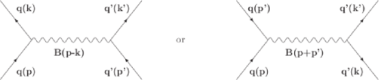
Figure 8: Generic scattering process.

where ${\bf{q}}$, ${\bf{q^{\prime}}}$ and ${\bf{\bar{q}}}$, ${\bf{\bar{q^{\prime}}}}$ are quarks and antiquarks, respectively, and $B_{\mu}$ is some vector boson.

With a Lagrangian of the form ${\cal{L}}={\bar{q}}\gamma^{\mu}qB_{\mu}$, where $B_{\mu}$ is the (generic) vector boson, and the amplitudes corresponding to the diagrams in Fig. 8 are

$$M_{1}\sim\bar{u_{s}}(k)\gamma^{\mu}u_{r}(p){\cal{P}}_{\mu\rho}(p-k)\bar{u_{s}^{\prime}}(k^{\prime})\gamma^{\rho}u_{r}^{\prime}({p^{\prime}}),$$

$$M_{2}\sim\bar{v_{r}^{\prime}}({p^{\prime}})\gamma^{\mu}u_{r}(p){\cal{P}}_{\mu\rho}(p+p^{\prime})\bar{u_{s}^{\prime}}(k^{\prime})\gamma^{\rho}v_{s}(k)$$

where the $u$:s and $v$:s are spinors, $s,r,s^{\prime},r^{\prime}$ are spins, and ${\cal{P}}_{\mu\rho}$ are the boson propagators. The corresponding cross sections are

$$d\sigma=\frac{1}{v_{rel}(2\pi)^{3}}{\frac{|M_{j}|^{2}}{2p_{0}2p^{\prime}_{0}}}\partial^{4}(p+p^{\prime}-k-k^{\prime})\frac{d^{3}kd^{3}k^{\prime}}{2k_{0}2k^{\prime}_{0}}$$ (123)

where $M_{j}$ are the transition amplitudes, $j=1,2$.

For particles in a Lorentz frame, moving collinearly (e.g. the lab system or the Center of Mass system). In such a frame $v_{rel}$ is given by

$$v_{rel}=\frac{{\sqrt{(pp^{\prime})^{2}-m^{2}m^{{}^{\prime}2}}}}{p_{0}p^{\prime}_{0}}$$ (124)

where $m$ = $m_{q}$ and $m^{\prime}$ = $m_{q^{\prime}}$.

The diagrams in Fig. 8 encompass electromagnetic, weak and strong interactions. We are mainly interested in the strong interaction diagrams, but the question is the form of the gluon propagators, since unlike the electromagnetic and weak interactions that can be handled pertubatively, in strong interaction all orders may be of comparable magnitude (i.e. the contributions from the lowest order diagrams are no longer overwhelmingly dominating).

0.32 The cross sections

In order to calculate the cross sections for the prosesses in Fig. 8, we initially use the standard Lagrangian

$${\cal{L}}=\sum_{j=1}^{n_{f}}\bar{q_{j}}(i{\displaystyle{\not}D-m_{j})q_{j}-\frac{1}{4}G_{\mu\nu}G^{\mu\nu}}$$ (125)

where where $n_{f}$ is the number of families, $q_{j}$ is the quark (Dirac) field,

$${\displaystyle{\not}D=(\partial_{\mu}-igA_{\mu})\gamma^{\mu}},$$

$A_{\mu}$ is the gluon field and $G_{\mu\nu}G^{\mu\nu}$ the gluon field strength; and the quark mass parameter $m_{j}$ depends on the renormalization scheme and the scale parameter.

We follow the usual procedures with averaging over initial spins and summing the final spins,

$$\frac{1}{4}\sum_{s,r,s^{\prime},r^{\prime}}|M_{1}|^{2}\sim\frac{1}{4}\sum_{s,r,s^{\prime},r^{\prime}}|\bar{u}_{s}(k)\gamma^{\mu}u_{r}(p){\cal{P}}_{\mu\rho}(p-k)\bar{u}_{s}^{\prime}(k^{\prime})\gamma^{\rho}u_{r}^{\prime}({p^{\prime}})|^{2}=$$

$$=\frac{1}{4}Tr[(\frac{\displaystyle{\not}k+m}{2m})\gamma^{\mu}(\frac{\displaystyle{\not}p+m}{2m})\gamma^{\eta}]$$

$$Tr[(\frac{\displaystyle{\not}k^{\prime}+m^{\prime}}{2m^{\prime}})\gamma^{\rho}(\frac{\displaystyle{\not}{p^{\prime}}+m^{\prime}}{2m^{\prime}})\gamma^{\phi}]{\cal{P}}_{\mu\rho}(p-k){\cal{P}}_{\eta\phi}^{\dagger}(p-k)=$$

$$=\frac{1}{4}\frac{{\cal{P}}_{\mu\rho}(p-k){\cal{P}}_{\eta\phi}^{\dagger}(p-k)}{m^{2}m^{\prime 2}}[k^{\mu}p^{\eta}+k^{\eta}p^{\mu}+g^{\mu\eta}(m^{2}-kp)]$$

$$[k^{\prime\rho}p^{\prime\phi}+k^{\prime\phi}{p^{\prime}}^{\rho}+g^{\rho\phi}(m^{\prime 2}-k^{\prime}{p^{\prime}})]$$ (126)

and

$$\frac{1}{4}\sum_{s,r,s^{\prime},r^{\prime}}|M_{2}|^{2}\sim$$ (127)

$$\sim\frac{1}{4}\frac{{\cal{P}}_{\mu\rho}(p+p^{\prime}){\cal{P}}_{\eta\phi}^{\dagger}(p+p^{\prime})}{m^{2}m^{\prime^{\prime}2}}[{p^{\prime}}^{\mu}p^{\phi}+{p^{\prime}}^{\phi}p^{\mu}-g^{\mu\phi}(pp^{\prime}+m^{2})]$$

$$[k^{\prime\rho}k^{\eta}+k^{\prime\eta}k^{\rho}+g^{\rho\eta}(kk^{\prime}+{m^{\prime}}_{q}^{2})],$$

with the corresponding cross sections

$$d\sigma_{1}=\frac{1}{4v_{rel}(2\pi)^{3}}{\frac{|M_{1}|^{2}}{2p_{0}2p^{\prime}_{0}}}\partial^{4}(p+p^{\prime}-k-k^{\prime})\frac{d^{3}kd^{3}k^{\prime}}{2k_{0}2k^{\prime}_{0}}=$$

$$=\frac{1}{4v_{rel}(2\pi)^{3}}{\cal{P}}_{\mu\rho}(p-k){\cal{P}}_{\eta\phi}^{\dagger}(p-k)\frac{[k^{\mu}p^{\eta}+k^{\eta}p^{\mu}+g^{\mu\eta}(m^{2}-kp)]}{m^{2}m^{\prime 2}}\otimes$$

$$\otimes{\frac{[k^{\prime\rho}p^{\prime\phi}+k^{\prime\phi}{p^{\prime}}^{\rho}+g^{\rho\phi}(m^{\prime 2}-k^{\prime}{p^{\prime}})]}{2p_{0}2p^{\prime}_{0}}}\partial^{4}(p+p^{\prime}-k-k^{\prime})\frac{d^{3}kd^{3}k^{\prime}}{2k_{0}2k^{\prime}_{0}}$$ (128)

and

$$d\sigma_{2}=\frac{1}{4v_{rel}(2\pi)^{3}}{\frac{|M_{2}|^{2}}{2p_{0}2p^{\prime}_{0}}}\partial^{4}(p+p^{\prime}-k-k^{\prime})\frac{d^{3}kd^{3}k^{\prime}}{2k_{0}2k^{\prime}_{0}}=$$

$$=\frac{1}{4v_{rel}(2\pi)^{3}}{\cal{P}}_{\mu\rho}(p+{p^{\prime}}){\cal{P}}_{\eta\phi}^{\dagger}(p+{p^{\prime}})\frac{[{p^{\prime}}^{\mu}p^{\phi}+{p^{\prime}}^{\phi}p^{\mu}-g^{\mu\phi}(p{p^{\prime}}+m^{2})]}{m^{2}m^{\prime 2}}\otimes$$

$$\otimes{\frac{[k^{\prime\rho}k^{\eta}+k^{\prime\eta}k^{\rho}+g^{\rho\eta}(kk^{\prime}+{m^{\prime}}_{q}^{2})]}{2p_{0}2p^{\prime}_{0}}}\partial^{4}(p+p^{\prime}-k-k^{\prime})\frac{d^{3}kd^{3}k^{\prime}}{2k_{0}2k^{\prime}_{0}}$$ (129)

In calculating the first process, we go to the lab system, where ${\bf{p^{\prime}}}$ = 0, and

$$pp^{\prime}=(p_{0},{\bf{p}})(p^{\prime}_{0},{\bf{0}})=p_{0}p^{\prime}_{0},$$

so

$$v_{rel}=\frac{|{\bf{p}}|}{p_{0}},$$

and the cross section reads

$$d\sigma_{1}=\frac{p_{0}}{4(2\pi)^{3}|{\bf{p}}|}{\frac{|M_{1}|^{2}}{2p_{0}2p^{\prime}_{0}}}\partial^{4}(p+p^{\prime}-k-k^{\prime})\frac{d^{3}kd^{3}k^{\prime}}{2k_{0}2k^{\prime}_{0}}=$$

$$=\frac{p_{0}}{4(2\pi)^{3}|{\bf{p}}|}{\cal{P}}_{\mu\rho}(p-k){\cal{P}}_{\eta\phi}^{\dagger}(p-k)\frac{[k^{\mu}p^{\eta}+k^{\eta}p^{\mu}+g^{\mu\eta}(m^{2}-kp)]}{m^{2}m^{\prime 2}}\otimes$$

$$\otimes{\frac{[k^{\prime\rho}p^{\prime\phi}+k^{\prime\phi}{p^{\prime}}^{\rho}+g^{\rho\phi}(m^{\prime 2}-k^{\prime}{p^{\prime}})]}{2p_{0}2p^{\prime}_{0}}}\partial^{4}(p+p^{\prime}-k-k^{\prime})\frac{d^{3}kd^{3}k^{\prime}}{2k_{0}2k^{\prime}_{0}}$$ (130)

For the second process, we go to the center of mass system, i.e. ${\bf{p^{\prime}}}$ = -${\bf{p}}$, so

$$v_{rel}=|{\bf{p}}|\frac{(p_{0}+p^{\prime}_{0})}{p_{0}p^{\prime}_{0}},$$

and

$$d\sigma_{2}=\frac{p_{0}p^{\prime}_{0}}{{4|{\bf{p}}|}(p_{0}+p^{\prime}_{0})(2\pi)^{3}}{\frac{|M_{2}|^{2}}{2p_{0}2p^{\prime}_{0}}}\partial^{4}(p+p^{\prime}-k-k^{\prime})\frac{d^{3}kd^{3}k^{\prime}}{2k_{0}2k^{\prime}_{0}}=$$

$$=\frac{p_{0}p^{\prime}_{0}}{4|{\bf{p}}|(p_{0}+p^{\prime}_{0})(2\pi)^{3}}{\cal{P}}_{\mu\rho}(p+{p^{\prime}}){\cal{P}}_{\eta\phi}^{\dagger}(p+{p^{\prime}})$$

$$\frac{[{p^{\prime}}^{\mu}p^{\phi}+{p^{\prime}}^{\phi}p^{\mu}-g^{\mu\phi}(p{p^{\prime}}+m^{2})]}{m^{2}m^{\prime 2}}\otimes$$

$$\otimes{\frac{[k^{\prime\rho}k^{\eta}+k^{\prime\eta}k^{\rho}+g^{\rho\eta}(kk^{\prime}+{m^{\prime}}_{q}^{2})]}{2p_{0}2p^{\prime}_{0}}}\partial^{4}(p+p^{\prime}-k-k^{\prime})\frac{d^{3}kd^{3}k^{\prime}}{2k_{0}2k^{\prime}_{0}}$$ (131)

0.33 Gluon propagators

There are several methods to obtain the gluon propagator by using non-perturbative methods, like in lattice field theory or the Dyson-Schwinger equations (an infinite system of non-linear coupled integral equations relating the different Green functions of a quantum field theory). There are many different solutions for both methods, and in many cases it is useful to introduce a dynamical gluon mass corn .

In a general covariant gauge, the gluon propagator can be expressed burden

$$g\texttwosuperior D_{\mu\nu}(Q)=(\delta_{\mu\nu}-Q_{\mu}Q_{\nu}/Q^{2})\Delta(Q^{2})+g^{2}\xi Q_{\mu}Q_{\nu}/Q^{2}$$ (132)

where $\xi$ is a gauge fixing parameter.

We merely want to know how the cross sections depend on the quark masses. For $d\sigma_{2}$ we go to the CM system and represent the gluon propagator by a a generic expression, neglecting the subtleties of transversal and longitudinal terms, $P_{\alpha\beta}\sim(\delta_{\alpha\beta}-Q_{\alpha}Q_{\beta}/Q\texttwosuperior)$. This gives, for $Q=p+p^{\prime}=k+k^{\prime}$,

$$d\sigma_{2}\sim\frac{p_{0}p^{\prime}_{0}}{4|{\bf{p}}|(p_{0}+p^{\prime}_{0})(2\pi)^{3}}(\delta_{\mu\rho}-\frac{Q_{\mu}Q_{\rho}}{Q^{2}})(\delta_{\eta\phi}-\frac{Q_{\eta}Q_{\phi}}{Q^{2}})$$

$$\frac{[{p^{\prime}}^{\mu}p^{\phi}+{p^{\prime}}^{\phi}p^{\mu}-g^{\mu\phi}(p{p^{\prime}}+m^{2})]}{m^{2}m^{{}^{\prime}2}}\otimes$$

$$\otimes{\frac{[k^{\prime\rho}k^{\eta}+k^{\prime\eta}k^{\rho}+g^{\rho\eta}(kk^{\prime}+{m^{\prime}}^{2})]}{2p_{0}2p^{\prime}_{0}}}\partial^{4}(p+p^{\prime}-k-k^{\prime})\frac{d^{3}kd^{3}k^{\prime}}{2k_{0}2k^{\prime}_{0}}=$$

$$=\frac{2[(pk)(p^{\prime}k^{\prime})+(pk^{\prime})(p^{\prime}k)]+Q^{2}(m^{\prime 2}-m^{2})-Q^{4}}{64|{\bf{p}}|(p_{0}+p^{\prime}_{0})(2\pi)^{3}m^{2}m^{\prime 2}}$$

$$\partial^{4}(p+p^{\prime}-k-k^{\prime})\frac{d^{3}kd^{3}k^{\prime}}{k_{0}k^{\prime}_{0}}$$ (133)

Likewise for the first process in Fig. 8 (in lab system). In the limit of very heavy quark masses, it is perhaps more realistic to use the static HQET Lagrangian below.

This is just an attempt to get a grip on the form of these (very basic) cross sections, well aware of the fact that QCD is very different at different energy scales, and that the form of the gluon propagators therefore need a careful consideration.

In fact, QCD is really a multi-scale theory:

$$m\ll\Lambda\ll m$$

$$m=m_{u},m_{d},m_{s}$$

$$m=m_{c},m_{b},m_{t},...$$

$$\Lambda\sim 700MeV$$

There are two more scales: for the ultraviolet cutoff $(\pi/a)$ and the infrared cutoff (${L^{-1}}$). In principle we have ${{L^{-1}}}\ll m\ll\Lambda\ll m_{b}\ll\pi/a$, but in practice ${L^{-1}}\ll m\ll\Lambda\ll m_{b}\sim\pi/a$.

A multi-scale problem can be dealt with by introducing some scale-separating scheme (like an effective field theory), this is precisely what is done in lattice QCD. An effective field theory separates short-distance effects from long-distance effects by introducing a separation scale to place a boundary between “long” and “short”, and also introducing new fields that to describe the long-distance part, and then equating the effective theory and the underlying theory, i.e. $L_{underlying}=L_{effective}$.

The electroweak effective Hamiltonian is an example of this. The underlying theory is the Standard Model, and the effective Hamiltonian is a theory of photons, gluons, and the five lighter quarks.

Another example is the non-relativistic effective theory for heavy quarks, like the heavy-quark effective theory (HQET) and non-relativistic QCD. Heavy-quark fields in underlying theory has four components; in effective theory two components. These can be derived to all orders in QED and QCD perturbation theory.

0.34 Heavy Quark Effective Theory

The Heavy Quark Effective Theory, HQET, is an effective theory that is obtained from QCD by performing a $1/m$ expansion, where $m$ is the heavy quark mass. In the infinite mass limit the heavy quark acts like a static colour source. The momentum $p_{q}$ of the heavy quark scales with the mass, therefore one uses the quark velocity $v$ as the kinematic parameter. Taking the heavy quark momentum to be $p_{q}=mv+p^{\prime}=m(v+p^{\prime}/m)$, where $p^{\prime}$ is the part of the momentum that does not scale with the mass, we can express the heavy quark field (in full QCD) as

$$Q(x)=e^{-imvx}[1+(\frac{1}{2m+ivD})i\displaystyle{\not}{D}_{\perp}]q_{v}$$

$$=e^{-imvx}[1+\frac{1}{2m}\displaystyle{\not}{D}_{\perp}+(\frac{1}{2m})^{2}(-iDv)\displaystyle{\not}{D}_{\perp}+...]q_{v}$$ (134)

and the Lagrangian

$${\cal{L}}=\bar{q}_{v}(ivD)q_{v}+\bar{q}_{v}i\displaystyle{\not}{D}_{\perp}(\frac{1}{2m+ivD})i\displaystyle{\not}{D}_{\perp}q_{v}=$$ (135)

$$=\bar{q}_{v}(ivD)q_{v}+\frac{1}{2m}\bar{q}_{v}(i\displaystyle{\not}{D}_{\perp})^{2}iq_{v}+(\frac{1}{2m})^{2}\bar{q}_{v}(i\displaystyle{\not}{D}_{\perp})(-ivD)(i\displaystyle{\not}{D}_{\perp})q_{v}+..$$

where $D$ is the covariant derivative of QCD, and $1/m$ is the mass of the heavy quark field $Q$ in full QCD, and $q_{v}$ is the static heavy quark moving with velocity $v$, corresponding to the upper components of the full field, since

$P_{(+)}q_{v}=q_{v}$, $P_{(-)}q_{v}=0$, $P_{(\pm)}=(\displaystyle{\not}{v}\pm 1)/2$. The leading terms of these expansions define the static limit with the static Lagrangian

$${\cal{L}}_{stat}=\bar{q}_{v}(ivD)q_{v}$$ (136)

that describes the heavy degrees of freedom.

In the case when bottom and charm are perceived as be heavy, the static Lagrangian for both quarks is written

$${\cal{L}}_{stat}=\bar{b}_{v_{b}}(ivD)b_{v_{b}}+\bar{c}_{v_{c}}(ivD)c_{v_{c}}$$ (137)

where $b_{v_{b}}$ and $c_{v_{c}}$ are the bottom and charm quarks moving with velocities $v_{c}$ and $v_{b}$, respectively. Notice that the quark masses do not appear in the Lagrangian, which means that the Lagrangian has a heavy flavour symmetry which allows rotations of the $b$- and $c$-fields into each other.

Both spin directions of the heavy quark couple in the same way to the gluons as well, so the Lagrangian has a symmetry under rotations of the heavy quark spin, so all the heavy hadron states that move with velocity $v$ fall into spin-symmetry doublets in the infinite mass limit.

0.35 How to proceed

We should discuss which processes should be considered, i.e. what scattering processes (involving heavy fermions) would be characteristic within this scenario. We should moreover discuss what gluon propagators we should use, and also consider the electroweak contribution to the cross sections.

PRESENTATION OF
VIRTUAL INSTITUTE OF ASTROPARTICLE PHYSICS
AND
BLED 2008 WORKSHOP VIDEO CONFERENCE

M.Yu. Khlopov^1,2,3 Scientific-Educational Complex — Virtual Institute of Astroparticle Physics

0.36 Introduction

Studies in astroparticle physics link astrophysics, cosmology and particle physics and involve hundreds of scientific groups linked by regional networks (like ASPERA/ApPEC mk2viaaspera ) and national centers. The exciting progress in precision cosmology, in gravitational wave astronomy, in underground, cosmic-ray and accelerator experiments promise large amount of a new information and discoveries in coming years. Theoretical analysis of these results will have impact on the fundamental knowledge on the structure of microworld and Universe and on the basic, still unknown, physical laws of Nature (see e.g. mk2viabook for review).

It is clear that the effectiveness of the work depends strongly on the number of groups involved in this activity, on the information exchange rate and on the overall coordination. An international forum, be it virtual, which can join all the groups and coordinate their efforts would give a boost to this cooperation. Particularly this is important for isolated scientific groups and scientists from small countries which can contribute a lot to this work being a part of the large international collaboration. A possibility of education on distance, involving young people from all over the world, is another important aspect of this activity.

A good example of such kind of structure is an International Virtual Observatory mk2viaIVOA , created in 2002. It has demonstrated the work effectiveness and fruitful cooperation of many organizations all over the world. Problems of Virtual Laboratories were discussed in mk2viaHut:2007ke .

In the proposal mk2viaKhlopov:2008vd it was suggested to organize a Virtual Institute of Astroparticle Physics (VIA), which can play the role of such unifying and coordinating structure for astroparticle physics. Starting from the January of 2008 the activity of the Institute takes place on its website mk2viaVIA in a form of regular weekly video conferences with VIA lectures, covering all the theoretical and experimental activities in astroparticle physics and related topics. The library of records of these lectures and their presentations is now accomplished by multi-lingual forum. Here the general structure of VIA complex and the format of its video conferences are stipulated to clarify the way in which VIA discussion of puzzles of dark matter searches took place in the framework of Bled Workshop.

0.37 The structure of VIA complex

The structure of VIA complex is illustrated on Fig. 9.

Figure 9: The home page of VIA site

The home page, presented on this figure, contains the information on VIA activity and menu, linking to directories (along the upper line from left to right): with general information on VIA (What is VIA), to Forum, to VIA virtual lecture hall and meeting rooms (Rooms), to the library of records and presentations of VIA lectures and courses (Previous) and to contact information (Contacts). The announcement of the next Virtual meeting, the calender with the program of future lectures and courses together with the links to VIA news and posters as well as the instructions How to use VIA are also present on the home page. The VIA forum, now being ready to operate, is intended to cover the topics: beyond the standard model, astroparticle physics, cosmology, gravitational wave experiments, astrophysics, neutrinos. Presently activated in English, French and Russian with trivial extension to other languages, the Forum represents a first step on the way to multi-lingual character of VIA complex and its activity.

0.38 VIA lectures and virtual meetings

First tests of VIA system, described in mk2viaKhlopov:2008vd , involved various systems of video conferencing. They included skype, VRVS, EVO, WEBEX, marratech and adobe Connect. In the result of these tests the adobe Connect system was chosen and properly acquired. Its advantages are: relatively easy use for participants, a possibility to make presentation in a video contact between presenter and audience, a possibility to make high quality records and edit them, removing from records occasional and rather rare disturbances of sound or connection, to use a whiteboard facility for discussions, the option to open desktop and to work online with texts in any format. The regular form of VIA meetings assumes that their time and Virtual room are announced in advance. Since the access to the Virtual room is strictly controlled by administration, the invited participants should enter the Room as Guests, typing their names, and their entrance and successive ability to use video and audio system is authorized by the Host of the meeting. The format of VIA lectures and discussions is shown on Fig. 10.

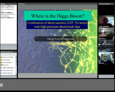
Figure 10: Video conference with lecture by John Ellis, which he gave from his office in CERN, Switzerland, became a part of the program of XIII Summer Institute on Astroparticle physics in Gran Sasso, Italy

The ppt file of presentation is uploaded in the system in advance and then demonstrated in the central window. Video images of presenter and participants appear in the right window, while in the lower left window the list of all the attendees is given. To protect the quality of sound and record, the participants are required to switch out their audio system during presentation and to use upper left Chat window for immediate comments and urgent questions. The Chat window can be also used by participants, having no microphone, for questions and comments during Discussion. In the end of presentation the central window can be used for a whiteboard utility as well as the whole structure of windows can be changed, e.g. by making full screen the window with the images of participants of discussion.

0.39 VIA Discussion Session at Bled Workshop

VIA discussion session took place in the framework of Bled Workshop on 24 July. It contained presentations: by N.S. Mankoč Borštnik about dark matter candidates following from her approach, unifying spins and charges, by G. Bregar about the possibility to explain the results of dark matter searches by some of these candidates, M. Yu. Khlopov about the composite dark matter scenario and by A.Mayorov and E. Soldatov about the application of this scenario to solution of the controversy between the results of DAMA and CDMS experiments. The content of these presentations can be found in the contributions mk2viaBled . To clarify the possibilities to explain the positive results of DAMA/NaI and DAMA/Libra experiments without contradiction with strong constraints, which follow from the results of CDMS experiment, J.Filippini (Berkeley,USA) from CDMS collaboration took part in Discussion (Fig. 11). His arguments can be found in the Discussion section of this volume.

Figure 11: Bled Conference Discussion Bled-Moscow-Berkeley

In spite of technical problem for some participants the main root of virtual meeting, which was organized in Bled,Slovenia and involved J.Filippini in Berkeley, USA and A.Mayorov, E.Soldatov and other participants from Moscow, Russia was stable during all the 3 hours of the video conference.

0.40 Conclusions

The exciting experiment of VIA Discussion at Bled Workshop, the three days of permanent online transmissions and distant participation in the Gran Sasso Summer Institute on Astroparticle physics, the VIA interactive form of Seminars in Moscow and in Pisa with participation and presentation on distance, the stable regular weekly video conferences with VIA lectures and the solid library of their records and presentations, creation of multi-lingual VIA Internet forum, regular basic courses and individual work on distance with students of MEPhI prove that the Scientific-Educational complex of Virtual Institute of Astroparticle physics can provide regular communications between different groups and scientists, working in different scientific fields and parts of the world, get the first-hand information on the newest scientific results, as well as to support various educational programs on distance. This activity would easily allow finding mutual interest and organizing task forces for different scientific topics of astroparticle physics. It can help in the elaboration of strategy of experimental particle, nuclear, astrophysical and cosmological studies as well as in proper analysis of experimental data. It can provide young talented people from all over the world to get the highest level education, come in direct interactive contact with the world known scientists and to find their place in the fundamental research. To conclude the VIA complex is in operation and ready for a wide use and applications.

Acknowledgements

The initial step of creation of VIA was supported by ASPERA. I am grateful to S.Katsanevas for permanent stimulating support, to P.Binetruy, J.Ellis, F.Fidecaro, M.Pohl for help in development of the project, to K.Belotsky and K.Shibaev for assistance in educational VIA program and to A.Mayorov and E.Soldatov for cooperation in its applications, to Z.Berezhiani and all Organizers of XIII Summer School on Astroparticle Physics in Gran Sasso for cooperation in the use of VIA for online distant participation and to D.Rouable for help in technical realization and support of VIA complex. I express my gratitude to N.S. Mankoč Borštnik, G.Bregar, D. Lukman and all Organizers of Bled Workshop for cooperation in the exciting experiment of VIA Discussion Session at Bled.

References

- (1) R. Bernabei at al, Int.J.Mod.Phys. D13 (2004) 2127-2160, astro-ph/0501412, astro-ph/0804.2738v1.
- (2) Z. Ahmed et al., pre-print, astro-ph/0802.3530.
- (3) C. Amsler et al., Physics Letters B667, 1 (2008), available on the PDG WWW pages (http://pdg.lbl.gov/)
- (4) S. Dodelson, Modern Cosmology, Academic Press Elsevier 2003.
- (5) A. Borštnik Bračič, N.S. Mankoč Borštnik, Phys Rev. D 74 (2006) 073013-16.
- (6) N.S. Mankoč Borštnik, Phys. Lett. B 292 (1992) 25-29,
- (7) N.S. Mankoč Borštnik, “Spinor and vector representations in four dimensional Grassmann space”, J. Math. Phys. 34 (1993) 3731-3745, Modern Phys. Lett. A 10 (1995) 587-595,
- (8) N. S. Mankoč Borštnik, Int. J. Theor. Phys. 40 (2001) 315-337,
- (9) N. S. Mankoč Borštnik, hep-ph/0711.4681, 94-113.
- (10) G. Bregar, M. Breskvar, D. Lukman, N.S. Mankoč Borštnik, New J. of Phys. 10 (2008) 093002.
- (11) N.S. Mankoč Borštnik, H.B. Nielsen, J. of Math. Phys. 43 (2002), (5782-5803), J. of Math. Phys. 44 (2003) 4817-4827.
- (12) G. Bregar, N.S. Mankoč Borštnik, hep-ph/0711.4681, 189-194.
- (13) N.S. Mankoč Borštnik, H.B. Nielsen, Proceedings to the International Workshop ”What Comes Beyond the Standard Model”, 13 -23 of Ju;y, 2002, VolumeII, Ed. Norma Mankoč Borštnik, Holger Bech Nielsen, Colin Froggatt, Dragan Lukman, DMFA Založništvo, Ljubljana December 2002, hep-ph/0301029.
- (14) W. Greiner, E. Stein, S. Schramm, Quantum Chromodynamics, Springer 2002, p. 215.
- (15) G. Bregar, M. Khlopov, N.S. Mankoč Borštnik, work in progress.
- (16) We thank cordialy R. Bernabei (in particular) and J. Filippini for very informative discussions by web mail and in private communication.
- (17) Maxim Yu. Khlopov, JETP Lett. 83, 1 (2006) [Pisma Zh. Eksp. Teor. Fiz. 83, 3 (2006)]; arXiv:astro-ph/0511796, pre-print, astro-ph/0806.3581.

References

- (1) S. Weinberg: “Feynman Rules for Any Spin”, Phys. Rev. 133B (1964) 1318; “Feynman Rules for Any Spin II. Massless Particles”, Phys. Rev. 134B (1964) 882; R. H. Tucker and C. L. Hammer: “New Quantum Electrodynamics for Vector Mesons”, Phys. Rev. D3 (1971) 2448.
- (2) V. Dvoeglazov: “- Component Model and its Connection with Other Field Theories”, Rev. Mex. Fis. Suppl. 40 (1994) 352; “Quantized Fields”, Int. J. Theor. Phys. 37 (1998) 1915; “Generalizations of the Dirac Equation and the Modified Bargmann-Wigner Formalism”, Hadronic J. 26 (2003) 299.
- (3) D. V. Ahluwalia and M. Sawicki: “Front Form Spinors in the Weinberg-Soper Formalism and Generalized Melosh Transformations for Any Spin”, Phys. Rev. D47 (1993) 5161.
- (4) L. D. Landau and E. M. Lifshitz: The Classical Theory of Fields. Pergamon Press, Oxford, 1975.
- (5) L. H. Ryder: Quantum Field Theory. Cambridge University Press, Cambridge, 1985.
- (6) E. P. Wigner: “On Unitary Representations of the Inhomogeneous Lorentz Group”, Ann. Math. 40 (1939) 149.
- (7) In Review of Particle Physics. Phys. Lett. B592 (2004), 31.

References

- (1) H. Snyder: Phys. Rev. 71, 38 (1947); ibid. 72, 68 (1947).
- (2) S. Doplicher et al.: Phys. Lett. B331, 39 (1994); S. Majid and H. Ruegg: Phys. Lett. B334, 348 (1994); J. Lukierski, H. Ruegg and W. J. Zakrzewski: Ann. Phys. 243, 90 (1995); N. Seiberg and E. Witten: JHEP 9909, 032 (1999), hep-th/9908142; I. F. Riad and M. M. Sheikh-Jabbari: JHEP 08, 045 (2000), hep-th/0008132; M. M. Sheikh-Jabbari: Phys. Rev. Lett. 84, 5265 (2000), hep-th/0001167; J. Madore et al.: Eur. Phys. J. C16, 161 (2000); S. I. Kruglov: Ann. Fond. Broglie 27, 343 (2002).
- (3) F. Dyson: Am. J. Phys. 58, 209 (1990); S. Tanimura: Ann. Phys. 220, 229 (1992); see also many subsequent comments on these works.
- (4) A. E. Chubykalo and R. Smirnov-Rueda: Mod. Phys. Lett A12, 1 (1997); A. E. Chubykalo and S. Vlayev: Int. J. Mod. Phys. A14, 3789 (1999); A. E. Chubykalo, R. A. Flores and J. A. Pérez: in Proc. of the Internatinal Workshop “Lorentz Group, CPT and Neutrinos”, Zacatecas, México, June 1999. Eds. A. E. Chubykalo, V. V. Dvoeglazov et al. World Scientific, 2000, 384-396; A. E. Chubykalo and R. A. Flores: Hadronic J. 25, 159 (2002).
- (5) K. R. Brownstein: Am. J. Phys. 67, 639 (1999); J. D. Jackson: hep-ph/0203076, L. Škovrlj and T. Ivezić: hep-ph/0203116; V. Dvoeglazov, Spacetime and Substance: 3, 125 (2002).
- (6) V. Y. Arnold, Mathematical Methods of Classical Mechanics. (Springer-Verlag, 1989), p. 258; L. Schwartz, Analyse Mathématique. Vol. 1 (HERMANN, Paris, 1967).
- (7) L. D. Landau and E. M. Lifshitz: The Classical Theory of Fields. 4th revised English ed. Translated from the 6th Russian edition. Pergamon Press, 1979. 402p., §63.
- (8) M. Jacob y G. C. Wick: Ann. Phys. 7, 404 (1959); H. M. Ruck y W. Greiner: J. Phys. G: Nucl. Phys. 3, 657 (1977).
- (9) A. Kempf, G. Mangano and R. B. Mann: Phys. Rev. D52 , 1108 (1995); G. Amelino-Camelia: Nature 408, 661 (2000); gr-qc/0012051; hep-th/0012238; gr-qc/0106004; J. Kowalski-Glikman: hep-th/0102098; G. Amelino-Camelia and M. Arzano: hep-th/0105120; N. R. Bruno, G. Amelino-Camelia and J. Kowalski-Glikman: hep-th/0107039.
- (10) V. V. Dvoeglazov: Rev. Mex. Fis. Supl. 49, 99 (2003) (Proceedings of the DGFM-SMF School, Huatulco, 2000).
- (11) R. A. Berg: Nuovo Cimento 42A, 148 (1966); V. V. Dvoeglazov: ibid. A108, 1467 (1995).
- (12) A. D. Donkov et al., Bull.Russ.Acad.Sci.Phys. 46, 126 (1982); V. G. Kadyshevsky et al., Nuovo Cim. A87, 373 (1985).

References

- (1) M.Yu. Khlopov Cosmoparticle physics (World Scientific, Singapore, 1999).
- (2) M.Yu. Khlopov in Cosmion-94, Eds. M.Yu.Khlopov et al. (Editions frontieres, 1996) P. 67; M. Y. Khlopov in hep-ph/0612250 , p 51.
- (3) M. Y. Khlopov in arXiv:0711.4681, p. 114; M. Y. Khlopov and N. S. Mankoc-Borstnik, ibid, p. 195.
- (4) M.Yu. Khlopov, JETP Lett. 83, 1 (2006).
- (5) K. Belotsky et al, arXiv:astro-ph/0602261. K. Belotsky et al, Gravitation and Cosmology 12, 1 (2006); K. Belotsky et al, arXiv:0806.1067 [astro-ph].
- (6) M. Y. Khlopov, arXiv:astro-ph/0607048.
- (7) K.M.Belotsky et al, Gravitation and Cosmology Supplement 6, 140 (2000) K.M.Belotsky et al, Phys.Atom.Nucl. 71, 147 (2008); K.M. Belotsky et al, Gravitation and Cosmology 11, 27 (2005); K.M.Belotsky et al, Gravitation and Cosmology 11, 16 (2005) and references therein.
- (8) K.M.Belotsky et al, Gravitation and Cosmology 11, 3 (2005)
- (9) M. Maltoni et al, Phys. Lett. B 476, 107 (2000); V.A. Ilyin et al, Phys. Lett. B 503, 126 (2001); V.A. Novikov et al, Phys. Lett. B 529, 111 (2002); JETP Lett. 76, 119 (2002).
- (10) S. L. Glashow, arXiv:hep-ph/0504287.
- (11) D. Fargion and M. Khlopov, arXiv:hep-ph/0507087.
- (12) C. A. Stephan, arXiv:hep-th/0509213.
- (13) A. Connes Noncommutative Geometry (Academic Press, London and San Diego, 1994).
- (14) D. Fargion et al, Class. Quantum Grav. 23, 7305 (2006); M. Y. Khlopov and C. A. Stephan, arXiv:astro-ph/0603187.
- (15) M. Y. Khlopov and C. Kouvaris, Phys. Rev. D 77, 065002 (2008).
- (16) F. Sannino and K. Tuominen, Phys. Rev. D 71, 051901 (2005); D. K. Hong et al, Phys. Lett. B 597, 89 (2004); D. D. Dietrich et al, Phys. Rev. D 72, 055001 (2005); D. D. Dietrich et al, arXiv:hep-ph/0510217; S. B. Gudnason et al, Phys. Rev. D 73, 115003 (2006); S. B. Gudnason et al, Phys. Rev. D 74, 095008 (2006).
- (17) G.Bregar and N.S. Mankoč Borštnik, This Volume; A. Borštnik Bračič, N.S. Mankoč Borštnik, Phys. Rev. D 74, 073013 (2006); N.S. Mankoč Borštnik, Mod. Phys. Lett. A 10, 587 (1995); N.S. Mankoč Borštnik, Int. J. Theor. Phys. 40, 315 (2001); G. Bregar, M. Breskvar, D. Lukman, N.S. Mankoč Borštnik, New J. of Phys. 10, 093002 (2008).
- (18) M. Y. Khlopov, arXiv:0801.0167 [astro-ph]; M. Y. Khlopov, arXiv:0801.0169 [astro-ph].
- (19) M. Y. Khlopov, arXiv:0806.3581 [astro-ph].
- (20) C. B. Dover et al, Phys. Rev. Lett. 42, 1117 (1979); S. Wolfram, Phys. Lett. B 82, 65 (1979); G. D. Starkman et al, Phys. Rev. D 41, 3594 (1990); D. Javorsek et al, Phys. Rev. Lett. 87, 231804 (2001); S. Mitra, Phys. Rev. D 70, 103517 (2004); G. D. Mack et al, Phys. Rev. D 76, 043523 (2007).
- (21) B. D. Wandelt et al., arXiv:astro-ph/0006344; P. C. McGuire and P. J. Steinhardt, arXiv:astro-ph/0105567; G. Zaharijas and G. R. Farrar, Phys. Rev. D 72, 083502 (2005).
- (22) M. Y. Khlopov and C. Kouvaris, Phys. Rev. D 78, 065040 (2008).
- (23) R. Bernabei et al., Rivista Nuovo Cimento 26, 1 (2003); Int. J. Mod. Phys. D13, 2127 (2004).
- (24) R. Bernabei et al. [DAMA Collaboration], Eur. Phys. J. C 56, 333 (2008).
- (25) R. N. Cahn and S. L. Glashow, Science 213, 607 (1981); M. Pospelov, Phys. Rev. Lett. 98, 231301 (2007); K. Kohri and F. Takayama, Phys. Rev. D 76, 063507 (2007).
- (26) A. G. Mayorov, ”Search for Stable heavy charged particles of dark matter in the experiment PAMELA”, PreDiplom Report, MIFI, Moscow, 2008.
- (27) D. P. Finkbeiner and N. Weiner, Phys. Rev. D 76, 083519 (2007).
- (28) B. J. Teegarden et al, Astrophys. J. 621, 296 (2005).
- (29) D. McCammon et al, Nucl. Instrum. Methods A 370, 266 (1996); D. McCammon et al, Astrophys. J. 576, 188 (2002).
- (30) K. Belotsky et al, arXiv:astro-ph/0606350.
- (31) D. S. Akerib et al. [CDMS Collaboration], Phys. Rev. Lett. 96, 011302 (2006); Z. Ahmed et al. [CDMS Collaboration], arXiv:0802.3530 [astro-ph].
- (32) R. Bernabei et al., Int. J. Mod. Phys. A22, 3155 (2007).
- (33) R. Bernabei et al. [DAMA Collaboration], Nucl. Instrum. Methods A 592, 297 (2008).
- (34) C. L. Chang et al. [CDMS Collaboration], Nucl. Instrum. Methods A 520, 116 (2004); N. Mirabolfathi et al. [CDMS Collaboration], Nucl. Instrum. Methods A 559, 417 (2006).
- (35) F. Petriello and K. M. Zurek, JHEP 0809, 047 (2008); R. Foot, Phys. Rev. D 78, 043529 (2008); J. L. Feng, J. Kumar and L. E. Strigari, arXiv:0806.3746 [hep-ph]; J. L. Feng, J. Kumar, J. Learned and L. E. Strigari, arXiv:0808.4151 [hep-ph]; E. M. Drobyshevski, arXiv:0811.0151 [astro-ph].
- (36) G. B. Gelmini, arXiv:0810.3733 [hep-ph].
- (37) L. D. Landau, E. M. Lifshitz Quantum Mechanics: Non-Relativistic Theory (Fizmatlit, Moscow, 2004).

References

- (1) N. S. Mankoč Borštnik, Phys. Lett. B 292 (1992) 25.
- (2) N. S. Mankoč Borštnik, J. Math. Phys. 34 (1993) 3731.
- (3) N. S. Mankoč Borštnik, Int. J. Theor. Phys. 40 315 (2001).
- (4) N. S. Mankoč Borštnik, Modern Phys. Lett. A 10 (1995) 587.
- (5) A. Borštnik, N. S. Mankoč Borštnik, hep-ph/0401043, hep-ph/0401055, hep-ph/0301029.
- (6) A. Borštnik Bračič, N.S. Mankoč Borštnik, Phys. Rev. D 74 (2006)073013, hep-ph/0512062.
- (7) G. Bregar, M. Breskvar, D. Lukman, N.S. Mankoč Borštnik, hep-ph/0711.4681.
- (8) G. Bregar, M. Breskvar, D. Lukman, N.S. Mankoč Borštnik, New J. of Phys. 10 (2008) 093002, hep-ph/0606159, hep/ph-07082846.
- (9) E. Witten, Nucl. Phys. B 186 (1981) 412; Princeton Technical Rep. PRINT -83-1056, October 1983.
- (10) N. S. Mankoč Borštnik, H. B. Nielsen, Phys. Lett. B 633 (2006) 771-775, hep-th/0311037, hep-th/0509101.
- (11) N. S. Mankoč Borštnik, H. B. Nielsen, Phys. Lett. B 644 (2007)198-202, hep-th/0608006.
- (12) N. S. Mankoč Borštnik, H. B. Nielsen, Phys. Lett. B 10.1016 (2008).
- (13) N. S. Mankoč Borštnik, H. B. Nielsen, D. Lukman, hep-ph/0412208.
- (14) S. Deser, gr-qc/9512022.
- (15) N. S. Mankoč Borštnik, H. B. Nielsen, J. of Math. Phys. 43 (2002) 5782, hep-th/0111257.
- (16) N. S. Mankoč Borštnik, H. B. Nielsen, J. of Math. Phys. 44 (2003) 4817, hep-th/0303224.
- (17) N. S. Mankoč Borštnik, H. B. Nielsen, Phys. Lett. B 633 (2006) 771, hep-th/0311037, hep-th/0509101.
- (18) M. Blagojević, Gravitation and gauge symmetries (I. of Phys. Pub, ISBN 0750307676, 2001).

References

- (1) Borstnik, Norma Mankoc, Holger Bech Nielsen, Colin D. Froggatt, Dragan Lukman (2004), ”Proceedings to the 7th Workshop ’What comes beyond the Standard models’, July 19 – July 31. 2004, Bled, Slovenia”, Bled Workshops in Physics, Volume 5, #2, December.
- (2) Borstnik, Norma Mankoc, Holger Bech Nielsen, Colin D. Froggatt, Dragan Lukman (2005), ”Proceedings to the 8th Workshop ’What comes beyond the Standard models’, July 19 – July 29. 2005, Bled, Slovenia”, Bled Workshops in Physics, Volume 6, #2, December.
- (3) Borstnik, Norma Mankoc, Holger Bech Nielsen, Colin D. Froggatt, Dragan Lukman (2006), ”Proceedings to the 9th Workshop ’What comes beyond the Standard models’, July 19 – July 29. 2006, Bled, Slovenia”, Bled Workshops in Physics, Volume 7, #2, December.
- (4) Borstnik, Norma Mankoc, Holger Bech Nielsen, Colin D. Froggatt, Dragan Lukman (2007), ”Proceedings to the 10th Workshop ’What comes beyond the Standard models’, July 177 – July 27. 2006, Bled, Slovenia”, Bled Workshops in Physics, Volume 8, #2, December.
- (5) Merzbacher, Eugen (1967), Quantum Mechanics (New York: John Wiley and Sons, Inc.).
- (6) Mirman, R. (1995a), Group Theory: An Intuitive Approach (Singapore: World Scientific Publishing Co.).
- (7) Mirman, R. (1995b), Group Theoretical Foundations of Quantum Mechanics (Commack, NY: Nova Science Publishers, Inc.; republished by Backinprint.com).
- (8) Mirman, R. (1995c), Massless Representations of the Poincaré Group, electromagnetism, gravitation, quantum mechanics, geometry (Commack, NY: Nova Science Publishers, Inc.; republished by Backinprint.com).
- (9) Mirman, R. (1999), Point Groups, Space Groups, Crystals, Molecules (Singapore: World Scientific Publishing Co.).
- (10) Mirman, R. (2001a), Quantum Mechanics, Quantum Field Theory: geometry, language, logic (Huntington, NY: Nova Science Publishers, Inc.; republished by Backinprint.com).
- (11) Mirman, R. (2001b), Quantum Field Theory, Conformal Group Theory, Conformal Field Theory: Mathematical and conceptual foundations, physical and geometrical applications (Huntington, NY: Nova Science Publishers, Inc.; republished by Backinprint.com).
- (12) Mirman, R. (2004a), Geometry Decides Gravity, Demanding General Relativity — It Is Thus the Quantum Theory of Gravity, in rm1nmb , p. 84-93.
- (13) Mirman, R. (2004b), Physics Would Be Impossible in Any Dimension But 3+1 — There Could Be Only Empty Universes, in rm1nmb , p. 94-101.
- (14) Mirman, R. (2004c), Conservation of Energy Prohibits Proton Decay, in rm1nmb , p. 102-106.
- (15) Mirman, R. (2005), Are there Interesting Problems That Could Increase Understanding of Physics and Mathematics? in rm1nm2 , p. 72-78.
- (16) Mirman, R. (2006), How Can Group Theory be Generalized so Perhaps Providing Further Information About Our Universe? in rm1nm3 , p. 80-86.
- (17) Mirman, R. (2006), Our Almost Impossible Universe: Why the laws of nature make the existence of humans extraordinarily unlikely (Lincoln, NE: iUniverse, Inc.)
- (18) Mirman, R. (2006), impunv.wordpress.com; impunv.blogspot.com

References

- (1) R. Bernabei at al, Int.J.Mod.Phys. D13 (2004) 2127-2160, astro-ph/0501412, astro-ph/0804.2738v1.
- (2) Z. Ahmed et al., pre-print, astro-ph/0802.3530.
- (3) See references in the N. S. Mankoč Borštnik (with G. Bregar) talk in this proceedings.
- (4) See record and presentation by N. S. Mankoč Borštnik in Previous, Lectures, VIA site http://www.cosmovia.org.
- (5) See references in the M. Khlopov talk (with A.Mayorov and E.Soldatov) in this procedings.
- (6) See the presentation of the Virtual institute of astroparticle physics in this proceedings.
- (7) See record and presentation by M. Yu. Khlopov in Previous, Lectures, VIA site http://www.cosmovia.org.
- (8) Section Beyond the Standard Model, Forum, VIA site http://www.cosmovia.org.

References

- (1) J. M. Cornwall. Phys. Rev. D, 26:1453–1478, 1982.
- (2) C. J. Burden, Phys. Rev. D 59, 037502-1
- (3) M. B. Gay Ducati, W. K. Sauter, arXiv:hep-ph/0607128v2, arXiv:hep-ph/0110162v1
- (4) U. Häbel, R. Könning, H.-G. Reusch, M. Stingl, and S. Wigard. Z. Phys. A, 336:423–433, 1990, U. Häbel, R. Könning, H.-G. Reusch, M. Stingl, and S. Wigard. Z. Phys. A, 336:435–447, 1990.
- (5) Craig D. Roberts and Sebastian M. Schmidt, ANL-PHY-9530-TH-2000, nucl-th/0005064

References

- (1) http://www.aspera-eu.org/
- (2) M.Yu. Khlopov: Cosmoparticle physics, World Scientific, New York -London-Hong Kong - Singapore, 1999
- (3) http://www.ivoa.net
- (4) P. Hut, arXiv:0712.1655 [astro-ph].
- (5) M. Y. Khlopov, arXiv:0801.0376 [astro-ph].
- (6) http://www.cosmovia.org/
- (7) G. Bregar and N.S. Mankoč Borštnik, This Volume; M.Yu.Khlopov, A.Mayorov and E.Soldatov, This Volume
Blejske Delavnice Iz Fizike, Letnik 9, št. 2, ISSN 1580-4992
Bled Workshops in Physics, Vol. 9, No. 2
Zbornik 11. delavnice ‘What Comes Beyond the Standard Models’, Bled, 15. – 25. julij 2008
Proceedings to the 11th workshop ’What Comes Beyond the Standard Models’, Bled, July 15.–25., 2008
Uredili Norma Mankoč Borštnik, Holger Bech Nielsen in Dragan Lukman
Publikacijo sofinancira Javna agencija za raziskovalno dejavnost Republike Slovenije
Brezplačni izvod za udeležence
Tehnični urednik Vladimir Bensa
Založilo: DMFA – založništvo, Jadranska 19, 1000 Ljubljana, Slovenija
Natisnila BIROGRAFIKA BORI v nakladi 150 izvodov
Publikacija DMFA številka 1724