Hybridization of spin and plasma waves in Josephson tunnel junctions with a ferromagnetic layer.

Abstract

We study dynamics of tunnel Josephson junctions with a thin ferromagnetic layer F [superconductor-insulator-ferromagnet-superconductor (SIFS) junctions]. On the basis of derived equations relating the superconducting phase and magnetic moment to each other we analyze collective excitations in the system and find a new mode which is a hybrid of plasma-like and spin waves. The latter are coupled together in a broad range of parameters characterizing the system. Using the solution describing the collective modes we demonstrate that besides the Fiske steps new peaks appear on the I-V characteristics due to oscillations of the magnetic moment $M$ in the ferromagnetic layer. Thus, by measuring the I-V curve of the SIFS junctions, one can extract an information about the spectrum of spin excitations in the ferromagnet F.

Discovery of the Josephson effects in 1962 was an important step in the development of the condensed matter physics Josephson . Josephson has predicted that the dc current of Cooper pairs with a magnitude of order of the qusiparticle current can flow in the absence of the voltage through a thin insulating layer separating two superconductors S. In the presence of a voltage $V$ the supercurrent oscillates in time with the Josephson frequency $\omega_{J}=2eV/\hbar$.

On the basis of equations describing electrodynamics of the Josephson tunnel junction [superconductor-insulator-superconductor (SIS)] many fascinating phenomena were predicted Josephson ; Barone . For example, small perturbations of the phase difference $\varphi$ may propagate in SIS junctions in a form of Josephson “plasma” waves with the spectrum $\omega^{2}=\Omega_{J}^{2}(1+(kl_{J})^{2}).$ Large perturbations exist in a form of solitons carrying the magnetic flux quantum (fluxons or antifluxons). The interaction of the “plasma” waves with oscillating Josephson currents leads to resonances and peculiarities on the I-V characteristics (Fiske steps) Barone .

The Josephson junctions (JJ) based on conventional superconductors are widely used in practice as generators, the most sensitive detectors of magnetic fields and ac radiation in a wide range of the frequency specrtum, etc Barone . Recently, a considerable progress has been achieved in practical applications of the JJs based on high $T_{c}$ superconductors Koshelev .

Replacing the insulating (I) layer by a ferromagnet (F) one obtains SFS junctions that have been under intensive study during the last decade GolubovRMP ; BuzdinRMP ; BVErmp ; Lyuksyutov . New interesting effects like the so-called $\pi-$state (negative critical Josephson current $j_{c}$) or new type of superconducting correlations (odd triplet superconductivity) may arise in JJs of this type BuzdinRMP ; BVErmp ; EschrigR . Although the main attention was paid to the study of the dc Josephson effect, some ac effects in SFS or SmS (m means a magnetic nanoparticle) junctions have been considered, too acJos ; Braude ; Maekawa .

At the same time, all these studies deal with the SFS junctions where effects like those in tunnel JJs are absent. Experimental studies of the SIFS junctions with an insulating layer I have started quite recently (see Weides and references therein). In these tunnel JJs one can observe collective modes and other dynamical phenomena. Note that the effect of superconductivity on the ferromagnetic resonance has been studied experimentally on S/F bilayers ExpDyn . We have no doubts that proper experiments will be performed in the nearest future and theoretical description of dynamical effects in SIFS or SFIFS tunnel junctions is in great demand.

By now, no theory for dynamical effects in SIFS or SFIFS tunnel junctions has been suggested, although one can expect really new effects. One of the basic properties of the JJs is that they are very sensitive to even very small variations of the magnetic field. So, one can easily imagine that dynamics of the spin degrees of freedom leading to variations of the magnetic field should essentially affect electrodynamics of tunnel SIFS junctions. 

In this paper, we develope theory describing dynamical effects in SIFS or SFIFS junctions. We demonstrate that dynamics of the phase difference $\varphi$ and of the magnetization $M$ is described by two coupled equations which determine dynamics of both the spin and orbital degrees of freedom. One of these equations governs the spatial and temporal evolution of the phase $\varphi$, while the other describes the precession of the magnetization $M.$ Using these equations we investigate collective modes in Josephson junctions with F layers and show that these modes are coupled spin and plasma-like Josephson waves.

Although the influence of the superconducting condensate on spin waves in magnetic superconductors was studied by Braude and Sonin Sonin some time ago, the tunnel JJs with a ferromagnetic layer is a more interesting system because besides the spin waves another mode (plasma-like Josephson waves) exists in these systems. It is our main finding that in such systems the both types of the excitation hybridize forming a new collective mode consisting of coupled oscillations of the magnetization and the Josephson current. Moreover, the spin waves can be excited and recorded simply by passing a dc current $j$ through the junctions, and measuring the I-V characteristics of the junction. We demonstrate below that peculiarities on the I-V curve (Fiske steps) bear information about the spectrum of the system, which can be considered as the basis of a new type of spectroscopy of spin excitations in a ferromagnet.

The hybridization of the charge and spin excitations occurs because the contribution to the magnetic moment in the system comes from both orbital electron motion and exchange field. The orbital currents are affected by spins of the ferromagnets and vice versa. The coupling between the plasma-like and spin waves in SIFS junctions may show up in additional resonances and peaks on the I-V characteristics.

Having discussed the physics of the SIFS junctions qualitatively, let us present now the quantitative theory. We consider for simplicity an SFIFS junction (the obtained results are valid also for an SIFS junction shown schematically in Fig.1a) and calculate the in-plane current density $j_{\perp}$ as a function of the magnetic induction $B_{\perp}$ in the plane parallel to the interface. This current can be expressed through the vector potential $A_{\perp}$ ($\mathbf{\nabla\times A=B}$) and gradient of the phase $\nabla_{\perp}\chi$ as

$$\mathbf{j}_{\perp}=(c/4\pi)\lambda_{L}^{-2}(-\mathbf{A}_{\perp}+(\Phi_{0}/2\pi)\mathbf{\nabla}_{\perp}\chi)$$ (1)

where $\lambda_{L}$ is the London penetration length and $\Phi_{0}=hc/2e$ is the magnetic flux quantum.

Writing Eq. (1) we imply a local relationship between the current density $\mathbf{j}_{\perp}$ and the gauge invariant quantity in the brackets, which is legitimate in the limit $k\lambda_{L}\ll 1$, where $k$ is the modulus of the in-plane wave vector of perturbations. Subtracting the expressions for the current density, Eq. (1), written for the right (left) superconductors from each other we find a change of the current density $[\mathbf{j}_{\perp}]$ across the junction

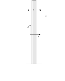
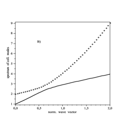
Figure 1: A) Schematic picture of the system under consideration. The thick line between the S and F layers means an insulating layer; B) Spectrum of coupled spin and plasma-like modes. On the vertical and horizontal axes we plot the quantity $(\omega/\Omega_{J})^{2}$, and $(kl_{J})^{2}$, respectively. The following parameters are chosen: $(\Omega_{J}/\Omega_{M})^{2}=2$, $(l_{J}/l_{M})=1$ and $s=0.05$

$$[\mathbf{j}_{\perp}]=(c/4\pi)\lambda_{L}^{-2}\{4\pi\tilde{d}_{F}(\mathbf{n}_{z}\mathbf{\times M}_{\perp})+(\Phi_{0}/2\pi)\mathbf{\nabla}_{\perp}\varphi\}$$ (2)

where $\tilde{d}_{F}=d_{F}$ (or $2d_{F}$) in the case of a SIFS (or SFIFS) junction, $d_{F}$ is the thickness of the F film which is assumed to be smaller than the London penetration length $\lambda_{L}$. This assumption allows one to neglect the change of $\mathbf{A}_{\perp}$ caused by Meissner currents in the F layer and to write the change of the vector potential $\mathbf{A}_{\perp}$ in the form $[\mathbf{A}_{\perp}]=\tilde{d}_{F}(\mathbf{n}_{z}\mathbf{\times\mathbf{B}_{\perp}})$ with $\mathbf{\mathbf{B}_{\perp}}=4\pi\mathbf{M}_{\perp}+\mathbf{H}_{\perp}$.

We proceed by solving the London equation in the superconductors with boundary conditions determined by the change of the current density (see, e.g., AV ). A solution of this equation for S films with the thickness exceeding $\lambda_{L}$ takes the form

$$\mathbf{B}_{\perp}(z)=\{\frac{\Phi_{0}}{4\pi\lambda_{L}}\mathbf{n}_{z}\mathbf{\times\nabla}_{\perp}\varphi-\frac{2\pi\tilde{d}_{F}}{\lambda_{L}}\mathbf{M}_{\perp}\}\exp(-\frac{(|z|-d_{F})}{\lambda_{L}}).$$ (3)

Eq. (3) describes the penetration of the magnetic induction into the superconductors ($|z|>d_{F}$). It is well known that the magnetic field penetrates the JJ in a form of fluxons Josephson ; Barone . Eq. (3) supports this picture for the SFIFS junctions. Integrating Eq. (3) over $z$ and $x$ and adding the magnetic flux in the F film $\Phi_{F}=4\pi\tilde{d}_{F}L_{x}M_{y}$ (the magnetic moment $M_{\perp}$ is assumed to be oriented in the $y$ direction), we come to flux quantization: $\Phi=$ $(\Phi_{0}n),$ where $n=[\varphi]_{x}/2\pi$ is the number of fluxons and $[\varphi]_{x}$ is the phase variation on the length $L_{x}$, which is supposed to be an integer multiple of $2\pi.$

In order to obtain an equation for the phase difference $\varphi$, we use the Maxwell equation $(\mathbf{\nabla\times B)}_{z}=(4\pi/c)j_{z}$ in the superconductors and the standard expression for the Josephson current. Then, we obtain

$$\Omega_{J}^{-2}(\frac{\partial^{2}\varphi}{\partial t^{2}}\mathbf{+}\gamma_{J}\frac{\partial\varphi}{\partial t})-l_{J}^{2}\mathbf{\nabla}_{\perp}^{2}\varphi+\sin\varphi=\eta-\frac{c\tilde{d}_{F}}{2\lambda_{L}j_{c}}(\mathbf{\nabla\times M}_{\perp})_{z}$$ (4)

where $\Omega_{J}=(2ej_{c}/C_{\square}\hbar)^{1/2}$ is the Josephson “plasma” frequency, $\gamma=(R_{\square}C_{\square})^{-1}$, $C_{\square}=\epsilon/4\pi d$ and $R_{\square}$ are the capacitance and resistance of the junction per unit area, $d$ is the thickness of the insulating layer, $l_{J}^{2}=v_{J}^{2}/\Omega_{J}^{2},$ $v_{J}=c\sqrt{d/2\epsilon\lambda_{L}}$ is the velocity of the plasma wave propagation (Swihart waves). The first term on the r.h.s. of Eq. (4) , $\eta=j/j_{c}$, is the normalized current through the junction. A simpler equation for the stationary case has been written previously in Ref. AV , where a similar system with a multidomain ferromagnet was considered.

The dynamics of the magnetization in the F layer is described by the well known equation with account for the magnetic induction due to the Meissner currents (see for example Ref. Sonin )

$$\frac{\partial\mathbf{M}_{\perp}}{\partial t}=-4\pi g\alpha(1-\tilde{l}_{M}^{2}\mathbf{\nabla}_{\perp}^{2})(\mathbf{M\times M}_{\perp})+g\mathbf{M\times B}_{\perp}$$ (5)

where $g$ is the gyromagnetic factor, $\alpha$ is a parameter related to the anisotropy constant $\beta=(\alpha-1)$, $\tilde{l}_{M}$ is a characteristic length related to the spin waves.

We further substitute $\mathbf{B}_{\perp F}=4\pi\mathbf{M}_{\perp}+\mathbf{B}_{\perp S}(d_{F})$ into Eq. (5), where $\mathbf{B}_{\perp F}$ is the magnetic induction in the F layer and $\mathbf{B}_{\perp S}=\mathbf{B}_{\perp}(z\rightarrow d_{F})$ is given by Eq.(3). Finally we come to the equation

$$-\frac{\partial\mathbf{M}_{\perp}}{\partial t}=\Omega_{M}[\frac{\mathbf{M\times M}_{\perp}}{M_{0}}(1+s-l_{M}^{2}\mathbf{\nabla}_{\perp}^{2})+\frac{\Phi_{0}}{(4\pi)^{2}\beta\lambda_{L}}\mathbf{\nabla}_{\perp}\varphi]$$ (6)

where $\Omega_{M}=4\pi gM_{0}\beta=4\pi gM_{0}(\alpha-1)$ is the resonance frequency of the magnetic moment precession ($\alpha>1$), $s=\tilde{d}_{F}/(2\beta\lambda_{L}),$ $l_{M}^{2}=(\alpha/(\alpha-1))\tilde{l}_{M}^{2}$. One could also take into account a damping adding to the r.h.s. of Eq. (6) the term $\gamma_{M}(\mathbf{M}\times\partial\mathbf{M}/\partial t)/M$ ($\gamma_{M}$ is the dimensionless Gilbert constant).

Eqs. (4, 6) are the final equations fully describing dynamics of the SFIFS junctions. The most interesting effect that we will obtain now is the hybridization of charge and spin excitations resulting in a new collective hybridized mode.

a) Hybridized mode. Let us consider the simplest monodomain case when the magnetization $\mathbf{M_{0}}$ is normal to the interface, so that in equilibrium $B_{0}=0$. Small perturbations near the equilibrium result in a precession of the magnetic moment $\mathbf{M}$ and in a variation of the phase difference $\varphi$ in time and space. Representing $\mathbf{M}$ for small deviations $\mathbf{m}_{\perp}$ as $\mathbf{M=}M_{0}\mathbf{n}_{z}+\mathbf{m}_{\perp}$, we can linearize Eqs. (6) and (4). A nonzero solution of these linearized equations exists provided the determinant of these two equations equals zero. Writing the perturbations in the form of plane waves ($\mathbf{m}_{\perp}\sim\varphi\sim\exp(i\omega t+i\mathbf{kr}_{\perp}))$ and setting the determinant to zero we come to the dispersion relation

$$[\omega^{2}-\Omega_{M}^{2}(k)][\omega^{2}-\Omega_{J}^{2}(k)]=s\Omega_{M}(k)\Omega_{M}v_{J}^{2}k^{2}$$ (7)

where $\Omega_{M}^{2}(k)=\Omega_{M}^{2}(1+s+(kl_{M})^{2})^{2},$ $\Omega_{J}^{2}(k)=\Omega_{J}^{2}(1+(kl_{J})^{2}).$ For simplicity, we neglected the damping setting $\gamma_{M}\rightarrow 0.$

Eq. (7) describes the spectrum of the hybridized mode. This mode decouples into the spin and charge excitations only in the limit when the right hand side can be neglected. In this case the spin waves with the spectrum $\Omega_{M}(k)$ and the plasma-like Josephson waves with the spectrum $\Omega_{J}(k)$ exist separately. In the general case we have the coupled spin wave and plasma-like modes in the system. The most interesting behavior corresponds to the case $\Omega_{M}<\Omega_{J}$. In this situation, the two branches of the spectrum cross each other in the absence of the coupling and the coupling leads to a mutual repulsion of these branches. In Fig. 1b we show the dependence $\omega(k)$ just for this case. Note that the frequency of the considered collective modes remains unchanged by inversion of the magnetization direction, $M\leftrightarrow-M$, that is, in a multidomain case we would obtain the same dependence $\omega(k).$ 

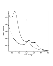
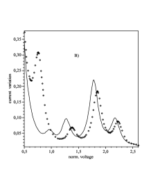
Figure 2: Correction to the I-V characteristics due to interaction of Josephson oscillations and collective modes. The normalized voltage is defined as $V_{norm}=\Omega_{V}/\Omega_{J}.$ Solid curves correspond to a small parameter $s\equiv 2(\tilde{d}_{F}/\beta\lambda_{L})=0.05$ (negligible effect of the F layer), point curves correspond to $s=0.4.$ The plots are presented for the following parameters: A) $\Omega_{M}/\Omega_{J}=2,$ $\kappa_{H}l_{J}=2;$ B) $\Omega_{M}/\Omega_{J}=1,$ $\kappa_{H}l_{J}=4.$ The damping coefficients are $\gamma_{J}/\Omega_{J}=0.2,\gamma_{M}/\Omega_{J}=0.1.$

The collective modes in the Josephson junctions can be excited by the internal Josephson oscillations. It is well known that the interaction of Josephson oscillations with plasma-like waves in a tunnel Josephson junction in the presence of a weak external magnetic field leads to Fiske steps on the I-V characteristics (see, e.g., Refs. Barone , EckKulik ). In the next paragraph we consider the modification of Fiske steps in tunnel SFIFS or SIFS junctions due to the hybridization of the collective modes using Eqs. (4, 6).

b) Fiske steps. We assume again that the magnetization $M$ is oriented perpendicular to the interfaces and a small external magnetic field $H_{e}$ is applied parallel to the films. It is important to have in mind that the magnetization $M_{0}$ is of the order of $100\mathit{Gauss}$ or larger, whereas $H_{e}$ is about a few $\mathit{Gauss}$. Therefore one can neglect the in-plane magnetization $M_{y}=H_{e}/4\pi\beta$ in comparison with $M_{0}$. We assume also that the length of the junction along the $x-$axis is shorter than the Josephson length $l_{J}$.

In this limit the phase $\varphi$ can be represented in the form (see Refs. EckKulik ): $\varphi=\varphi_{0}(x,t)+\psi(x,t)$ with $\varphi_{0}(x,t)=\Omega_{V}t+\kappa_{H}x$ and $\Omega_{V}=2eV/\hbar,$ $\kappa_{H}=4\pi\lambda_{L}H_{e}/\Phi_{0}$. Linearizing Eq. (4) we obtain the equation for $\psi$

$$\Omega_{J}^{-2}(\frac{\partial^{2}\psi}{\partial t^{2}}\mathbf{+}\gamma\frac{\partial\psi}{\partial t})-l_{J}^{2}\frac{\partial^{2}\psi}{\partial x^{2}}=-\sin\varphi_{0}-\frac{c\tilde{d}_{F}}{2\lambda_{L}j_{c}}\frac{\partial m_{y}}{\partial x}$$ (8)

The dc current is $\eta=(2eV\gamma/\hbar)/\Omega_{J}+\langle\psi(x,t)\cos\varphi_{0}(x,t)\rangle,$ where the angular brackets denote the averaging in space and time. The derivative $\partial m_{y}/\partial x$ can be found from Eq. (6) with $\varphi$ replaced by $\psi.$ The first term on the right-hand side in Eq. (8) plays a role of an external force oscillating in space and time and acting on a resonance system. This equation should be solved using boundary conditions $\partial\psi/\partial x=0$ at $x=\pm L_{x}/2.$ Carrying out these calculations we obtain a contribution $\delta\eta\equiv\langle\psi(x,t)\cos\varphi_{0}(x,t)\rangle$ to the current originating from the collective modes

$$\delta\eta=\frac{1}{2}Im\{\frac{1}{\mathit{D}}[1-\frac{\theta_{H}^{2}}{\theta_{V}}\frac{\cos(2\theta_{V})-\cos(2\theta_{H})}{(\theta_{H}^{2}-\theta_{V}^{2})\sin(2\theta_{V})}]\}$$ (9)

where $\mathit{D}=(\theta_{V}^{2}-\theta_{H}^{2})a_{V}^{2}/\theta_{V}^{2},a_{V}^{2}=(\Omega_{V}^{2}-i\gamma_{J}\Omega_{V})/\Omega_{J}^{2}$, $\theta_{H}=\kappa_{H}L_{x}/2,\theta_{V}=\kappa_{V}L_{x}/2,\kappa_{V}=a_{V}/l_{V},$ $l_{V}=l_{J}[1+s\Omega_{M}^{2}/(\Omega_{V}^{2}-\Omega_{Ms}^{2})]^{1/2},\Omega_{Ms}^{2}=\Omega_{M}^{2}(1+s).$ For simplicity we consider the limit $l_{J}>>l_{M}.$

In Fig.2 we plot the dependence $\delta\eta(V)$ vs the normalized voltage $\Omega_{V}/\Omega_{J}$ for different values of the parameter $s=2\pi\tilde{d}_{F}/(\beta\lambda_{L})$. In order to avoid a divergence, we took into account a finite damping in the F layer replacing $(\Omega_{V}^{2}-\Omega_{Ms}^{2})$ by $(\Omega_{V}(\Omega_{V}-i\gamma_{M})-\Omega_{Ms}^{2})$.

In the limit of small values of $s$ ($s\rightarrow 0$) this dependence describes Fiske steps in the conventional Josephson SIS junction. Solid lines in Figs. 2 correspond to small values of $s$ ($s=0.05$) when the influence of the F layer is negligible and point lines correspond to larger values of $s$ ($s=0.4$). One can see from Fig. 2a that near the frequency of the magnetic resonance, $\Omega_{V}\approx\Omega_{Ms}=2\Omega_{J}$ there is a double peak (point curve), which is absent in junctions with a small $s$ (solid curve). Fig. 2b shows that the presence of the F layer leads not only to a shift of maxima in the dependence $\delta\eta(V)$ but also to a change of the overall form of this dependence.

To conclude, we have developed theory describing electrodynamics of the SFIFS or SIFS tunnel Josephson junctions. In the framework of our approach dynamics of these systems is fully described by Eqs. (4, 6). Solving these equations we found new effects related to hybridization of charge and spin degrees of freedom. We demonstrated that the different branches - Josephson plasma-like and spin wave branch - of the spectrum repel each other. The hybridization of the collective modes results in new interesting peculiarities of the $I-V$ characteristics. We have demonstrated that the positions, shape and number of the Fiske steps arising in the presence of a weak external in-plane magnetic field and an applied voltage $V$ change. In particular, new peaks appear due to excitation of magnetic modes. We believe that on the basis of the SIFS junctions one may construct a new type of spectrometers that would allow one to extract an information about spin excitations in thin ferromagnetic layers. It seems that an experimental observation of the effects predicted here is not very difficult and can be performed by measuring $I-V$ characteristics, spectra of collective excitations, etc., using standard experimental methods developed for studying Josephson junctions.

We thank SFB 491 for financial support.

References

- (1) B. D. Josephson, Rev. Mod. Phys., 36, 216-220 (1964).
- (2) A.Barone and G.Paterno, Physics and applications of the Josephson effect, Wiley, NY (1982).
- (3) A.E. Koshelev and L.N. Bulaevskii, Phys. Rev. B 77, 014530 (2008).
- (4) A. A. Golubov, M. Yu. Kupriyanov, and E. Il’ichev, Rev. Mod. Phys. 76, 411 (2004)
- (5) A. Buzdin, Rev. Mod. Phys. 77, 935 (2005).
- (6) F.S. Bergeret, A.F. Volkov, K.B. Efetov, Rev. Mod. Phys. 77, 1321 (2005).
- (7) I.F. Lyuksyutov and V.L. Pokrovsky, Adv. Phys. 54, 67 (2005).
- (8) M. Eschrig, T. Lofwander, T. Champel, J. C. Cuevas, J. Kopu, Gerd Schön, J. Low Temp. Phys. 147, 457, (2007).
- (9) X. Waintal, P. W. Brouwer, Phys. Rev. B 65, 054407 (2002); I. V. Bobkova and A. M. Bobkov, ibid B 74, 220504 (2006); J. Michelsen, V. S. Shumeiko, and G. Wendin, Phys. Rev. B 77, 184506 (2008); Jian-Xin Zhu, Z. Nussinov, A. Shnirman, and A. V. Balatsky, Phys. Rev. Lett. 92, 107001 (2004); E. Zhao and J. A. Sauls, ibid. 98, 206601 (2007);
- (10) V. Braude and Ya. M. Blanter, Phys. Rev. Lett. 100, 207001 (2008); M. Houzet, ibid 101, 057009 (2008); F. Konschelle and A. Buzdin, ibid 102, 017001 (2009). .
- (11) S. Hikino, M. Mori, S. Takahashi, S. Maekawa, J. Phys. Soc. Jpn. 77, 053707 (2008).
- (12) I.A. Garifullin et al., Appl. Magn. Res. 22, 439 (2002); C. Bell, S. Milikisyants, M. Huber, and J. Aarts, Phys. Rev. Lett. 100, 047002 (2008).
- (13) A.S. Vasenko, A.A. Golubov, M.Yu. Kupriyanov, and M.Weides, Phys. Rev. B 77, 134507 (2008); J. Pfeiffer et al., ibid 77, 214506 (2008).
- (14) V. Braude and E.B. Sonin, Phys. Rev. Lett. 93, 117001 (2004).
- (15) A.F. Volkov and A. Anishchanka, Phys. Rev. B 71, 024501 (2005).
- (16) R. E. Eck, D. J. Scalapino, and B. N. Taylor, Phys. Rev. Lett., 13, 15 (1964); I.O. Kulik, JETP Lett., 2, 134 (1965).