Charged MSSM Higgs Bosons at CMS:
Reach and Parameter Dependence

Abstract:

We review the analysis of the $5\,\sigma$ discovery contours for the charged MSSM Higgs boson at the CMS experiment with 30 $\mbox{fb}^{-1}$ for the two cases $M_{H^{\pm}}<m_{t}$ and $M_{H^{\pm}}>m_{t}$. Latest results for the CMS experimental sensitivities based on full simulation studies are combined with state-of-the-art theoretical predictions of MSSM Higgs-boson production and decay properties. Special focus is put on the SUSY parameter dependence of the $5\,\sigma$ contours. The variation of $\mu$ can shift the prospective discovery reach in $\tan\beta$ by up to $\Delta\tan\beta~{}=~{}40$. We furthermore discuss various theory uncertainties on the signal cross section and branching ratio calculations. In order to arrive at a reliable interpretation of a signal of the charged MSSM Higgs boson at the LHC a strong reduction in the relevant theory uncertainties will be necessary.

1 Introduction

One of the main goals of the LHC is the identification of the mechanism of electroweak symmetry breaking. The most frequently investigated models are the Higgs mechanism within the Standard Model (SM) and within the Minimal Supersymmetric Standard Model (MSSM). Contrary to the case of the SM, in the MSSM two Higgs doublets are required. This results in five physical Higgs bosons. These are the light and heavy ${\cal CP}$-even Higgs bosons, $h$ and $H$, the ${\cal CP}$-odd Higgs boson, $A$, and the charged Higgs bosons, $H^{\pm}$. The Higgs sector of the MSSM can be specified at lowest order in terms of the gauge couplings, the ratio of the two Higgs vacuum expectation values, $\tan\beta\equiv v_{2}/v_{1}$, and the mass of the ${\cal CP}$-odd Higgs boson, $M_{A}$. Consequently, the masses of the ${\cal CP}$-even neutral and the charged Higgs bosons as well as their production and decay characteristics are dependent quantities that can be predicted in terms of the Higgs-sector parameters, e.g. $M_{H^{\pm}}^{2}=M_{A}^{2}+M_{W}^{2}$, where $M_{W}$ denotes the mass of the $W$ boson. Such tree-level results in the MSSM are strongly affected by higher-order corrections, in particular from the sector of the third generation quarks and squarks, so that the dependencies on various other MSSM parameters can be important, see e.g. Ref. [1] for reviews.

Here we review [2] the $5\,\sigma$ charged MSSM Higgs discovery contours at the LHC for the two cases $M_{H^{\pm}}<m_{t}$ and $M_{H^{\pm}}>m_{t}$ within the ${\cal CP}$-conserving $m_{h}^{\rm max}$ scenario [3, 4]. The results are displayed in the $M_{H^{\pm}}$–$\tan\beta$ plane. The respective LHC analyses are given in Ref. [5] for ATLAS and in Refs. [6, 7] for CMS. However, within these analyses the variation with relevant SUSY parameters as well as possibly relevant loop corrections in the Higgs production and decay [4] have been neglected. Earlier analyses can be found in Ref. [8].

2 Combined analysis

The analysis of the variation with respect to the relevant SUSY parameters of the $5\,\sigma$ discovery contours of the charged Higgs boson has been performed in Ref. [2]. The results have been obtained by using the latest CMS analyses [6, 7] (based on 30 $\mbox{fb}^{-1}$) derived in a model-independent approach, i.e. making no assumption on the Higgs boson production mechanism or decays. However, only SM backgrounds have been considered. These experimental results are combined with up-to-date theoretical predictions for charged Higgs production and decay in the MSSM, taking into account also the decay to SUSY particles that can in principle suppress the branching ratio of the charged Higgs boson decay to $\tau\nu_{\tau}$.

The main production channels at the LHC are

$$pp\to t\bar{t}\;+\;X,\quad t\bar{t}\to t\;H^{-}\bar{b}\mbox{~{}~{}or~{}~{}}H^{+}b\;\bar{t},$$ (1)

$$gb\to H^{-}t\mbox{~{}~{}or~{}~{}}g\bar{b}\to H^{+}\bar{t}~{}.$$ (2)

The decay used in the analysis to detect the charged Higgs boson is

$$H^{\pm}\;\to\;\tau\nu_{\tau}\;\to\;{\rm hadrons~{}}\nu_{\tau}.$$ (3)

The g“light charged Higgs boson” is characterized by $M_{H^{\pm}}<m_{t}$. The main production channel is given in eq. (1). Close to threshold also eq. (2) contributes. The relevant (i.e. detectable) decay channel is given by eq. (3). The experimental analysis is based on 30 $\mbox{fb}^{-1}$ collected with CMS. The events were required to be selected with the single lepton trigger, thus exploiting the $W\to\ell\nu$ decay mode of a $W$ boson from the decay of one of the top quarks in eq. (1). More details can be found in Refs. [6, 2].

The g“heavy charged Higgs boson” is characterized by $M_{H^{\pm}}\;\raisebox{-3.00003pt}{$\stackrel{{\scriptstyle\displaystyle>}}{{\sim}}$}\;m_{t}$. Here eq. (2) gives the largest contribution to the production cross section, and very close to threshold eq. (1) can contribute somewhat. The relevant decay channel is again given in eq. (3). The experimental analysis is based on 30 $\mbox{fb}^{-1}$ collected with CMS. The fully hadronic final state topology was considered, thus events were selected with the single $\tau$ trigger at Level-1 and the combined $\tau$-$E_{\rm T}^{\rm miss}$ High Level trigger. The backgrounds considered were $t\bar{t}$, $W^{\pm}t$, $W^{\pm}+3~{}{\rm jets}$ as well as QCD multi-jet background [9, 10, 11]. The production cross sections for the $t\bar{t}$ background processes were normalized to the NLO cross sections [12]. More details can be found in Refs. [7, 2].

For the calculation of cross sections and branching ratios we use a combination of up-to-date theory evaluations. The interaction of the charged Higgs boson with the $t/b$ doublet can be expressed in terms of an effective Lagrangian [13],

$${\cal L}=\frac{g}{2M_{W}}\frac{\overline{m}_{b}}{1+\Delta_{b}}\Bigg{[}\sqrt{2}\,V_{tb}\,\tan\beta\;H^{+}\bar{t}_{L}b_{R}\Bigg{]}+{\rm h.c.}$$ (4)

Here $\overline{m}_{b}$ denotes the running bottom quark mass including SM QCD corrections. $\Delta_{b}\propto\mu\tan\beta$ depends on the scalar top and bottom masses, the gluino mass, the Higgs mixing parameter $\mu$ and $\tan\beta$. The explicit expression can be found in Refs. [14, 4].

For the production cross section in eq. (1) we use the SM cross section $\sigma(pp\to t\bar{t})=840~{}\rm{pb}$ [12] times the ${\rm BR}(t\to H^{\pm}\,b)$ including the $\Delta_{b}$ corrections described above. The production cross section in eq. (2) is evaluated as given in Ref. [15]. In addition also the $\Delta_{b}$ corrections of eq. (4) are applied. Finally the ${\rm BR}(H^{\pm}\to\tau\nu_{\tau})$ is evaluated taking into account all decay channels, among which the most relevant are $H^{\pm}\to tb,cs,W^{(*)}h$. Also possible decays to SUSY particles are considered. For the decay to $tb$ again the $\Delta_{b}$ corrections are included. All the numerical evaluations are performed with the program FeynHiggs [16], see also Refs. [17, 18].

3 Numerical results

The numerical analysis has been performed [2] in the $m_{h}^{\rm max}$ scenario [3, 4] for $\mu=-1000$, -200, +200, $+1000\,\,\mathrm{GeV}$. In Fig. 1 we show the results for the variation of the $5\,\sigma$ discovery contours for the light (left plot) and the heavy (right plot) charged Higgs boson, where the charged Higgs boson discovery will be possible in the areas above the curves shown in the figure. The top quark mass is set to $m_{t}=175\,\,\mathrm{GeV}$. The thick (thin) lines correspond to positive (negative) $\mu$, and the solid (dotted) lines have $|\mu|=1000(200)\,\,\mathrm{GeV}$.

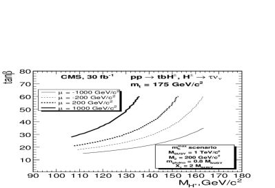
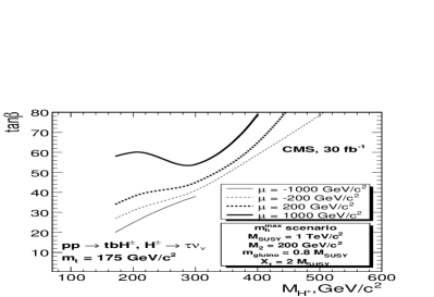
Figure 1: Discovery reach for the light (left) and heavy (right) charged Higgs boson in the $M_{H^{\pm}}$–$\tan\beta$ plane for the $m_{h}^{\rm max}$ scenario [2].

Concerning the light charged Higgs case, the curves stop at $\tan\beta=60$, where we stopped the evaluation of production cross section and branching ratios. For negative $\mu$ very large values of $\tan\beta$ result in a strong enhancement of the bottom Yukawa coupling, and for $\Delta_{b}\to-1$ the MSSM enters a non-perturbative regime, see eq. (4). The search for the light charged Higgs boson covers the area of large $\tan\beta$ and $M_{H^{\pm}}\;\raisebox{-3.00003pt}{$\stackrel{{\scriptstyle\displaystyle<}}{{\sim}}$}\;130\ldots 160\,\,\mathrm{GeV}$. The variation with $\mu$ induces a strong shift in the $5\,\sigma$ discovery contours. This corresponds to a shift in $\tan\beta$ of $\Delta\tan\beta=15$ for $M_{H^{\pm}}\;\raisebox{-3.00003pt}{$\stackrel{{\scriptstyle\displaystyle<}}{{\sim}}$}\;110\,\,\mathrm{GeV}$, rising up to $\Delta\tan\beta=40$ for larger $M_{H^{\pm}}$ values. The discovery region is largest (smallest) for $\mu=-(+)1000\,\,\mathrm{GeV}$, corresponding to the largest (smallest) production cross section.

We now turn to the heavy charged Higgs case. For $M_{H^{\pm}}=170\,\,\mathrm{GeV}$, where the experimental analysis stops, we find a strong variation in the accessible parameter space for $\mu=-(+)1000\,\,\mathrm{GeV}$ of $\Delta\tan\beta=40$. It should be noted in this context that close to threshold, where both production mechanisms, eqs. (1) and (2), contribute, the theoretical uncertainties are somewhat larger than in the other regions. Furthermore, for relatively low $M_{H^{\pm}}$ the compensation of the $\Delta_{b}$ effects from production and decay is not strong, leading to a larger variation with $\Delta_{b}$. For $M_{H^{\pm}}=300\,\,\mathrm{GeV}$ the variation in the $5\,\sigma$ discovery contours goes from $\tan\beta=38$ to $\tan\beta=54$. For $\mu=-1000\,\,\mathrm{GeV}$ and larger $\tan\beta$ values the bottom Yukawa coupling becomes so large that a perturbative treatment would no longer be reliable in this region, and correspondingly we do not continue the respective curve(s). Detailed explanations about the shape of the $\mu=+1000\,\,\mathrm{GeV}$ curve for $M_{H^{\pm}}\approx 300\,\,\mathrm{GeV}$ can be found in Ref. [2].

  

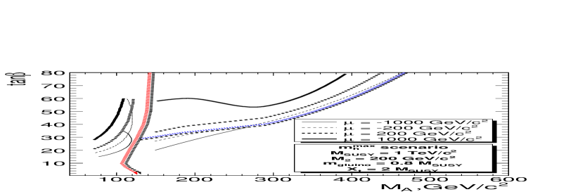
Figure 2: Discovery reach for the charged Higgs boson of CMS with 30 $\mbox{fb}^{-1}$ in the $M_{A}$–$\tan\beta$ plane for the $m_{h}^{\rm max}$ scenario for $\mu=\pm 200,\pm 1000\,\,\mathrm{GeV}$ in comparison with the results from the CMS PTDR [19] (see text), obtained for $\mu=+200\,\,\mathrm{GeV}$ and neglecting the $\Delta_{b}$ effects [2].

In Fig. 2 we show the combined results for the $5\,\sigma$ discovery contours for the light and the heavy charged Higgs boson, corresponding to the experimental analyses in the $m_{h}^{\rm max}$ scenario. They are compared with the results presented in the CMS PTDR [19], now shown in the $M_{A}$–$\tan\beta$ plane. The thick (thin) lines correspond to positive (negative) $\mu$, and the solid (dotted) lines have $|\mu|=1000(200)\,\,\mathrm{GeV}$. The thickened dotted (red/blue) lines represent the CMS PTDR results, obtained for $\mu=+200\,\,\mathrm{GeV}$ and neglecting the $\Delta_{b}$ effects. Apart from the variation in the $5\,\sigma$ discovery contours with the size and the sign of $|\mu|$, two differences can be observed in the comparison with the PTDR results. For the light charged Higgs analysis the discovery contours are now shifted to smaller $M_{A}$ values, for negative $\mu$ even “bending over” for larger $\tan\beta$ values. The reason is the more complete inclusion of higher-order corrections to the relation between $M_{A}$ and $M_{H^{\pm}}$ that is included in FeynHiggs as compared to the calculation used for the CMS PTDR. The second feature is a small gap between the light and the heavy charged Higgs analyses, while in the PTDR analysis all charged Higgs masses could be accessed. Possibly the heavy charged Higgs analysis strategy exploiting the fully hadronic final state can be extended to smaller $M_{A}$ values to completely close the gap. For the interpretation of Fig. 2 it should be kept in mind that the accessible area in the heavy Higgs analysis also “bends over” to smaller $M_{A}$ values for larger $\tan\beta$, thus decreasing the visible gap in Fig. 2.

4 Theory uncertainties

The prediction of the charged Higgs production cross section is subject to theory uncertainties, $\sim 6.5\%$ in the low mass case and $\;\raisebox{-3.00003pt}{$\stackrel{{\scriptstyle\displaystyle<}}{{\sim}}$}\;20\%$ in the high charged Higgs mass range, see Ref. [2] for details and a complete list of references. Furthermore the ${\cal O}(\alpha_{s})$ corrections entering via $\Delta_{b}$ have been estimated to yield an intrinsic uncertainty of $\;\raisebox{-3.00003pt}{$\stackrel{{\scriptstyle\displaystyle<}}{{\sim}}$}\;20\%$. These theory errors have an effect on the $5\,\sigma$ discovery contours analyzed in the previous section. In Fig. 3 we show the corresponding $5\,\sigma$ discovery contours as a function of $M_{H^{\pm}}$ in the case of low (high) $M_{H^{\pm}}$ in the left (right) plot. The dark (light) shaded band have been obtained for positive (negative) $\mu$, and the solid lines represent the central values. In the low $M_{H^{\pm}}$ case the two bands show substantial overlap, separating only for the highest $M_{H^{\pm}}$ values. In the high $M_{H^{\pm}}$ case the two bands overlap for $M_{H^{\pm}}\;\raisebox{-3.00003pt}{$\stackrel{{\scriptstyle\displaystyle>}}{{\sim}}$}\;280\,\,\mathrm{GeV}$. This shows that the effects of the current level of theory uncertainties can be at the same level as the effect of the variation of the sign and size of $\mu$.

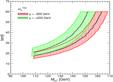
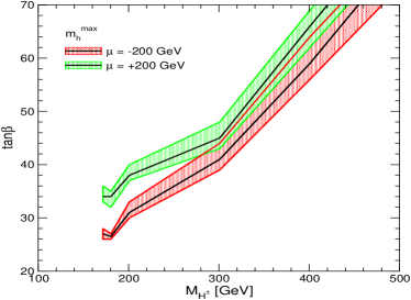
Figure 3: The $5\,\sigma$ discovery contours as a function of $M_{H^{\pm}}$ including theory uncertainties (see text).

Consequently, turning the argument around and assuming a charged Higgs boson signal at the LHC, the theory uncertainties play an important role. In order to arrive at a reliable interpretation of a signal of the charged MSSM Higgs boson at the LHC a strong reduction in the relevant theory uncertainties as outlined above is necessary. Only then an analysis in terms of underlying model parameters can be performed.

Acknowledgements

We thank the organizers of cH${}^{\mbox{}^{\pm}}$arged 2008 for the invitation and the stimulating atmosphere. Work supported in part by the European Community’s Marie-Curie Research Training Network under contract MRTN-CT-2006-035505 ‘Tools and Precision Calculations for Physics Discoveries at Colliders’.

References

- [1] S. Heinemeyer, W. Hollik and G. Weiglein, Phys. Rept. 425 (2006) 265; S. Heinemeyer, Int. J. Mod. Phys. A 21 (2006) 2659; A. Djouadi, Phys. Rept. 459 (2008) 1.
- [2] M. Hashemi et al., arXiv:0804.1228 [hep-ph];
- [3] M. Carena et al., Eur. Phys. J. C 26 (2003) 601.
- [4] M. Carena et al., Eur. Phys. J. C 45 (2006) 797.
- [5] K. Assamagan, Y. Coadou and A. Deandrea, Eur. Phys. J. direct C 4 (2002) 9; K. Assamagan and N. Gollub, Eur. Phys. J. C 39S2 (2005) 25.
- [6] M. Baarmand, M. Hashemi and A. Nikitenko, CMS Note 2006/056.
- [7] R. Kinnunen, CMS Note 2006/100.
- [8] J. Coarasa et al., Eur. Phys. J. C 2 (1998) 373; A. Belyaev et al., Phys. Rev. D 65 (2002) 031701; JHEP 0206 (2002) 059; K. Assamagan et al., arXiv:hep-ph/0402212; Czech. J. Phys. 55 (2005) B787.
- [9] W. Long and T. Stelzer, Comput. Phys. Commun. 81 (1994) 357; F. Maltoni and T. Stelzer, JHEP 0302 (2003) 027.
- [10] T. Sjostrand et al., Comput. Phys. Commun. 135 (2001) 238.
- [11] S. Slabospitsky and L. Sonnenschein, Comput. Phys. Commun. 148 (2002) 87.
- [12] P. Nason, S. Dawson and R. K. Ellis, Nucl. Phys. B 303 (1988) 607; W. Beenakker et al., Phys. Rev. D 40 (1989) 54; M. Beneke et al., arXiv:hep-ph/0003033, and references therein.
- [13] M. Carena et al., Nucl. Phys. B 577 (2000) 577.
- [14] R. Hempfling, Phys. Rev. D 49 (1994) 6168; L. Hall, R. Rattazzi and U. Sarid, Phys. Rev. D 50 (1994) 7048; M. Carena et al., Nucl. Phys. B 426 (1994) 269.
- [15] T. Plehn, Phys. Rev. D 67 (2003) 014018; E. Berger et al., Phys. Rev. D 71 (2005) 115012.
- [16] S. Heinemeyer, W. Hollik and G. Weiglein, Comput. Phys. Commun. 124 (2000) 76; Eur. Phys. J. C 9 (1999) 343; G. Degrassi et al., Eur. Phys. J. C 28 (2003) 133; M. Frank et al., JHEP 0702 (2007) 047; see: www.feynhiggs.de .
- [17] S. Heinemeyer et al., Phys. Lett. B 652 (2007) 300.
- [18] S. Heinemeyer, arXiv:0812.0523 [hep-ph];
- [19] CMS Collaboration, Physics Technical Design Report, Volume 2. CERN/LHCC 2006-021, see: cmsdoc.cern.ch/cms/cpt/tdr/ .