Field theory of bicritical and tetracritical points. III. Relaxational dynamics including conservation of magnetization (Model C)

Abstract

We calculate the relaxational dynamical critical behavior of systems of $O(n_{\|})\oplus O(n_{\perp})$ symmetry including conservation of magnetization by renormalization group (RG) theory within the minimal subtraction scheme in two loop order. Within the stability region of the Heisenberg fixed point and the biconical fixed point strong dynamical scaling holds with the asymptotic dynamical critical exponent $z=2\phi/\nu-1$ where $\phi$ is the crossover exponent and $\nu$ the exponent of the correlation length. The critical dynamics at $n_{\|}=1$ and $n_{\perp}=2$ is governed by a small dynamical transient exponent leading to nonuniversal nonasymptotic dynamical behavior. This may be seen e.g. in the temperature dependence of the magnetic transport coefficients.

I Introduction

In two preceding paperspartI ; partII we have considered the critical statics and relaxational dynamics of $O(n_{\|})\oplus O(n_{\perp})$ physical systems near the multicritical point where the two phase transition lines of the system corresponding to $O(n_{\|})$-symmetry and $O(n_{\perp})$-symmetry meet. The space of the order parameter (OP) dimensions $n_{\|}$ and $n_{\perp}$ decomposes in regions where the multicritical behavior is described by different fixed points (FPs) - the $O(n=n_{\|}+n_{\perp})$- isotropic FP, the biconical FP, the decoupling FP - and a region where no stable FP is found (run away region) (see Fig 1 in Ref.partI ). In the resummed two loop order field theoretic treatment it was found that for integer values of $n_{\|}$ and $n_{\perp}$ the biconical FP is stable only for a system with $n_{\|}=1$, $n_{\perp}=2$, and its symmetric counterpart. For specific initial conditions of the nonuniversal parameters of the system also the $O(n=n_{\|}+n_{\perp})$- isotropic FP (Heisenberg FP) might be reached. Such a system is physically represented by an antiferromagnet in an external magnetic field. The two cases mentioned above correspond to tetracritical and bicritical multicritical points correspondingly. If no FP is reached the multicritical point might be of first order, i.e. a triple point.

The dynamics of the antiferromagnet in a magnetic field is quite complicated and the equations of motion have been formulated for the slow densities by Dohm and Janssendohmjanssen77 . These Eqs. contain reversible and irreversible coupling terms between the OPs (the components of the staggered magnetization parallel and perpendicular to the magnetic field) and one conserved density (the parallel component of the magnetization). In fact there is a second conserved density (CD) - the energy density - which in general should be taken into account but it will not be included here since in two loop order the specific heat exponent at the biconical FP turned out to be negative rem1 for the case $n_{\|}=1$ and $n_{\perp}=2$. Concerning the new static resultspartI a simplified dynamical modeldohmjanssen77 has been reconsideredpartII consisting of two relaxational equations for the two OP. The timescale ratio $v$ between the two relaxation rates $\Gamma_{\|}$ and $\Gamma_{\perp}$ introduces a very small dynamical transient since the dynamical FP lies very near to the stability boundary separating strong and weak dynamical scaling. The strong dynamical scaling FP is governed by $v^{\star}$ finite and different from zero whereas the weak dynamical scaling FP by $v^{\star}=0\,\mbox{or}\,\infty$ correspondingly.

A further step to the complete model is to include the diffusive dynamics of the slow CD leading to a model C like extension. In this extended model a new timescale ratio appears defined by the ratio of one of the OP-relaxation rate to the kinetic coefficient $\lambda$ of the conserved density $m$. This model has been studied in one loop order in Refs dohmjanssen77 ; dohmKFA ; dohmmulti83 taking into account only a part of dynamical two loop order terms and one loop statics. Here we present a complete two loop order calculations.

The inclusion of further densities beside the OP makes it necessary to extend the static functional of the usual $\phi^{4}$-theory, although the OP alone would be sufficient to describe the static critical behavior. Such an extended static functional for isotropic systems ($O(n)$ symmetry) with short range interaction has the form hahoma74 ; fomoprl03

$${\cal H}^{(C)}\!=\!\int\!d^{d}x\Bigg{\{}\frac{1}{2}\mathring{\tilde{r}}\vec{\phi}_{0}\cdot\vec{\phi}_{0}+\frac{1}{2}\sum_{i=1}^{n}\nabla_{i}\vec{\phi}_{0}\cdot\nabla_{i}\vec{\phi}_{0}+\frac{1}{2}m_{0}^{2}$$

$$+\frac{\mathring{\tilde{u}}}{4!}\Big{(}\vec{\phi}_{0}\cdot\vec{\phi}_{0}\Big{)}^{2}+\frac{1}{2}\mathring{\gamma}m_{0}\vec{\phi}_{0}\cdot\vec{\phi}_{0}-\mathring{h}m_{0}\Bigg{\}}\ .$$ (1)

Here the order parameter $\vec{\phi}_{0}\equiv\vec{\phi}_{0}(x)$ is assumed to be a $n$-component real vector, the symbol $\cdot$ denotes the scalar product. The secondary density $m_{0}\equiv m_{0}(x)$ is considered as a scalar quantity and $\mathring{h}$ is the conjugated field to $m_{0}$. It is chosen to have a vanishing average value $\langle m_{0}\rangle=0$. Within statics, the above functional is equivalent to the Ginzburg-Landau-Wilson(GLW)-functional

$${\cal H}_{GLW}\!=\!\int\!d^{d}x\Bigg{\{}\frac{1}{2}\mathring{r}\vec{\phi}_{0}\cdot\vec{\phi}_{0}+\frac{1}{2}\sum_{i=1}^{n}\nabla_{i}\vec{\phi}_{0}\cdot\nabla_{i}\vec{\phi}_{0}$$

$$+\frac{\mathring{u}}{4!}\Big{(}\vec{\phi}_{0}\cdot\vec{\phi}_{0}\Big{)}^{2}\Bigg{\}}\ ,$$ (2)

where $\mathring{r}$ is proportional to the temperature distance to the critical point and $\mathring{u}$ is the fourth order coupling in which perturbation expansion is usually performed. The GLW-functional (I) is obtained by integrating out the CD, which appears only in Gaussian order in (I), in the corresponding partition function. The parameters $\mathring{\tilde{r}}$, $\mathring{\tilde{u}}$ and $\mathring{\gamma}$ in (I) and, $\mathring{r}$ and $\mathring{u}$ in (I) are related by

$$\mathring{r}=\mathring{\tilde{r}}+\mathring{\gamma}\mathring{h}\ ,\qquad\mathring{u}=\mathring{\tilde{u}}-3\mathring{\gamma}^{2}\ .$$ (3)

The extended static functional appears in the driving force of the equations of motion for the OP $\vec{\phi}_{0}$ and the CD $m_{0}$. The ratio of the kinetic coefficient $\mathring{\Gamma}$ in the relaxation equation for the OP and the kinetic coefficient $\mathring{\lambda}$ in the diffusive equation for the CD defines the dynamical parameter $w$ whose FP value governs the dynamical scaling of the model.

It is worthwhile to summarize some results for model C at a usual critical point, where the CD can be identified with an energy like density and the value of specific heat exponent $\alpha$ (in any case) governs the relevance of the asymmetric static coupling $\mathring{\gamma}$ between the OP and the CD. Namely, this coupling is irrelevant in the RG sense - it vanishes at the FP - if the specific heat exponent is negative, i.e. the specific heat of the system does not diverge at the critical point. If the specific heat diverges then there remain two possibilities for the dynamical FP: either the FP value of the time scale ratio $w$ between the timescale of the OP and the CD is different from zero and finite, or its FP value is zero or infinite. In the first case strong dynamical scaling with one timescale for the OP and the CD is realized with one dynamical scaling exponent $z=2+\alpha/\nu$ ($\nu$ the exponent of the correlation length). In the second case weak dynamical scaling is present and the time scale of the OP is different from the timescale of the CD, both represented by a corresponding dynamical critical exponent. This region of the weak dynamical scaling FP is tiny (see e.g Fig. 1 in Ref.fomoprl03 ). One should note that at the usual critical point an asymmetric coupling to the OP as given in Eq. (I) is always ’energy-like’ independent of its physical origin. That means the divergence of the CD susceptibility is always described by the specific heat exponent $\alpha$.

In the case of a multicritical point treated here the situation is more complicated since there are two OPs and a CD might couple to both of these OPs. As has been shown in paper I after a proper rotation (Eq. (64)) in the OP space temperature and magnetic like field directions can be identified. In consequence at the multicritical point one has to discriminate the case of energy and magnetization conservation.

The paper is organized as follows. In section II we extend model C of the $O(n)$ symmetrical critical system to the case of a $O(n_{\|})\oplus O(n_{\perp})$ symmetrical multicritical point as considered in papers I and II. The renormalization is performed in section III and the field theoretic functions are calculated in section IV. Then we discuss the possible FP and their stability in section V. Effective dynamical critical behavior is considered in section VI followed in section VII by a short summary of the results and an outlook on further work to be done.

II Model C for multicritical points

II.1 Static functional

In order to describe the multicritical behavior the $n$-dimensional space of the order parameter components is split into two subspaces with dimensions $n_{\perp}$ and $n_{\|}$ with the property $n_{\perp}+n_{\|}=n$. The order parameter separates into

$$\vec{\phi}_{0}=\left(\begin{array}[]{c}\vec{\phi}_{\perp 0}\\ \vec{\phi}_{\|0}\end{array}\right)\ ,$$ (4)

where $\vec{\phi}_{\perp 0}$ is the $n_{\perp}$-dimensional order parameter of the $n_{\perp}$-subspace, and $\vec{\phi}_{\|0}$ is the $n_{\|}$-dimensional order parameter of the $n_{\|}$-subspace. Introducing this separation into the GLW-functional (I) one obtains

$${\cal H}_{Bi}\!=\!\int\!d^{d}x\Bigg{\{}\frac{1}{2}\mathring{r}_{\perp}\vec{\phi}_{\perp 0}\cdot\vec{\phi}_{\perp 0}+\frac{1}{2}\sum_{i=1}^{n_{\perp}}\nabla_{i}\vec{\phi}_{\perp 0}\cdot\nabla_{i}\vec{\phi}_{\perp 0}$$

$$+\frac{1}{2}\mathring{r}_{\|}\vec{\phi}_{\|0}\cdot\vec{\phi}_{\|0}+\frac{1}{2}\sum_{i=1}^{n_{\|}}\nabla_{i}\vec{\phi}_{\|0}\cdot\nabla_{i}\vec{\phi}_{\|0}$$

$$+\frac{\mathring{u}_{\perp}}{4!}\Big{(}\vec{\phi}_{\perp 0}\cdot\vec{\phi}_{\perp 0}\Big{)}^{2}+\frac{\mathring{u}_{\|}}{4!}\Big{(}\vec{\phi}_{\|0}\cdot\vec{\phi}_{\|0}\Big{)}^{2}$$

$$+\frac{2\mathring{u}_{\times}}{4!}\Big{(}\vec{\phi}_{\perp 0}\cdot\vec{\phi}_{\perp 0}\Big{)}\Big{(}\vec{\phi}_{\|0}\cdot\vec{\phi}_{\|0}\Big{)}\Bigg{\}}\ .$$ (5)

which represents a multicritical Ginzburg-Landau-Wilson model. The properties of this functional concerning the renormalization, regions of stable FPs, and corresponding type of multicritical behavior has been extensively discussed in paper I (see phi4 for earlier references). The separation (4) has now to be performed in (I). The resulting functional is

$${\cal H}_{Bi}^{(C)}\!=\!\int\!d^{d}x\Bigg{\{}\frac{1}{2}\mathring{\tilde{r}}_{\perp}\vec{\phi}_{\perp 0}\cdot\vec{\phi}_{\perp 0}+\frac{1}{2}\sum_{i=1}^{n_{\perp}}\nabla_{i}\vec{\phi}_{\perp 0}\cdot\nabla_{i}\vec{\phi}_{\perp 0}$$

$$+\frac{1}{2}\mathring{\tilde{r}}_{\|}\vec{\phi}_{\|0}\cdot\vec{\phi}_{\|0}+\frac{1}{2}\sum_{i=1}^{n_{\|}}\nabla_{i}\vec{\phi}_{\|0}\cdot\nabla_{i}\vec{\phi}_{\|0}+\frac{1}{2}m_{0}^{2}$$

$$+\frac{\mathring{\tilde{u}}_{\perp}}{4!}\Big{(}\vec{\phi}_{\perp 0}\cdot\vec{\phi}_{\perp 0}\Big{)}^{2}+\frac{\mathring{\tilde{u}}_{\|}}{4!}\Big{(}\vec{\phi}_{\|0}\cdot\vec{\phi}_{\|0}\Big{)}^{2}$$

$$+\frac{2\mathring{\tilde{u}}_{\times}}{4!}\Big{(}\vec{\phi}_{\perp 0}\cdot\vec{\phi}_{\perp 0}\Big{)}\Big{(}\vec{\phi}_{\|0}\cdot\vec{\phi}_{\|0}\Big{)}$$

$$+\frac{1}{2}\mathring{\gamma_{\perp}}m_{0}\vec{\phi}_{\perp 0}\cdot\vec{\phi}_{\perp 0}+\frac{1}{2}\mathring{\gamma_{\|}}m_{0}\vec{\phi}_{\|0}\cdot\vec{\phi}_{\|0}-\mathring{h}m_{0}\Bigg{\}}\ .$$ (6)

Integrating the contributions of the secondary density in the corresponding partition function, (II.1) reduces to the static functional (II.1). Relations analogous to (3) between the parameters of the two static functionals arise. They read

$$\mathring{r}_{\perp}=\mathring{\tilde{r}}_{\perp}+\mathring{\gamma}_{\perp}\mathring{h}\ ,\qquad \mathring{u}_{\perp}=\mathring{\tilde{u}}_{\perp}-3\mathring{\gamma}_{\perp}^{2}\ ,$$ (7)

$$\mathring{r}_{\|}=\mathring{\tilde{r}}_{\|}+\mathring{\gamma}_{\|}\mathring{h}\ ,\qquad \mathring{u}_{\|}=\mathring{\tilde{u}}_{\|}-3\mathring{\gamma}_{\|}^{2}\ ,$$ (9)

$$\mathring{u}_{\times}=\mathring{\tilde{u}}_{\times}-3\mathring{\gamma}_{\perp}\mathring{\gamma}_{\|}\ .$$

Because the partition function calculated from (II.1) is reducible to a partition function based on (II.1) by integration, the correlation functions, or vertex functions respectively, of the secondary density $m_{0}$ are exactly related to correlation functions of the order parameter. This leads to several relations which are important for the renormalization. In particular, the average value of $m_{0}$ and the two-point correlation function are defined as

$$\langle m_{0}\rangle\!\!\! \equiv \!\!\!\frac{1}{{\cal N}_{Bi}^{(C)}}\int{\cal D}(\phi_{\perp 0},\phi_{\|0},m_{0})\ m_{0}\ e^{-{\cal H}_{Bi}^{(C)}}\ ,$$ (10)

$$\langle m_{0}\ m_{0}\rangle\!\!\! \equiv \!\!\!\frac{1}{{\cal N}_{Bi}^{(C)}}\int{\cal D}(\phi_{\perp 0},\phi_{\|0},m_{0})\ m_{0}\ m_{0}\ e^{-{\cal H}_{Bi}^{(C)}}\ ,$$

with ${\cal N}_{Bi}^{(C)}=\int{\cal D}(\phi_{\perp 0},\phi_{\|0},m_{0})\ e^{-{\cal H}_{Bi}^{(C)}}$ as the normalization constant and ${\cal D}(\phi_{\perp 0},\phi_{\|0},m_{0})$ as a suitable integral measure. Performing the integration over $m_{0}$ in (10) and using Eqs.(7)-(9), the average value of $m_{0}$ reads

$$\langle m_{0}\rangle=\mathring{h}-\mathring{\gamma}_{\perp}\left\langle\frac{1}{2}\vec{\phi}_{\perp 0}^{2}\right\rangle-\mathring{\gamma}_{\|}\left\langle\frac{1}{2}\vec{\phi}_{\|0}^{2}\right\rangle$$ (12)

where $\vec{\phi}\,^{2}$ denotes quadratic insertions of the order parameter. Their average values on the right hand side of (12),

$$\left\langle\frac{1}{2}\vec{\phi}_{\alpha_{i}0}^{2}\right\rangle=\frac{1}{{\cal N}_{Bi}}\int{\cal D}(\phi_{\perp 0},\phi_{\|0})\ \frac{1}{2}\vec{\phi}_{\alpha_{i}0}^{2}\ e^{-{\cal H}_{Bi}}\,,$$ (13)

are now calculated with the static functional (II.1) and ${\cal N}_{Bi}=\int{\cal D}(\phi_{\perp 0},\phi_{\|0})\ e^{-{\cal H}_{Bi}}$. In order to obtain $\langle m_{0}\rangle=0$ the conjugated external field is chosen to

$$\mathring{h}=\mathring{\gamma}_{\perp}\left\langle\frac{1}{2}\vec{\phi}_{\perp 0}^{2}\right\rangle+\mathring{\gamma}_{\|}\left\langle\frac{1}{2}\vec{\phi}_{\|0}^{2}\right\rangle$$ (14)

Quite analogous by integrating $m_{0}$ in (II.1) one obtains the following relation for the two-point correlation function of the secondary density

$$\langle m_{0}\ m_{0}\rangle_{c}=1-\mathring{\vec{\gamma}}^{T}\cdot\mathring{\mbox{\boldmath$\Gamma$}}^{(0,2)}\cdot\mathring{\vec{\gamma}}\,.$$ (15)

In (15) where we have introduced the column matrix

$$\mathring{\vec{\gamma}}\equiv\left(\begin{array}[]{c}\mathring{\gamma}_{\perp}\\ \mathring{\gamma}_{\|}\end{array}\right)\ .$$ (16)

The superscript ^T indicates a transposed vector or matrix, while the subscript _c on the average at the left hand side of (15) denotes the cummulant $\langle A\ B\rangle_{c}\equiv\langle A\ B\rangle-\langle A\rangle\langle B\rangle$. The matrix

$$\mathring{\mbox{\boldmath$\Gamma$}}^{(0,2)} = \left(\begin{array}[]{cc}\mathring{\Gamma}^{(0,2)}_{;\perp\perp}&\mathring{\Gamma}^{(0,2)}_{;\perp\|}\\ \mathring{\Gamma}^{(0,2)}_{;\|\perp}&\mathring{\Gamma}^{(0,2)}_{;\|\|}\end{array}\right)$$ (19)

$$= -\left(\begin{array}[]{cc}\langle\frac{1}{2}\vec{\phi}_{\perp 0}^{2}\ \frac{1}{2}\vec{\phi}_{\perp 0}^{2}\rangle_{c}&\langle\frac{1}{2}\vec{\phi}_{\perp 0}^{2}\ \frac{1}{2}\vec{\phi}_{\|0}^{2}\rangle_{c}\\ \langle\frac{1}{2}\vec{\phi}_{\perp 0}^{2}\ \frac{1}{2}\vec{\phi}_{\|0}^{2}\rangle_{c}&\langle\frac{1}{2}\vec{\phi}_{\|0}^{2}\ \frac{1}{2}\vec{\phi}_{\|0}^{2}\rangle_{c}\end{array}\right)$$ (22)

of two-point vertex functions is related to correlations of $\phi^{2}$-insertions. The vertex functions generally have been introduced in paper I (section III Renormalization), and especially the matrix (19) (renormalized counterpart) in Eq.(83) therein. A third important relation can be obtained by differentiating the average value (10) by $\mathring{h}$ at fixed parameter $\bigtriangleup\mathring{\tilde{r}}_{\alpha},\mathring{\tilde{u}}_{\alpha},\mathring{\gamma}_{\alpha}$. In $\bigtriangleup\mathring{\tilde{r}}_{\alpha}=\mathring{\tilde{r}}_{\alpha}-\mathring{\tilde{r}}_{\alpha_{i}c}$ the shift of the critical temperature has been taken into account (for more details see Appendix A in paper I). As a result one obtains

$$\frac{\partial}{\partial\mathring{h}}\ \langle m_{0}(x)\rangle\left|{}_{\bigtriangleup\mathring{\tilde{r}}_{\alpha},\mathring{\tilde{u}}_{\alpha},\mathring{\gamma}_{\alpha}}\right.=\int dx^{\prime}\langle m_{0}(x)\ m_{0}(x^{\prime})\rangle_{c}\,.$$ (23)

Due to relation (14) the external field is function of $\bigtriangleup\mathring{r}_{\alpha}$. The $h$-derivative in (23) can be rewritten as $\bigtriangleup\mathring{r}_{\alpha}$-derivatives. Finally one obtains

$$\int\!\!dx^{\prime}\langle m_{0}(x)\ m_{0}(x^{\prime})\rangle_{c}=\mathring{\vec{\gamma}}^{T}\!\!\!\cdot\frac{\partial}{\partial\bigtriangleup\mathring{\vec{r}}}\ \langle m_{0}(x)\rangle\left|{}_{\bigtriangleup\mathring{\tilde{r}}_{\alpha},\mathring{\tilde{u}}_{\alpha},\mathring{\gamma}_{\alpha}}\right.$$ (24)

where we have defined

$$\frac{\partial}{\partial\bigtriangleup\mathring{\vec{r}}}\equiv\left(\begin{array}[]{c}\frac{\partial}{\partial\bigtriangleup\mathring{r}_{\perp}}\\ \frac{\partial}{\partial\bigtriangleup\mathring{r}_{\|}}\end{array}\right)\ .$$ (25)

All static vertex functions, for the order parameter as well as for the secondary density, may be calculated with (II.1) in perturbation expansion as functions of the correlation lengths $\{\xi\}\equiv\{\xi_{\perp},\xi_{\|}\}$, the set of quartic couplings $\{\mathring{\tilde{u}}\}\equiv\{\mathring{\tilde{u}}_{\perp},\mathring{\tilde{u}}_{\|},\mathring{\tilde{u}}_{\times}\}$, the set of asymmetric couplings $\{\mathring{\gamma}\}\equiv\{\mathring{\gamma}_{\perp},\mathring{\gamma}_{\|}\}$, and the wave vector modulus $k$. The parameters in the order parameter vertex functions $\mathring{\bar{\Gamma}}^{(N,L)}_{\alpha_{1}\cdots\alpha_{N};i_{1}\cdots i_{L}}$ (for the notation see Appendix A in paper I) via relations (7) - (9) combine the corresponding parameters of the multicritical GLW-model (II.1). Thus all order parameter vertex functions calculated with (II.1) have the property

$$\mathring{\bar{\Gamma}}^{(N,L)}_{\alpha_{1}\cdots\alpha_{N};i_{1}\cdots i_{L}}\big{(}\{\xi\},k,\{\mathring{\tilde{u}}\},\{\mathring{\gamma}\}\big{)}=$$ (26)

$$\mathring{\Gamma}^{(N,L)}_{\alpha_{1}\cdots\alpha_{N};i_{1}\cdots i_{L}}\big{(}\{\xi\},k,\{\mathring{u}\}\big{)}\,.$$

meaning that they are identical to corresponding functions of the multicritical GLW-model (II.1). For this reason no distinction between the correlation lengthes entering the left and right hand side of (26) is necessary. The correlation lengths are defined from the two-point order parameter vertex functions at the left side with (II.1), and on the right side with (II.1) (see Eqs.(A7) and (A8) in paper I). Vertex functions of the secondary density can be expressed as functions of $\{\mathring{u}\}$ instead of $\{\mathring{\tilde{u}}\}$ by using (7)-(9). Especially the two-point function $\mathring{\bar{\Gamma}}_{mm}=\langle m_{0}\ m_{0}\rangle_{c}^{-1}$, which will be of interest in the following, can be written as

$$\mathring{\bar{\Gamma}}_{mm}\big{(}\{\xi\},k,\{\mathring{\tilde{u}}\},\{\mathring{\gamma}\}\big{)}=\mathring{\Gamma}_{mm}\big{(}\{\xi\},k,\{\mathring{u}\},\{\mathring{\gamma}\}\big{)}$$ (27)

II.2 Dynamical model

The dynamical equations of model A in paper II have now to be extended by appending a diffusion equation for the secondary density. One obtains

$$\frac{\partial\vec{\phi}_{\perp 0}}{\partial t} = -\mathring{\Gamma}_{\perp}\frac{\delta{\mathcal{H}}_{Bi}^{(C)}}{\delta\vec{\phi}_{\perp 0}}+\vec{\theta}_{\phi_{\perp}}\ ,$$ (28)

$$\frac{\partial\vec{\phi}_{\|0}}{\partial t} = -\mathring{\Gamma}_{\|}\frac{\delta{\mathcal{H}}_{Bi}^{(C)}}{\delta\vec{\phi}_{\|0}}+\vec{\theta}_{\phi_{\|}}\,,$$ (29)

$$\frac{\partial m_{0}}{\partial t} = \mathring{\lambda}\nabla^{2}\frac{\delta{\mathcal{H}}_{Bi}^{(C)}}{\delta m_{0}}+\theta_{m}\,.$$ (30)

In addition to the two kinetic coefficients $\mathring{\Gamma}_{\perp}$ and $\mathring{\Gamma}_{\|}$ of the order parameter in the corresponding subspaces, a kinetic coefficient $\mathring{\lambda}$ of diffusive type for the conserved secondary density is now present. The stochastic forces $\vec{\theta}_{\phi_{\perp}}$, $\vec{\theta}_{\phi_{\|}}$ and $\theta_{m}$ fulfill Einstein relations

$$\langle\theta_{\phi_{\perp}}^{\alpha}(x,t)\ \theta_{\phi_{\perp}}^{\beta}(x^{\prime},t^{\prime})\rangle\!\!\! = \!\!\!2\mathring{\Gamma}_{\perp}\delta(x-x^{\prime})\delta(t-t^{\prime})\delta^{\alpha\beta}\ ,$$ (31)

$$\langle\theta_{\phi_{\|}}^{i}(x,t)\ \theta_{\phi_{\|}}^{j}(x^{\prime},t^{\prime})\rangle\!\!\! = \!\!\!2\mathring{\Gamma}_{\|}\delta(x-x^{\prime})\delta(t-t^{\prime})\delta^{ij}\ ,$$ (32)

$$\langle\theta_{m}(x,t)\ \theta_{m}(x^{\prime},t^{\prime})\rangle\!\!\! = \!\!\!-2\mathring{\lambda}\nabla^{2}\delta(x-x^{\prime})\delta(t-t^{\prime})\ ,$$ (33)

with indices $\alpha,\beta=1,\dots,n_{\perp}$ and $i,j=1,\dots,n_{\|}$ corresponding to the two subspaces. The dynamical two-point vertex function of the secondary density has a general structure quite analogous to the corresponding functions of the order parameter (see Eqs.(6) and (7) in paper II). One can write

$$\mathring{\Gamma}_{m\tilde{m}}\big{(}\{\xi\},k,\omega\big{)}=-i\omega\mathring{\Omega}_{m\tilde{m}}\big{(}\{\xi\},k,\omega\big{)}+\mathring{\Gamma}_{mm}\big{(}\{\xi\},k\big{)}\mathring{\lambda}$$

where $\mathring{\Gamma}_{mm}\big{(}\{\xi\},k\big{)}$ is the static two-point function discussed in the previous subsection and $\mathring{\Omega}_{m\tilde{m}}\big{(}\{\xi\},k,\omega\big{)}$ is a genuine dynamical functionfomoprl03 . $\tilde{m}$ is the auxiliary density corresponding to $m$. For shortness we have dropped the couplings and kinetic coefficients in the argument lists of (II.2).

III Renormalization

III.1 Renormalization of the static parameters

As a consequence of the discussion at the end of subsection II.1 all vertex functions will be expanded in powers of the quartic couplings $\{\mathring{u}\}$ of the multicritical GLW-model and the asymmetric couplings $\{\mathring{\gamma}\}$. The renormalization scheme introduced in section III in paper I remains valid and will be used in the following. The corresponding definitions and relations can be found therein and will not be repeated here. In particular, we implement the minimal subtraction RG schememinsub ; review directly at $d=3$ to the two loop order. In the current extended model additional renormalizations for the secondary density $m_{0}$ and the asymmetric couplings $\{\mathring{\gamma}\}$ have to be considered. The renormalized counterparts of the secondary density and the asymmetric couplings are introduced as

$$m_{0} = Z_{m}m$$ (35)

$$\mathring{\vec{\gamma}} = \kappa^{-\varepsilon/2}Z_{m}^{-1}\mbox{\boldmath$Z$}_{\phi}^{-1}\cdot\mbox{\boldmath$Z$}_{\gamma}\cdot\vec{\gamma}A_{d}^{-1/2}$$ (36)

where $\kappa$ is the usual reference wave vector modulus and $\varepsilon=4-d$. The geometrical factor $A_{d}$ and the diagonal matrix $\mbox{\boldmath$Z$}_{\phi}$ has been defined in Eq.(8) and Eq.(17) of paper I. With (35) and (36) at hand, the renormalization for the CD-CD two-point vertex $\Gamma_{mm}$ function readily follows

$$\Gamma_{mm}=Z_{m}^{2}\mathring{\Gamma}_{mm}\,,$$ (37)

The additional $Z$-factor $Z_{m}$ and the matrix $\mbox{\boldmath$Z$}_{\gamma}$ are related to the known renormalization factors of the multicritical GLW-model as a consequence of the reducibility of the extended model to the multicritical GLW-model.

From the condition that (24) is also valid for the renormalized counterparts of the appearing quantities the relation

$$\mbox{\boldmath$Z$}_{\gamma}=Z_{m}^{2}\mbox{\boldmath$Z$}_{r}=Z_{m}^{2}\mbox{\boldmath$Z$}_{\phi}\cdot\mbox{\boldmath$Z$}_{\phi^{2}}^{T}$$ (38)

follows. For the second equality relation (18) of paper I has been used. The $Z$-factors of the asymmetric couplings are determined by the renormalizations of the secondary density and the $\phi^{2}$-insertions in the multicritical GLW-model.

Relation (15) establishes a connection between the correlation functions of the CD and the $\phi^{2}$-insertions in the multicritical GLW-model. This relation should be invariant under renormalization. Thus the renormalization of the secondary density is related by

$$Z_{m}^{-2}=1+\vec{\gamma}^{T}\cdot\mbox{\boldmath$A$}(\{u\})\cdot\vec{\gamma}$$ (39)

to the additive renormalization $\mbox{\boldmath$A$}(\{u\})$ of the correlation function of the $\phi^{2}$-insertions (19) in the multicritical GLW-model introduced in Eq.(15) in paper I.

III.2 Renormalization of the dynamical parameters

The general form of the renormalization of the auxiliary densities $\tilde{\phi}_{\perp 0}$ , $\tilde{\phi}_{\|0}$, and the kinetic coefficients $\mathring{\Gamma}_{\perp}$ and $\mathring{\Gamma}_{\|}$ has been presented within model A in subsection III A in paper II. It remains valid and will be used in the following. Of course new contributions occur to the dynamical renormalization factors especially of the kinetic coefficients

$$\mathring{\Gamma}_{\perp}=Z_{\Gamma_{\perp}}\Gamma_{\perp}\ ,\qquad\mathring{\Gamma}_{\|}=Z_{\Gamma_{\|}}\Gamma_{\|}\,.$$ (40)

due to the asymmetric coupling $\vec{\gamma}$.

Within model C additional renormalizations only are necessary for the auxiliary density $\tilde{m}_{0}$ and the kinetic coefficient $\mathring{\lambda}$. Thus we introduce

$$\tilde{m}_{0}=Z_{\tilde{m}}\tilde{m}\ ,\qquad\mathring{\lambda}=Z_{\lambda}\lambda\,.$$ (41)

In the case of conserved densities the dynamical function $\mathring{\Omega}_{m\tilde{m}}\big{(}\{\xi\},k,\omega\big{)}$ in (II.2) does not contain new dimensional singularities. Therefore the corresponding auxiliary density $\tilde{m}_{0}$ needs no independent renormalization. The $Z$-factor $Z_{\tilde{m}}$ is determined by the relation

$$Z_{\tilde{m}}=Z_{m}^{-1}\,.$$ (42)

Due to the absence of mode coupling terms the renormalization of the kinetic coefficient $\lambda$ is completely determined by the static renormalization and $Z_{\lambda}$ is

$$Z_{\lambda}=Z_{m}^{2}\,.$$ (43)

IV $\zeta$ - and $\beta$ - functions

As already mentioned in the preceding section the renormalization of the GLW-functional remains valid. This validates also all $\zeta$- and $\beta$-functions introduced in section IV in paper I. We do not repeat them here, although they will be used in the following.

IV.1 Static functions

Apart from the three $\beta$-functions $\beta_{u_{\perp}}$, $\beta_{u_{\times}}$ and $\beta_{u_{\|}}$, and the two $\zeta$-matrices $\mbox{\boldmath$B$}_{\phi^{2}}$ and $\mbox{\boldmath$\zeta$}_{\phi^{2}}$ appearing in the multicritical GLW-model (see section IV in paper I), an additional $\zeta$-function $\zeta_{m}$ and a column matrix of $\beta$-functions for the asymmetric coupling (16) have to be introduced. The relations between the renormalization factors discussed in subsection III.1 give rise to corresponding relations between the $\zeta$- and $\beta$-functions. It follows immediately from (39)

$$\zeta_{m}(\{u\},\{\gamma\})\equiv\frac{d\ln Z_{m}^{-1}}{d\ln\kappa}=\frac{1}{2}\vec{\gamma}^{T}\cdot\mbox{\boldmath$B$}_{\phi^{2}}(\{u\})\cdot\vec{\gamma}\,,$$ (44)

where $\mbox{\boldmath$B$}_{\phi^{2}}(\{u\})$ has been defined in Eq.(30) in paper I. The $\kappa$-derivatives, also in the following definitions, always are taken at fixed unrenormalized parameters. Inserting the two loop expression of $\mbox{\boldmath$B$}_{\phi^{2}}(\{u\})$ (see Eq.(31) in paper I) we obtain

$$\zeta_{m}(\{u\},\{\gamma\})=\frac{n_{\perp}}{4}\ \gamma_{\perp}^{2}+\frac{n_{\|}}{4}\ \gamma_{\|}^{2}\,.$$ (45)

The column matrix of the $\beta$-functions for the asymmetric coupling $\vec{\gamma}$ is defined as

$$\vec{\beta}_{\gamma}(\{u\},\{\gamma\})\equiv\kappa\frac{d\vec{\gamma}}{d\kappa}$$ (46)

Inserting Eq.(36) into the above definition one obtains together with relation (38) the expression

$$\vec{\beta}_{\gamma}(\{u\},\{\gamma\})=\left[\left(-\frac{\varepsilon}{2}+\zeta_{m}\right)\mbox{\boldmath$1$}+\mbox{\boldmath$\zeta$}_{\phi^{2}}^{T}(\{u\})\right]\cdot\vec{\gamma}\ .$$ (47)

There $1$ denotes the two dimensional unit matrix. The matrix $\mbox{\boldmath$\zeta$}_{\phi^{2}}(\{u\})$ has been introduced in paper I (see Eq.(22)). The $\zeta$-function $\zeta_{m}$ is exactly known from (44). Thus finally we arrive at

$$\vec{\beta}_{\gamma}(\{u\},\{\gamma\})=\Bigg{[}\left(-\frac{\varepsilon}{2}+\frac{1}{2}\vec{\gamma}^{T}\cdot\mbox{\boldmath$B$}_{\phi^{2}}(\{u\})\cdot\vec{\gamma}\right)\mbox{\boldmath$1$}$$

$$+\mbox{\boldmath$\zeta$}_{\phi^{2}}^{T}(\{u\})\Bigg{]}\cdot\vec{\gamma}\ .$$ (48)

The above expression is valid in all orders of perturbation expansion. $\mbox{\boldmath$B$}_{\phi^{2}}(\{u\})$ and $\mbox{\boldmath$\zeta$}_{\phi^{2}}(\{u\})$ are calculated in loop expansion within the multicritical GLW-model. Their two loop expressions have been given in Eq.(31) and (23)-(26) in paper I.

IV.2 Dynamical functions

Using relation (43) the $\zeta$-function $\zeta_{\lambda}$ corresponding to the kinetic coefficient $\lambda$ is simply given by

$$\zeta_{\lambda}(\{u\},\{\gamma\})\equiv\frac{d\ln Z_{\lambda}^{-1}}{d\ln\kappa}=2\zeta_{m}(\{u\},\{\gamma\})$$ (49)

The dynamical $\zeta$-functions of the kinetic coefficients of the order parameter are defined by

$$\zeta_{\Gamma_{\alpha}}^{(C)}(\{u\},\{\gamma\},\{w\})\equiv\frac{d\ln Z_{\Gamma_{\alpha}}^{-1}}{d\ln\kappa}\,,\quad\alpha=\|,\perp\,.$$ (50)

In the model C dynamics, they get non-trivial contributions from the asymmetric couplings $\gamma_{\perp}$ and $\gamma_{\|}$. They read now in two loop order

$$\zeta_{\Gamma_{\perp}}^{(C)}\big{(}\{u\},\{\gamma\},\{w\})\big{)}=\bar{\zeta}^{(C_{\perp})}\big{(}u_{\perp},\gamma_{\perp},w_{\perp}\big{)}$$

$$-\frac{n_{\|}}{4}\frac{w_{\perp}\gamma_{\perp}\gamma_{\|}}{1+w_{\perp}}\Bigg{[}\frac{2}{3}u_{\times}+\frac{w_{\perp}\gamma_{\perp}\gamma_{\|}}{1+w_{\perp}}\Bigg{]}\Bigg{(}1+\ln\frac{2v}{1+v}$$

$$-\Big{(}1+\frac{2}{v}\Big{)}\ln\frac{2(1+v)}{2+v}\Bigg{)}+\zeta_{\Gamma_{\perp}}^{(A)}\big{(}u_{\perp},u_{\times},v\big{)}\,,$$

$$\zeta_{\Gamma_{\|}}^{(C)}\big{(}\{u\},\{\gamma\},\{w\})\big{)}=\bar{\zeta}^{(C_{\|})}\big{(}u_{\|},\gamma_{\|},w_{\|}\big{)}$$

$$-\frac{n_{\perp}}{4}\frac{w_{\|}\gamma_{\|}\gamma_{\perp}}{1+w_{\|}}\Bigg{[}\frac{2}{3}u_{\times}+\frac{w_{\|}\gamma_{\|}\gamma_{\perp}}{1+w_{\|}}\Bigg{]}\Bigg{(}1+\ln\frac{2}{1+v}$$

$$-(1+2v)\ln\frac{2(1+v)}{1+2v}\Bigg{)}+\zeta_{\Gamma_{\|}}^{(A)}\big{(}u_{\|},u_{\times},v\big{)}$$

where we have defined the timescale ratios

$$w_{\perp}=\frac{\Gamma_{\perp}}{\lambda}\ ,\qquad w_{\|}=\frac{\Gamma_{\|}}{\lambda}$$ (53)

The ratio $v$ is equally defined to paper II as the ratio

$$v\equiv\frac{\Gamma_{\|}}{\Gamma_{\perp}}=\frac{w_{\|}}{w_{\perp}}\ ,$$ (54)

and is therefore a function of $w_{\perp}$ and $w_{\|}$. In (IV.2) and (IV.2) several $\zeta$-functions of known subsystems already has been introduced. $\zeta_{\Gamma_{\alpha}}^{(A)}\big{(}u_{\alpha},u_{\times},v\big{)}$ with $\alpha=\|$ or $\perp$ are the $\zeta$-functions of the full multicritical model A presented explicitly in paper II (see Eqs (14) and (15) therein),

$$\zeta_{\Gamma_{\perp}}^{(A)} = \frac{n_{\perp}+2}{36}\ u_{\perp}^{2}\left(3\ln\frac{4}{3}-\frac{1}{2}\right)$$

$$+ \frac{n_{\|}}{36}\ u_{\times}^{2}\left[\frac{2}{v}\ln\frac{2(1+v)}{2+v}+\ln\frac{(1+v)^{2}}{v(2+v)}-\frac{1}{2}\right]\,,$$

$$\zeta_{\Gamma_{\|}}^{(A)} = \frac{n_{\|}+2}{36}\ u_{\|}^{2}\left(3\ln\frac{4}{3}-\frac{1}{2}\right)$$

$$+ \frac{n_{\perp}}{36}\ u_{\times}^{2}\left[2v\ln\frac{2(1+v)}{1+2v}+\ln\frac{(1+v)^{2}}{1+2v}-\frac{1}{2}\right]\,,$$

where $\bar{\zeta}^{(C_{\alpha})}\big{(}u,\gamma,w\big{)}$ are the genuine $\zeta$-functions of model C within the $n_{\alpha}$-component subspaces without pure fourth order coupling terms (pure model A terms). They have been given explicitly in fomo04 for a $n$-component system in two loop order. These contributions of model C in the $n$-component subspaces without the corresponding model A terms arefomoprl03

$$\bar{\zeta}^{(C_{\alpha})}\big{(}u,\gamma,w\big{)}=\frac{w\gamma^{2}}{1+w}\Bigg{\{}1$$

$$-\frac{1}{2}\Bigg{[}\frac{n_{\alpha}+2}{3}u\Big{(}1-3\ln\frac{4}{3}\Big{)}+\frac{w\gamma^{2}}{1+w}\Bigg{(}\frac{n_{\alpha}}{2}$$

$$-\frac{w}{1+w}-\frac{3(n_{\alpha}+2)}{2}\ln\frac{4}{3}$$

$$-\frac{(1+2w)}{1+w}\ln\frac{(1+w)^{2}}{1+2w}\Bigg{)}\Bigg{]}\Bigg{\}}\,.$$

The $\beta$-functions corresponding to the timescale ratios (53) and (54) can be expressed in terms of the corresponding $\zeta$-functions of the kinetic coefficients:

$$\beta_{v} \equiv \kappa\frac{dv}{d\kappa}=v\big{(}\zeta_{\Gamma_{\|}}^{(C)}-\zeta_{\Gamma_{\perp}}^{(C)}\big{)}\,,$$ (58)

$$\beta_{w_{\|}} \equiv \kappa\frac{dw_{\|}}{d\kappa}=w_{\|}\big{(}\zeta_{\Gamma_{\|}}^{(C)}-\zeta_{\lambda}\big{)}\,,$$ (59)

$$\beta_{w_{\perp}} \equiv \kappa\frac{dw_{\perp}}{d\kappa}=w_{\perp}\big{(}\zeta_{\Gamma_{\perp}}^{(C)}-\zeta_{\lambda}\big{)}\,,$$ (60)

with the $\kappa$-derivatives taken at fixed unrenormalized parameters.

Note that these equations are not independent but one of the three equations can be eliminated by the relation $v(l)=w_{\|}(l)/w_{\perp}(l)$, which of course holds also for the initial conditions.

V Fixed points and their stability

V.1 Static fixed points

The FPs of the couplings $u_{a}$ and their stability have been studied in section V of paper I. Their values and the corresponding transient exponents have been listed in Table I there. Let us recall that depending on the values of $n_{\|}$ and $n_{\perp}$ one of the following FPs is stable and governs multicritical behavior: the isotropic Heisenberg FP ${\cal H}(n_{\|}+n_{\perp})$ with $u^{\star}_{\|}=u^{\star}_{\perp}=u_{\times}^{\star}$, the decoupling FP ${\cal D}$ with $u^{\star}_{\|}\neq 0$, $u^{\star}_{\perp}\neq 0$ and $u^{\star}_{\times}=0$, and the biconical FP with $u^{\star}_{\|}\neq 0$, $u^{\star}_{\perp}\neq 0$, and $u^{\star}_{\times}\neq 0$. For each of the FPs of paper I one can now determine the FP values for $\gamma_{\perp}$ and $\gamma_{\|}$ from the Eq.

$$\vec{\beta}_{\gamma}(\{u^{\star}\},\{\gamma^{\star}\})=\Bigg{[}\left(-\frac{\varepsilon}{2}+\frac{1}{2}\vec{\gamma}^{\star T}\cdot\mbox{\boldmath$B$}_{\phi^{2}}(\{u^{\star}\})\cdot\vec{\gamma}^{\star}\right)\mbox{\boldmath$1$}$$

$$+\mbox{\boldmath$\zeta$}_{\phi^{2}}^{T}(\{u^{\star}\})\Bigg{]}\cdot\vec{\gamma}^{\star}=0\,.$$ (61)

This splits each FP of paper I into a set of FPs in the combined $\{u\}$-$\{\gamma\}$-space, which are equivalent in statics but different in dynamics. Given the formula (IV.1) for $\vec{\beta}_{\gamma}$, one can see, that Eq. (V.1) includes two equations which have to be solved for given FP values of the quartic couplings $\{u^{\star}\}$. The static FPs of paper I can be roughly separated into three classes: i) the Gaussian FP ${\mathcal{G}}$, with $u_{a}^{\star}=0$ for all couplings; ii) the decoupling FPs $\mathcal{H}(n_{\perp}),\mathcal{H}(n_{\|}),\mathcal{D}$ where $u_{\times}^{\star}=0$; iii) the isotropic Heisenberg and biconical FPs $\mathcal{H}(n_{\perp}+n_{\|}),\mathcal{B}$ where all $u_{a}^{\star}$ are different from zero. Henceforth we list the FPs values of the corresponding asymmetric couplings $\gamma^{\star}_{\|}$ and $\gamma^{\star}_{\perp}$ in Tab. 1, that summarizes our analysis given below. Note, that $\gamma_{\perp}^{\star}=0$, $\gamma_{\|}^{\star}=0$ is of course always a solution of equation (V.1), independent which values $\{u^{\star}\}$ have. We do not list this trivial solution explicitly in Table 1, although this may be the stable FP for definite values of $n_{\perp}$ and $n_{\|}$ in some cases.

V.1.1 Gaussian fixed point ${\mathcal{G}}$

At this FP one has $\mbox{\boldmath$\zeta$}_{\phi^{2}}=\mbox{\boldmath$0$}$ and the two equations in (V.1) reduce to the condition

$$\frac{n_{\perp}}{2}\ \gamma_{\perp}^{\star 2}+\frac{n_{\|}}{2}\gamma_{\|}^{\star 2}=\varepsilon\ ,$$ (62)

which is valid in all orders of perturbation expansion. The above equation defines a line of FPs.

V.1.2 Heisenberg and decoupling fixed points $\mathcal{H}(n_{\perp}),\mathcal{H}(n_{\|}),\mathcal{D}$

At these FPs, where the cross coupling $u_{\times}$ vanishes, the matrix $\mbox{\boldmath$\zeta$}_{\phi^{2}}$ has the form

$$\mbox{\boldmath$\zeta$}_{\phi^{2}}(u_{\times}=0)=\left(\begin{array}[]{cc}\zeta_{\phi^{2}}^{(n_{\perp})}(u_{\perp})&0\\ 0&\zeta_{\phi^{2}}^{(n_{\|})}(u_{\|})\end{array}\right)\,.$$ (65)

The function $\zeta_{\phi^{2}}^{(n_{\alpha})}(u_{\alpha})$ is the well known $\zeta$-function of the $n_{\alpha}$-component isotropic system. Eq.(V.1) reduces to

$$\left(-\frac{\varepsilon}{2}+\frac{1}{2}\vec{\gamma}^{\star T}\cdot\mbox{\boldmath$B$}_{\phi^{2}}(\{u^{\star}\})\cdot\vec{\gamma}^{\star}+\zeta_{\phi^{2}}^{(n_{\perp})}(u_{\perp}^{\star})\right)\gamma_{\perp}=0\,,$$

(66)

$$\left(-\frac{\varepsilon}{2}+\frac{1}{2}\vec{\gamma}^{\star T}\cdot\mbox{\boldmath$B$}_{\phi^{2}}(\{u^{\star}\})\cdot\vec{\gamma}^{\star}+\zeta_{\phi^{2}}^{(n_{\|})}(u_{\|}^{\star})\right)\gamma_{\|}=0\,,$$

where the matrix $\mbox{\boldmath$B$}_{\phi^{2}}$ is of the form

$$\mbox{\boldmath$B$}_{\phi^{2}}(u_{\times}=0)=\left(\begin{array}[]{cc}B_{\phi^{2}}^{(n_{\perp})}(u_{\perp})&0\\ 0&B_{\phi^{2}}^{(n_{\|})}(u_{\|})\end{array}\right)\,.$$ (70)

The non trivial FP values for $\gamma_{\perp}$ and $\gamma_{\|}$ resulting from Eqs.(V.1.2) and (V.1.2) are listed in Table 1. They are valid in all orders of perturbation expansion.

We want to remark that in Table 1 only FP which exist for arbitrary order parameter component numbers are given. For special $n$-values a line of FPs exist where both asymmetric couplings $\gamma_{\alpha}$ are different from zero. In the case $n_{\perp}=n_{\|}=n/2$ one has $u_{\perp}^{\star}=u_{\|}^{\star}=\bar{u}^{\star}$ and the $\zeta$-functions in (V.1.2) and (V.1.2) are equal leading to $\gamma_{\perp}^{\star 2}+\gamma_{\|}^{\star 2}=\big{(}\varepsilon-2\zeta_{\phi^{2}}^{(n/2)}(\bar{u}^{\star})\big{)}/B_{\phi^{2}}^{(n/2)}(\bar{u}^{\star})$.

V.1.3 Isotropic Heisenberg and biconical FPs $\mathcal{H}(n_{\perp}+n_{\|}),\mathcal{B}$

At the isotropic Heisenberg FP $\mathcal{H}(n_{\perp}+n_{\|})$ and the biconical FP $\mathcal{B}$, where all couplings $u_{a}$ are different from zero, it is more convenient to transform the matrix $\mbox{\boldmath$\zeta$}_{\phi^{2}}$ into its diagonal form with the transformation

$$\left(\begin{array}[]{cc}\zeta_{+}&0\\ 0&\zeta_{-}\end{array}\right)=\mbox{\boldmath$P$}^{-1}\cdot\mbox{\boldmath$\zeta$}_{\phi^{2}}^{T}\cdot\mbox{\boldmath$P$}$$ (71)

introduced in section VI.B in paper I. Inserting (71) into Eq.(V.1) leads to the transformed $\beta$-function

$$\vec{\beta}_{\gamma}=\mbox{\boldmath$P$}\cdot\vec{\beta}_{\gamma_{\pm}}$$ (72)

with

$$\vec{\beta}_{\gamma_{\pm}}=\Bigg{[}\left(-\frac{\varepsilon}{2}+\frac{1}{2}\vec{\gamma}^{T}\cdot\mbox{\boldmath$B$}_{\phi^{2}}\cdot\vec{\gamma}\right)\mbox{\boldmath$1$}+\left(\begin{array}[]{cc}\zeta_{+}&0\\ 0&\zeta_{-}\end{array}\right)\Bigg{]}\cdot\vec{\gamma}_{\pm}\ .$$ (75)

Here, the transformed asymmetric coupling column matrix is defined as

$$\vec{\gamma}_{\pm}\equiv\left(\begin{array}[]{c}\gamma_{+}\\ \gamma_{-}\end{array}\right)=\mbox{\boldmath$P$}^{-1}\cdot\vec{\gamma}\,.$$ (77)

Note, that the scalar quantity

$$\vec{\gamma}^{T}\cdot\mbox{\boldmath$B$}_{\phi^{2}}\cdot\vec{\gamma}=\vec{\gamma}_{\pm}^{T}\cdot\mbox{\boldmath$B$}_{\phi^{2}}^{(\pm)}\cdot\vec{\gamma}_{\pm}\ ,$$ (78)

where $\mbox{\boldmath$B$}_{\phi^{2}}^{(\pm)}=\mbox{\boldmath$P$}^{T}\cdot\mbox{\boldmath$B$}_{\phi^{2}}\cdot\mbox{\boldmath$P$}$, is invariant under transformation. Therefore in (75) it is written in the untransformed form. At the FP Eq.(72) reduces to the condition

$$\vec{\beta}_{\gamma_{\pm}}(\{u^{\star}\},\{\gamma^{\star}\})=0$$ (79)

because the determinant of matrix $P$ does not vanish. Subsequently, Eq. (75) leads to two FP equations

$$\Big{[}-\varepsilon+\vec{\gamma}^{\star T}\cdot\mbox{\boldmath$B$}_{\phi^{2}}^{\star}\cdot\vec{\gamma}^{\star}+2\zeta_{+}^{\star}\Big{]}\gamma_{+}^{\star}=0$$ (80)

$$\Big{[}-\varepsilon+\vec{\gamma}^{\star T}\cdot\mbox{\boldmath$B$}_{\phi^{2}}^{\star}\cdot\vec{\gamma}^{\star}+2\zeta_{-}^{\star}\Big{]}\gamma_{-}^{\star}=0$$ (81)

In the above equations we have introduced the short hand notations $\mbox{\boldmath$B$}_{\phi^{2}}^{\star}\equiv\mbox{\boldmath$B$}_{\phi^{2}}(\{u^{\star}\})$ and $\zeta_{\pm}^{\star}\equiv\zeta_{\pm}(\{u^{\star}\})$. If both transformed asymmetric couplings $\gamma_{+}^{\star}$ and $\gamma_{-}^{\star}$ are different from zero, the above two equations lead to the condition $\zeta_{+}^{\star}=\zeta_{-}^{\star}$. This condition is not valid if all quartic couplings $u_{a}^{\star}$ are different from zero. Thus at least one of the two transformed asymmetric couplings, $\gamma_{+}$ or $\gamma_{-}$, has to be zero at the FP. The transformation matrix $P$ has been presented in Eq.(64) in paper I. Expressed in terms of the $\zeta$-functions it reads

$$\mbox{\boldmath$P$}=\left(\begin{array}[]{cc}P_{11}&P_{12}\\ P_{21}&P_{22}\end{array}\right)=\left(\begin{array}[]{cc}1&\frac{\big{[}\mbox{\boldmath$\zeta$}_{\phi^{2}}\big{]}_{21}}{\zeta_{-}-\big{[}\mbox{\boldmath$\zeta$}_{\phi^{2}}\big{]}_{11}}\\ \frac{\big{[}\mbox{\boldmath$\zeta$}_{\phi^{2}}\big{]}_{12}}{\zeta_{+}-\big{[}\mbox{\boldmath$\zeta$}_{\phi^{2}}\big{]}_{22}}&1\end{array}\right)$$ (82)

where $[\mbox{\boldmath$\zeta$}_{\phi^{2}}]_{ij}$ are the elements of the matrix $\mbox{\boldmath$\zeta$}_{\phi^{2}}$ (for the two loop expressions see Eqs.(23)-(26) in paper I).

FP	$\gamma_{\perp}^{\star}/\gamma_{\|}^{\star}$	$\gamma_{\perp}^{\star 2}$	$\gamma_{\|}^{\star 2}$
${\mathcal{G}}$	line of FPs (62)	line of FPs (62)	line of FPs (62)
	0	0	$\frac{2}{n_{\|}}\varepsilon$
$\mathcal{H}(n_{\perp})$	$\infty$	$\frac{\varepsilon-2\zeta_{\phi^{2}}^{(n_{\perp})}(u_{\perp}^{\star})}{B_{\phi^{2}}^{(n_{\perp})}(u_{\perp}^{\star})}$	0
	$\infty$	$\frac{2}{n_{\perp}}\varepsilon$	0
$\mathcal{H}(n_{\|})$	0	0	$\frac{\varepsilon-2\zeta_{\phi^{2}}^{(n_{\|})}(u_{\|}^{\star})}{B_{\phi^{2}}^{(n_{\|})}(u_{\|}^{\star})}$
	$\infty$	$\frac{\varepsilon-2\zeta_{\phi^{2}}^{(n_{\perp})}(u_{\perp}^{\star})}{B_{\phi^{2}}^{(n_{\perp})}(u_{\perp}^{\star})}$	0
$\mathcal{D}$	0	0	$\frac{\varepsilon-2\zeta_{\phi^{2}}^{(n_{\|})}(u_{\|}^{\star})}{B_{\phi^{2}}^{(n_{\|})}(u_{\|}^{\star})}$
	$\frac{\zeta_{+}^{\star}-\big{[}\mbox{\boldmath$\zeta$}_{\phi^{2}}^{\star}\big{]}_{22}}{\big{[}\mbox{\boldmath$\zeta$}_{\phi^{2}}^{\star}\big{]}_{12}}$	$\frac{2(\varepsilon-2\zeta_{+}^{\star})}{n_{\perp}+n_{\|}\left(\frac{\big{[}\mbox{\boldmath$\zeta$}_{\phi^{2}}^{\star}\big{]}_{12}}{\zeta_{+}^{\star}-\big{[}\mbox{\boldmath$\zeta$}_{\phi^{2}}^{\star}\big{]}_{22}}\right)^{2}}$	$\frac{2(\varepsilon-2\zeta_{+}^{\star})}{n_{\perp}\left(\frac{\zeta_{+}^{\star}-\big{[}\mbox{\boldmath$\zeta$}_{\phi^{2}}^{\star}\big{]}_{22}}{\big{[}\mbox{\boldmath$\zeta$}_{\phi^{2}}^{\star}\big{]}_{12}}\right)^{2}+n_{\|}}$
$\mathcal{H}(n_{\perp}+n_{\|}),\ \mathcal{B}$	$\frac{\big{[}\mbox{\boldmath$\zeta$}_{\phi^{2}}^{\star}\big{]}_{21}}{\zeta_{-}^{\star}-\big{[}\mbox{\boldmath$\zeta$}_{\phi^{2}}^{\star}\big{]}_{11}}$	$\frac{2(\varepsilon-2\zeta_{-}^{\star})}{n_{\perp}+n_{\|}\left(\frac{\zeta_{-}^{\star}-\big{[}\mbox{\boldmath$\zeta$}_{\phi^{2}}^{\star}\big{]}_{11}}{\big{[}\mbox{\boldmath$\zeta$}_{\phi^{2}}^{\star}\big{]}_{21}}\right)^{2}}$	$\frac{2(\varepsilon-2\zeta_{-}^{\star})}{n_{\perp}\left(\frac{\big{[}\mbox{\boldmath$\zeta$}_{\phi^{2}}^{\star}\big{]}_{21}}{\zeta_{-}^{\star}-\big{[}\mbox{\boldmath$\zeta$}_{\phi^{2}}^{\star}\big{]}_{11}}\right)^{2}+n_{\|}}$

Table 1: Fixed points of the asymmetric couplings $\gamma_{\perp}$ and $\gamma_{\|}$ of the extended $O(n_{\|})\oplus O(n_{\perp})$ model. The values of the isotropic Heisenberg FP $\mathcal{H}(n_{\perp}+n_{\|})$ and the Biconical FP $\mathcal{B}$ are valid in two loop order because Eq.(87) has been used. For all other FPs the expressions are valid in all orders of perturbation expansion.

Let us now consider the two cases where one of the asymmetric couplings is nonzero.
Case a: $\gamma_{+}^{\star}\neq 0$, $\gamma_{-}^{\star}=0$: Taking into account Eq. (77) the condition for a vanishing $\gamma_{-}^{\star}$ reads $-P_{21}\gamma_{\perp}^{\star}+P_{11}\gamma_{\|}^{\star}=0$. Given the matrix elements (82) it can be rewritten as

$$\frac{\gamma_{\|}^{\star}}{\gamma_{\perp}^{\star}}=\frac{\big{[}\mbox{\boldmath$\zeta$}_{\phi^{2}}^{\star}\big{]}_{12}}{\zeta_{+}^{\star}-\big{[}\mbox{\boldmath$\zeta$}_{\phi^{2}}^{\star}\big{]}_{22}}$$ (83)

At finite $\gamma_{+}^{\star}$ the bracket in Eq.(80) has to vanish, which results in the condition

$$2\zeta^{\star}_{m}=\vec{\gamma}^{\star T}\cdot\mbox{\boldmath$B$}_{\phi^{2}}^{\star}\cdot\vec{\gamma}^{\star}=\varepsilon-2\zeta_{+}^{\star}=\frac{\alpha}{\nu}\ .$$ (84)

The last equality uses the definition of the asymptotic exponents derived in paper I (Eq. (90) there).
Case b: $\gamma_{+}^{\star}=0$, $\gamma_{-}^{\star}\neq 0$: In this case Eq. (77) leads immediately to the condition $P_{22}\gamma_{\perp}^{\star}-P_{12}\gamma_{\|}^{\star}=0$. Inserting (82) gives

$$\frac{\gamma_{\perp}^{\star}}{\gamma_{\|}^{\star}}=\frac{\big{[}\mbox{\boldmath$\zeta$}_{\phi^{2}}^{\star}\big{]}_{21}}{\zeta_{-}^{\star}-\big{[}\mbox{\boldmath$\zeta$}_{\phi^{2}}^{\star}\big{]}_{11}}\,.$$ (85)

At finite $\gamma_{-}^{\star}$ the bracket in Eq.(81) has to vanish, which results in the condition

$$2\zeta^{\star}_{m}=\vec{\gamma}^{\star T}\cdot\mbox{\boldmath$B$}_{\phi^{2}}^{\star}\cdot\vec{\gamma}^{\star}=\varepsilon-2\zeta_{-}^{\star}=2\frac{\phi}{\nu}-d\ .$$ (86)

Again, the last equality uses the definition of the asymptotic exponents derived in paper I (Eq. (82) there). The above equations (83), (84) and (85), (86) respectively, determine the FP values of the two asymmetric couplings in the corresponding cases. The relations are valid in all orders of perturbation expansion.

Since in two loop order $\mbox{\boldmath$B$}_{\phi^{2}}^{\star}$ is diagonal and independent of the couplings $\{u\}$ (see Eq.(31) in paper I) the left hand sides of Eqs (84) and (86) read

$$\vec{\gamma}^{\star T}\cdot\mbox{\boldmath$B$}_{\phi^{2}}^{\star}\cdot\vec{\gamma}^{\star}=\gamma_{\perp}^{\star 2}\frac{n_{\perp}}{2}+\gamma_{\|}^{\star 2}\frac{n_{\|}}{2}\,.$$ (87)

In consequence the asymmetric static couplings are zero when the exponent expressions on the right hand side of (84) and (86) are zero. This is the case if the specific heat like CD and/or the magnetic like CD susceptibility do not diverge.

Using (87) together with (83)-(86) leads to the FP values of the asymmetric couplings $\gamma_{\|}^{\star 2}$ and $\gamma_{\perp}^{\star 2}$
Case a: $\gamma_{+}^{\star}\neq 0$, $\gamma_{-}^{\star}=0$:

$$\gamma_{\perp}^{\star 2}=\frac{2(\varepsilon-2\zeta_{+}^{\star})}{n_{\perp}+n_{\|}\left(\frac{\big{[}\mbox{\boldmath$\zeta$}_{\phi^{2}}^{\star}\big{]}_{12}}{\zeta_{+}^{\star}-\big{[}\mbox{\boldmath$\zeta$}_{\phi^{2}}^{\star}\big{]}_{22}}\right)^{2}}\,,$$ (88)

$$\gamma_{\|}^{\star 2}=\frac{2(\varepsilon-2\zeta_{+}^{\star})}{n_{\perp}\left(\frac{\zeta_{+}^{\star}-\big{[}\mbox{\boldmath$\zeta$}_{\phi^{2}}^{\star}\big{]}_{22}}{\big{[}\mbox{\boldmath$\zeta$}_{\phi^{2}}^{\star}\big{]}_{12}}\right)^{2}+n_{\|}}\,.$$ (89)

Case b: $\gamma_{+}^{\star}=0$, $\gamma_{-}^{\star}\neq 0$:

$$\gamma_{\perp}^{\star 2}=\frac{2(\varepsilon-2\zeta_{-}^{\star})}{n_{\perp}+n_{\|}\left(\frac{\zeta_{-}^{\star}-\big{[}\mbox{\boldmath$\zeta$}_{\phi^{2}}^{\star}\big{]}_{11}}{\big{[}\mbox{\boldmath$\zeta$}_{\phi^{2}}^{\star}\big{]}_{21}}\right)^{2}}\,,$$ (90)

$$\gamma_{\|}^{\star 2}=\frac{2(\varepsilon-2\zeta_{-}^{\star})}{n_{\perp}\left(\frac{\big{[}\mbox{\boldmath$\zeta$}_{\phi^{2}}^{\star}\big{]}_{21}}{\zeta_{-}^{\star}-\big{[}\mbox{\boldmath$\zeta$}_{\phi^{2}}^{\star}\big{]}_{11}}\right)^{2}+n_{\|}}\,.$$ (91)

Note that the ratios in (83) and (85) might be negative leading to a negative product $\gamma^{\star}_{\|}\gamma^{\star}_{\perp}$.

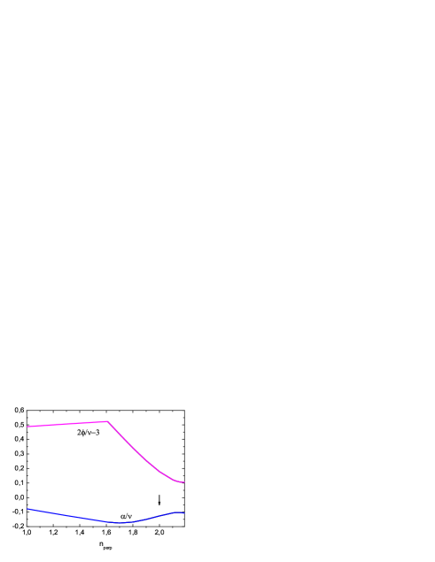
Figure 1: Exponents $\alpha/\nu$ and $2\phi/\nu-3$ appearing in Eqs. (84) and (86) at $n_{\|}=1$ as function of $n_{\perp}$. Note that via relation (117) $2\phi/\nu-3=z-2$ the strong dynamical scaling exponent $z$ results.

The explicit values of the above FPs depend on wether the isotropic Heisenberg or the biconical FP is inserted into the $\zeta$-functions. Eqs.(88)-(91) are valid up to two loop order. In three loop order it is known from the isotropic GLW-model that the function $B_{\phi^{2}}$ gets $u^{2}$-contributions changhoughton80 . In the multicritical GLW-model the matrix $\mbox{\boldmath$B$}_{\phi^{2}}$ may also be non diagonal, and then Eq.(87) does not hold in this simple form.

In the case of the isotropic Heisenberg FP $u_{\perp}^{\star}=u_{\|}^{\star}=u_{\times}^{\star}=u^{\star}$ Eqs.(88)-(91) simplify considerably. The ratios of the elements of the $\mbox{\boldmath$\zeta$}_{\phi^{2}}$-matrix reduce to

$$\frac{\big{[}\mbox{\boldmath$\zeta$}_{\phi^{2}}^{\star}\big{]}_{12}}{\zeta_{+}^{\star}-\big{[}\mbox{\boldmath$\zeta$}_{\phi^{2}}^{\star}\big{]}_{22}}=1=\frac{\gamma_{\|}^{\star}}{\gamma_{\perp}^{\star}}$$ (92)

for Case a and

$$\frac{\big{[}\mbox{\boldmath$\zeta$}_{\phi^{2}}^{\star}\big{]}_{21}}{\zeta_{-}^{\star}-\big{[}\mbox{\boldmath$\zeta$}_{\phi^{2}}^{\star}\big{]}_{11}}=-\frac{n_{\|}}{n_{\perp}}=\frac{\gamma_{\perp}^{\star}}{\gamma_{\|}^{\star}}\,,$$ (93)

for Case b. For the second equalities (83) and (85) have been used. Together with the relations $\varepsilon-2\zeta_{+}^{\star}=\alpha/\nu$ and $\varepsilon-2\zeta_{-}^{\star}=\phi/\nu-d$, which introduce the critical exponents and follow from Eqs. (80), (81) and (82) in paper I, the values for the isotropic Heisenberg FP are:
Case a: $\gamma_{+}^{\star}\neq 0$, $\gamma_{-}^{\star}=0$:

$$\gamma_{\perp}^{\star 2}=\gamma_{\|}^{\star 2}=\frac{2}{n_{\perp}+n_{\|}}\frac{\alpha}{\nu}\,.$$ (94)

Case b: $\gamma_{+}^{\star}=0$, $\gamma_{-}^{\star}\neq 0$:

$$\gamma_{\perp}^{\star 2}=\frac{2}{n_{\perp}+n_{\|}}\frac{n_{\|}}{n_{\perp}}\left(2\frac{\phi}{\nu}-d\right)\,,$$ (95)

$$\gamma_{\|}^{\star 2}=\frac{2}{n_{\perp}+n_{\|}}\frac{n_{\perp}}{n_{\|}}\left(2\frac{\phi}{\nu}-d\right)\,.$$ (96)

Note that due to the sign in Eq.(93) the relation

$$\gamma_{\|}^{\star}\gamma_{\perp}^{\star}=-\frac{2}{n_{\perp}+n_{\|}}\left(2\frac{\phi}{\nu}-d\right)$$ (97)

holds in this case. For $n_{\|}=1$ and $n_{\perp}=2$ our results agree with those of Ref.dohmmulti83 .

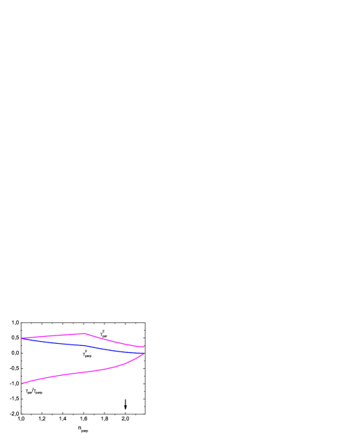
Figure 2: Fixed point values of the asymmetric static couplings $\gamma_{\|}$ and $\gamma_{\perp}$ for Case b ($\gamma_{\perp}^{\star}=0$, $\gamma_{\|}^{\star}\neq 0$) at the Heisenberg FP ($n_{\perp}<1.61$) and the biconical FP ($1.61<n_{\perp}<2.18$).

V.1.4 Resummation procedure

As in our former paperspartI ; partII of this series, in order to get numerical estimates we proceed within fixed dimension RG technique, i.e. we evaluate RG expansions in couplings $\{u_{\|},u_{\perp},u_{\times}\}$ at fixed $d=3$. Furthermore, as far as the expansions are known to have zero radius of convergence we use resummation techniqueresum to get reliable numerical estimates. The results given below were obtained within such a technique applied to the two-loop RG expansions. One of the ways to judge about typical numerical accuracy of our data, is to give an estimate for some cases where the expansions (and, subsequently, their numerical estimates) are known within much higher order of loops. As far as the static exponents $\alpha$ and $\nu$ explicitly enter many of formulas considered above, let us take them as an example. Namely, let us estimate relations

$$(2\phi/\nu-d)|_{d=3} \equiv 2/\nu_{-}-3,\,,$$ (98)

$$\alpha/\nu|_{d=3} \equiv 2/\nu_{+}-3\,,$$ (99)

that enter the formulas for the couplings $\gamma_{\perp}$, $\gamma_{\|}$. The exponents $\nu_{+}$ and $\nu_{-}$ have been defined in Eqs. (80) and (81) of paper I. Fig. 1 shows the dependence of $2\phi/\nu-3$ and of $\alpha/\nu$ on the order parameter component numbers $n_{\perp}$ at fixed $n_{\|}=1$. Recall that of main interest for us will be the physical case $n_{\|}=1$, $n_{\perp}=2$ indicated by the arrow. The region of $n_{\perp}$ shown in the figure covers also the region of stability of the Heisenberg $O(n)$-symmetrical FP, with $n=n_{\|}+n_{\perp}$. In particular it starts at $n_{\perp}=1$ near the marginal field dimension $n_{c}$ at which the exponent $\alpha$ changes its sign. For the $O(n)$ vector model an estimate based on the fixed $d=3$ six loop RG expansions reads Bervillier86 : $n_{c}=1.945\pm 0.002$. We get for the correlation length critical exponent in the Heisenberg $O(2)$ FP: $\nu=0.684$, via hyperscaling relation this leads to $\alpha=-0.053$. Our estimate correctly reproduces the absence of a divergency in the specific heat of $O(2)$ model ($\alpha$ is negative), however the value of $n_{c}\simeq 1.6$ we get is rather underestimated. Note however, that the fixed $d$ approach we exploit in two loop approximation is essentially better than the corresponding $\varepsilon$ expansion. Indeed, in two-loop $\varepsilon$-expansion one gets: $n_{c}=4-4\varepsilon$, which does not lead to reasonable estimates note1 . The two loop estimate of the massive field theory at $d=3$, $m_{c}\simeq 2.01$ Jug83 , is more close to the most accurate value of Ref.Bervillier86 , however it gives a wrong sign for the exponent $\alpha$. In any case the negative value of $\alpha$ for $n_{\perp}=2$ agrees with other calculations as reported in paper I.

It turns out (see below) that Case b is the stable FP for the asymmetric couplings. In order to evaluate numerically the values of couplings $\gamma_{\|}^{2}$, $\gamma_{\perp}^{2}$, we therefore substitute the resummed fixed point values of the static couplings $\{u_{\|},u_{\perp},u_{\times}\}$ into formulas (90), (91) and resum the resulting expression. In principle, one can use different ways for such an evaluation. Indeed, as we proceeded before, one can present these formulas in the form of expansion in renormalized couplings (keeping the two-loop terms) and resum the resulting second-order polynomial. Alternatively, based on the observation that numerator and denominator of Eqs. (90), (91) contain combinations of critical exponents, one can resum the numerator and the denominator separately. We will exploit both ways which naturally will lead to slightly different numerical estimates. This difference may also serve to get an idea about typical numerical accuracy of the results. Separately, we will evaluate the ratios $\gamma_{\perp}/\gamma_{\|}$. Again, it will be done by resummation of the series for this ratio, Eq. (85), as well as by using resummed values for $\gamma_{\|}^{2}$, $\gamma_{\perp}^{2}$.In particular, for $n_{\|}=1$, $n_{\perp}=2$ we get: $(\gamma_{\perp}^{\star})^{2}=0.034$, $(\gamma_{\|}\star)^{2}=0.286$ (when denominator and numerator are resummed separately), and $(\gamma_{\perp}^{\star})^{2}=0.031$, $(\gamma_{\|}\star)^{2}=0.293$ (when an entire expression is resummed). Resulting differences of the order of several percents bring about a typical numerical accuracy of the estimates. In Fig. 2 we plot the FP values of the asymmetric couplings and their ratio obtained within resummation of the entire expressions. These values will be used below to calculate the critical dynamics.

V.2 Static transient exponents

The stability of the fixed points is determined by the sign of the corresponding transient exponents. Latter can be found from the eigenvalues of the matrix

$$\frac{\partial\beta_{\gamma_{\alpha}}}{\partial\gamma_{\beta}}$$ (100)

with $\alpha,\beta=\perp,\|$. Inserting (IV.1) into (100) the corresponding eigenvalues read

$$\lambda^{(\pm)}=\frac{1}{2}\Bigg{\{}-\varepsilon+n_{\perp}\gamma_{\perp}^{2}+n_{\|}\gamma_{\|}^{2}+\big{[}\mbox{\boldmath$\zeta$}_{\phi^{2}}\big{]}_{11}+\big{[}\mbox{\boldmath$\zeta$}_{\phi^{2}}\big{]}_{22}$$

$$\pm\Bigg{[}\Bigg{(}\frac{n_{\perp}\gamma_{\perp}^{2}-n_{\|}\gamma_{\|}^{2}}{2}+\big{[}\mbox{\boldmath$\zeta$}_{\phi^{2}}\big{]}_{11}-\big{[}\mbox{\boldmath$\zeta$}_{\phi^{2}}\big{]}_{22}\Bigg{)}^{2}$$

$$+\big{(}n_{\perp}\gamma_{\perp}\gamma_{\|}+2\big{[}\mbox{\boldmath$\zeta$}_{\phi^{2}}\big{]}_{12}\big{)}\big{(}n_{\|}\gamma_{\perp}\gamma_{\|}+2\big{[}\mbox{\boldmath$\zeta$}_{\phi^{2}}\big{]}_{21}\big{)}\Bigg{]}^{1/2}\Bigg{\}}\,.$$ (101)

The above eigenvalues are valid in two loop order because Eq.(87) already has been used. The transient exponents

$$\omega_{\gamma}^{(\pm)}\equiv\lambda^{(\pm)}\Big{(}\{u\}=\{u^{\star}\},\{\gamma\}=\{\gamma^{\star}\}\Big{)}$$ (102)

are calculated by inserting the fixed point values of the static couplings into the eigenvalues. With the fixed point values (94) - (96) and Eq. (V.2) we obtain for the isotropic Heisenberg FP the transient exponents
Case a: $\gamma_{+}^{\star}\neq 0$, $\gamma_{-}^{\star}=0$:

$$\omega^{(+)}=\frac{\alpha}{\nu}\ ,\qquad\omega^{(-)}=-\bar{W}^{\star}\,.$$ (103)

Case b: $\gamma_{+}^{\star}=0$, $\gamma_{-}^{\star}\neq 0$:

$$\omega^{(+)}=2\frac{\phi}{\nu}-d\ ,\qquad\omega^{(-)}=\bar{W}^{\star}\,.$$ (104)

$\bar{W}^{\star}$ is the root

$$\bar{W}\equiv\sqrt{\Big{(}\big{[}\mbox{\boldmath$\zeta$}_{\phi^{2}}\big{]}_{11}-\big{[}\mbox{\boldmath$\zeta$}_{\phi^{2}}\big{]}_{22}\Big{)}^{2}+4\big{[}\mbox{\boldmath$\zeta$}_{\phi^{2}}\big{]}_{12}\big{[}\mbox{\boldmath$\zeta$}_{\phi^{2}}\big{]}_{21}}$$ (105)

taken at the fixed point values of the couplings. It is always positive and reads at the isotropic Heisenberg FP in two loop order

$$\bar{W}^{\star}=\frac{n_{\perp}+n_{\|}}{6}u^{\star}\left(1-\frac{u^{\star}}{3}\right)\,.$$ (106)

Thus one concludes that Case b is the stable FP even if $\alpha$ would be positiverem2 . For the biconical FP the stability of Case b can be verified explicitly by the flow of the couplings.

V.3 Dynamical fixed points

Calculations of the dynamical FPs values are done by solving the FP equations for the dynamical $\beta$-functions. Since only two of the equations (58)-(60) are independent the third equation serves as consistency check of the solution found. It is useful to choose for this purpose Eqs (59) and (60) for the time scale ratios $w_{\|}$ and $w_{\perp}$. Then one has to solve

$$\beta_{w_{\|}}(w_{\|},w_{\perp},w_{\|}/w_{\perp}) = 0\,,$$ (107)

$$\beta_{w_{\perp}}(w_{\|},w_{\perp},w_{\|}/w_{\perp}) = 0\,.$$

To find the dynamical FP values coordinates, the resummed FP values of static couplings $u_{\|}^{*},u_{\perp}^{*},u_{\times}^{*},\gamma_{\perp}^{*},\gamma_{\|}^{*}$ are inserted into these equationsnote2 .

The dynamical FPs depend on which static FP is considered. There might be several dynamical FPs for one static FP, which could be either strong dynamical or weak dynamical scaling FPs. Since also unstable static FPs might be reached in the asymptotics if one starts with static initial conditions in the attraction region of this FP (a subspace in the space the static couplings see e.g. Fig. 3 in paper I) at least both the Heisenberg FP and the biconical FP have to be taken into consideration. It turns out that in both cases apart from the trivial unstable FP where all timescale ratios are zero (see below) two dynamical FPs are found: (i) an unstable weak dynamical scaling FP corresponding to model A and (ii) a stable new strong dynamical scaling FP. In the physical interesting case $n_{\|}=1$ and $n_{\perp}=2$ these cases correspond to dynamical behavior at a multicritical point of bicritical and tetracritical type respectively. The different types of weak and strong dynamical FPs are shown in Tab. 2.

FP	scaling type	$v$	$w_{\|}$	$w_{\perp}=w_{\|}/v$	$z_{\phi_{\|}}$	$z_{\phi_{\perp}}$	$z_{m}$
$\mathcal{H}_{C_{w}}$	weak	0	$w_{\|{C_{w}}}^{\mathcal{H}}$	$\infty$	$2\frac{\phi}{\nu}-1$	infinite fast	$2\frac{\phi}{\nu}-1$
$\mathcal{H}_{A}$	weak	$v_{A}^{({\mathcal{H}})}$	0	0	$2+c\eta$	$2+c\eta$	$2\frac{\phi}{\nu}-1$
$\mathcal{H}_{C}$	strong	$v_{C}^{\mathcal{H}}$	$w^{\mathcal{H}}_{\|}$	$w^{\mathcal{H}}_{\perp}$	$2\frac{\phi}{\nu}-1$	$2\frac{\phi}{\nu}-1$	$2\frac{\phi}{\nu}-1$
$\mathcal{B}_{C_{w}}$	weak	0	$w_{\|{C_{w}}}^{\mathcal{B}}$	$\infty$	$2\frac{\phi}{\nu}-1$	infinite fast	$2\frac{\phi}{\nu}-1$
$\mathcal{B}_{A}$	weak	$v_{A}^{({\mathcal{B}})}$	$0$	$0$	$z^{\mathcal{B}}$	$z^{\mathcal{B}}$	$2\frac{\phi}{\nu}-1$
$\mathcal{B}_{C}$	strong	$v_{C}^{({\mathcal{B}})}$	$w^{\mathcal{B}}_{\|}$	$w^{\mathcal{B}}_{\perp}$	$2\frac{\phi}{\nu}-1$	$2\frac{\phi}{\nu}-1$	$2\frac{\phi}{\nu}-1$

Table 2: Types of dynamical FPs for the static Heisenberg and biconical FP. Not included is the trivial unstable fixed point with all times scale ratios equal to zero. The value of $c$ reads $c=6\ln(4/3)-1$. Note that for the weak scaling FP the result is only valid in two loop order, whereas the relation of the dynamical critical exponent in the strong scaling FP holds in all orders.

V.3.1 Strong dynamical scaling fixed point

FP	$u_{\|}^{\star}$	$u_{\perp}^{\star}$	$u_{\times}^{\star}$	$\gamma_{\|}^{\star 2}$	$\gamma_{\perp}^{\star 2}$	$v^{\star}$	$w_{\perp}^{\star}$	$w_{\|}^{\star}$
${\mathcal{B}_{C}}$, a	1.28745	1.12769	0.30129	0.29378	0.03170	$6.09592\cdot 10^{-43}$	$1.24285\cdot 10^{42}$	0.75763
${\mathcal{H}_{C}}$, b						7.29393$\cdot 10^{-5}$	1.55665$\cdot 10^{4}$	1.13541
${\mathcal{H}_{C}}$, a	$1.00156$	$1.00156$	$1.00156$	$0.72554$	$0.18139$	7.30771$\cdot 10^{-5}$	1.55372$\cdot 10^{4}$	1.13541

Table 3: FP values of couplings and timescale ratios for $n_{\|}=1$, $n_{\perp}=2$. a FP values of the timescale ratios found via approximation using Eqs. (100), (101), as described in the text with the values for FP ${\mathcal{B}}$: $A=0.09770$, $B=0.00101$ and the FP ${\mathcal{H}}$: $A=0.31534$, $B=0.03311$. b numerical solution for the FP values of the timescale ratios;

In order to find the strong dynamical scaling FPs it is not necessary to discriminate between the static Heisenberg FP or the biconical FP although the dynamical equations to be solved simplify in the first case a little bit. Thus we use the results for the FP values derived in paper I for the quartic couplings $\{u\}$ and the FP values for the asymmetric couplings $\{\gamma\}$ of Case b (see Eqs. (85), (90) and (91)). At the strong scaling dynamical FP all timescale ratios have to be nonzero and finite. Moreover due to the definitions of the timescale ratios it follows that $w_{\|}^{\star}=v^{\star}w_{\perp}^{\star}$. This dynamical strong scaling FP value is found by setting the differences of two of the three dynamical $\zeta$-functions, (49)-(IV.2) to zero leading to three equations. Since there are only two independent time ratios the third equation can be used to check the results.

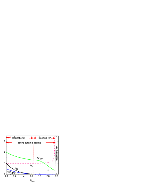
Figure 3: Fixed point values of the timescale ratios $v$, $1/w_{\perp}$ and $w_{\|}$ for the static stable FPs: the isotropic Heisenberg FP ($n_{\perp}<1.61$) and the biconical FP ($1.61<n_{\perp}<2.18$). Strong dynamical scaling is valid up to the stability borderline to the decoupling FP. In the biconical region the values of $v_{C}$ and $1/w_{C\perp}$ are finite but not to distinguish from zero on this scale. The notation of the dynamical FPs correspond to the notation in Tab 2. The dashed curve shows the unstable model A FP (see text).

The FP values (FP with subscript $C$ in Tab. 2) have been plotted in Fig. 3 for different $n_{\perp}$ at $n_{\|}=1$ and the numerical values for $n_{\perp}=2$ are collected in Tab. 3. This shows that the FP value of the timescale ratio for $v$ is different from the FP value found in the pure relaxational model A. These were at the Heisenberg FP $v^{\star}_{A}=1$ and at the biconical FP $v^{\star}=v^{\mathcal{B}}_{A}$ with $v^{\mathcal{B}}_{A}\to\infty$ in approaching the stability borderline to the decoupling fixed point (see Fig. 1 in paper II).

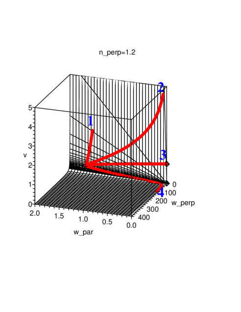
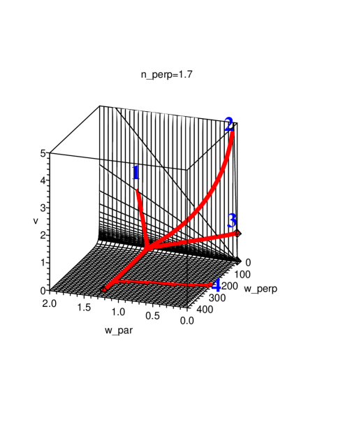
Figure 4: Dynamical flow at $n_{\|}=1$ and different $n_{\perp}$ values for different dynamical initial conditions numbered 1 to 4. The static couplings are chosen to be fixed at their stable FP values (the isotropic Heisenberg FP for $n_{\perp}=1.2$, the biconical FP for $n_{\perp}=1.7$). The dynamical FP values are $v^{\star}=0.399$, $0.004$, $w^{\star}_{\|}=1.661$, $1.300$ and $w^{\star}_{\perp}=4.159$, $351.06$ at ${\cal H_{C}}$, ${\cal B_{C}}$ respectively. Also shown is the surface $v=w_{\|}/w_{\perp}$ to which the flow is restricted.

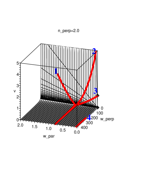
Figure 5: Dynamical flow at $n_{\|}=1$ and $n_{\perp}=2$ for different dynamical initial conditions numbered 1 to 4. The static couplings are chosen to be fixed at their biconical FP values. The static and dynamical FP values of ${\cal B_{C}}$ are given in Tab. 3. The dynamical FP lies outside the region shown. Also shown is the surface $v=w_{\|}/w_{\perp}$ to which the flow is restricted.

A numerical problem arises in finding the FP values of $v$ and $1/w_{\perp}$when they reach very small values. It cannot be numerically decided wether the FP values are zero or finite. In order to clarify the existence or nonexistence of a weak scaling FP one has to look for an analytic expression for the small FP values. However it is numerically easy to find the FP value of $w_{\|}$ which is nonzero and finite in the whole region up to the stability borderline between the biconical and decoupling FP. In order to solve this problem the dependence of the $\zeta$-functions are studied within this region. One observes that there are logarithmic terms which would diverge in the limit $v\to 0$ under the condition $w_{\perp}=w_{\|}/v$. Thus one obtains two equations for the FP value of $v$ and $w_{\|}$. In the equation for the FP of $w_{\|}$ one might safely perform the limit $v\to 0$ and $w_{\perp}\to\infty$. This leads to

$$0=\zeta_{\Gamma_{\|}}^{(C)}\big{(}\{u^{\star}\},\{\gamma^{\star}\},v=0,w_{\|},w_{\perp}\to\infty\big{)}-2\zeta^{\star}_{m}\,.$$ (108)

Using limiting functions

$$\zeta_{\Gamma_{\|}}^{(A)}=\frac{n_{\|}+2}{36}\ u_{\|}^{\star 2}\left(3\ln\frac{4}{3}-\frac{1}{2}\right)-\frac{n_{\perp}}{72}\ u_{\times}^{\star 2}$$ (109)

and

$$\zeta_{\Gamma_{\|}}^{(C_{\|})}\big{(}u^{\star}_{\|},\gamma^{\star}_{\|},w_{|}\big{)}=\frac{w_{\|}\gamma_{\|}^{\star 2}}{1+w_{\|}}\Bigg{\{}1-\frac{1}{2}\Bigg{[}\frac{n_{\|}+2}{3}$$

$$u^{\star}_{\|}\Big{(}1-3\ln\frac{4}{3}\Big{)}+\frac{w_{\|}\gamma_{\|}^{\star 2}}{1+w_{\|}}\Bigg{(}\frac{n_{\|}}{2}-\frac{w_{\|}}{1+w_{|}}-$$ (110)

$$\frac{3(n_{\|}+2)}{2}\ln\frac{4}{3}-\frac{(1+2w_{\|})}{1+w_{\|}}\ln\frac{(1+w_{\|})^{2}}{1+2w_{\|}}\Bigg{)}\Bigg{]}\Bigg{\}}$$

then Eq. (108) reads

$$0=\frac{w_{\|}\gamma_{\|}^{\star 2}}{1+w_{\|}}\Bigg{\{}1-\frac{1}{2}\Bigg{[}\frac{n_{\|}+2}{3}u^{\star}_{\|}\Big{(}1-3\ln\frac{4}{3}\Big{)}$$

$$+\frac{w_{\|}\gamma_{\|}^{\star 2}}{1+w_{\|}}\Bigg{(}\frac{n_{\|}}{2}-\frac{w_{\|}}{1+w_{\|}}-\frac{3(n_{\|}+2)}{2}\ln\frac{4}{3}$$

$$-\frac{1+2w_{\|}}{1+w_{\|}}\ln\frac{(1+w_{\|})^{2}}{1+2w_{\|}}\Bigg{)}\Bigg{]}\Bigg{\}}$$ (111)

$$-\frac{n_{\perp}}{4}\frac{w_{\|}\gamma^{\star}_{\|}\gamma^{\star}_{\perp}}{1+w_{\|}}\Bigg{[}\frac{2}{3}u_{\times}+\frac{w_{\|}\gamma^{\star}_{\|}\gamma^{\star}_{\perp}}{1+w_{\|}}\Bigg{]}$$

$$+\frac{n_{\|}+2}{36}\ u_{\|}^{\star 2}\left(3\ln\frac{4}{3}-\frac{1}{2}\right)-\frac{n_{\perp}}{72}\ u_{\times}^{\star 2}-2\zeta^{\star}_{m}$$

This equation is solved numerically to give the value of $w_{\|}^{\star}$ which then is inserted into the second equation for $v^{\star}$. In order to find $v^{\star}$ one collects the logarithmic diverging terms in the equation for $v^{\star}$,

$$\zeta_{\Gamma_{\|}}^{(C)}(v,w_{\|},w_{\|}/v)-\zeta_{\Gamma_{\perp}}^{(C)}(v,w_{\|},w_{\|}/v)=0\,.$$ (112)

In the remaining terms the limit $v\to 0$ can safely performed. Then the solution reads

$$\ln v^{\star}=-\frac{A}{B}$$ (113)

with

$$A=2\zeta^{\star}_{m}-\gamma_{\perp}^{\star 2}\Bigg{\{}1-\frac{1}{2}\Bigg{[}\frac{n_{\perp}+2}{3}u^{\star}_{\perp}\Big{(}1-3\ln\frac{4}{3}\Big{)}$$

$$+\gamma_{\perp}^{\star 2}\Bigg{(}\frac{n_{\perp}}{2}-1-\frac{3(n_{\perp}+2)}{2}\ln\frac{4}{3}-2\ln\frac{w^{\star}_{\|}}{2}\Bigg{)}\Bigg{]}\Bigg{\}}$$

$$+\frac{n_{\|}}{4}\gamma^{\star}_{\perp}\gamma^{\star}_{\|}\Bigg{[}\frac{2}{3}u^{\star}_{\times}+\gamma^{\star}_{\perp}\gamma^{\star}_{\|}\Bigg{]}\ln 2-\frac{n_{\perp}+2}{36}\ u_{\perp}^{\star 2}$$

$$\left(3\ln\frac{4}{3}-\frac{1}{2}\right)-\frac{n_{\|}}{72}\ u_{\times}^{\star 2}\Big{(}1-2\ln 2\Big{)}$$ (114)

and

$$B=\gamma_{\perp}^{\star 4}+\frac{n_{\|}}{36}u_{\times}^{\star 2}+\frac{n_{\|}}{4}\gamma^{\star}_{\perp}\gamma^{\star}_{\|}\Bigg{[}\frac{2}{3}u^{\star}_{\times}+\gamma^{\star}_{\perp}\gamma^{\star}_{\|}\Bigg{]}\,.$$ (115)

It can be shown that $A$ and $B$ are positive. Approaching the stability borderline to the decoupling FP $A$ stays finite and $B$ goes to zero since $u^{\star}_{\times}$ and $\gamma^{\star}_{\perp}$ go to zero. In consequence $v^{\star}$ goes to zero and $w^{\star}_{\perp}$ goes to infinity in and only in this limit. The analytic solution found within this region joins smoothly to the numerical solution found for larger values of the timescale ratios. Thus it is proven that in the whole region where the Heisenberg FP or the biconical FP is stable dynamical strong scaling holds.

Considering the FP values for the timescale ratios for the Heisenberg FP in the region of $n_{\perp}>1.7$ (where it is reached only for static initial conditions in a subspace of the fourth order couplings) one also finds a small value for $v^{\star}$, a very large value for $w_{\perp}^{\star}$ and a nonzero finite value for $w_{\|}^{\star}$. However contrary to the biconical FP now $A$ and $B$ stay finite at the stability borderline between the biconical FP and the decoupling FP at $n_{\perp}\sim 2.18$. Indeed the values calculated for the Heisenberg FP from Eqs (V.3.1) and (115) are $A=0.34866$, $B=0.02558$ whereas for the biconical FP one obtains $A=0.05268$, $B=4.27958\cdot 10^{-9}$.

The asymptotic dynamical exponents are obtained from the values of the $\zeta$-functions at the FP:

$$z_{\phi_{\|}}=2+\zeta^{\star}_{\Gamma_{\|}}\qquad z_{\phi_{\perp}}=2+\zeta^{\star}_{\Gamma_{\perp}}\qquad z^{\star}_{m}=2+\zeta_{\lambda}\,.$$ (116)

At the strong dynamical scaling FP all dynamical $\zeta$-functions are equal to twice the static $\zeta$-function $\zeta_{m}$. Therefore the CD induces the value of the dynamical critical exponent $z$

$$z=2+2\zeta_{m}^{\star}=2\frac{\phi}{\nu}-1$$ (117)

according to Eq. (44) and Eq. (86). The values for the static exponents depend on which static FP is stable. For $n_{\|}=1$ the $n_{\perp}$-dependence of $z-2$ is shown in Fig. 1.

V.3.2 Weak dynamical scaling fixed point

Weak dynamical scaling FPs are solutions of the dynamical FP equations where one or more of the FP values of the timescale ratios are zero or infinite. Such a weak dynamical scaling FP has already been found in model A and it became stable at the stability borderline to the decoupling FP.

Indeed Eqs (107) allow solutions where both timescale ratios $w_{\|}$ and $w_{\perp}$ are zero. In such a case one has to rely on the third equation for the ratio $v=w_{\|}/w_{\perp}$ to find the limiting FP value. However in the limit $w_{\|}\to 0$ and $w_{\perp}\to 0$ Eq. (58) for $v$ reduces to the FP equation of model A (FP with subscript $A$ in Tab. 2). Thus one recovers the model A FPs in this case.

There is no solution $w^{\star}_{\|}=v^{\star}=0$ and $w_{\perp}$ nonzero and finite due to the $\ln v$ term in (IV.2). For a similar reason no FP with $w^{\star}_{\|}$ nonzero and finite, $w^{\star}_{\perp}=0$ and $v^{\star}=\infty$ is possible. However a FP with $w^{\star}_{\|}$ nonzero and finite, $v^{\star}=0$ and $w_{\perp}=\infty$ is possible (FP with subscript $C_{w}$ in Tab. 2). The values of $w_{\|}^{\star}$ are obtained from Eq. (V.3.1), but now these values are not an approximation but the exact $C_{w}$ FP values for any $n_{\|}$ and $n_{\perp}$.

The dynamical critical exponents may be different in the case of weak dynamical scaling. For the weak model C FP (subscript ${C_{w}}$) $w_{\|}^{\star}$ is finite and nonzero therefore $\zeta_{\Gamma_{\|}}^{\star}=\zeta_{\lambda}^{\star}$ and $z_{\phi_{\|}}=2\frac{\phi}{\nu}-1$. Thus the CD sets the timescale for the OP $\phi_{\|}$. Inserting $w_{\perp}^{\star}=\infty$ into $\zeta_{\Gamma_{\perp}}$ leads due to logarithmic diverging terms to an infinite value of the corresponding dynamical exponent $z_{\phi_{\perp}}$. This indicates that the density $\phi_{\perp}$ is much faster than the other densities. It is especially much faster than the other OP $\phi_{\|}$.

In the case where both FP values of the timescale ratios $w_{\|}$ and $w_{\perp}$ are zero and $v$ is finite and nonzero, both OPs have the same timescale with the dynamical exponent (of model A) $z=2+c\eta$ different from the exponent of the CD $z_{m}=2\frac{\phi}{\nu}-1$.

V.4 Dynamical transient exponents

The dynamical transient exponents can be calculated from the matrix of the derivatives of the $\beta$-function with respect to the timescale ratios $v$, $w_{\|}$ and $w_{\perp}$. Since only two timescale ratios are independent only two are considered in the stability matrix. The eigenvalues of the $2\times 2$-matrix have to be positive for the overall stable FP otherwise the FP is unstable. In the following the timescale ratios $w_{\|}$ and $w_{\perp}$ are chosen as independent.

The model A type FP with $v^{\star}=v_{A}$ nonzero and finite is unstable since the two eigenvalues,

$$\omega_{w_{\|}}=\zeta^{\star}_{\Gamma_{\|}}-2\zeta^{\star}_{m}\qquad\mbox{and}\qquad\omega_{w_{\perp}}=\zeta^{\star}_{\Gamma_{\perp}}-2\zeta^{\star}_{m}$$ (118)

are negative. In fact they are equal because $\zeta^{\star}_{\Gamma_{\|}}=\zeta^{\star}_{\Gamma_{\perp}}$. Their values are calculated with $2\zeta^{\star}_{m}=2\phi/\nu-1$ and inserting the model A FP value $v^{\star}=v_{A}$ (see Fig 3) and $w_{\|}^{\star}=w_{\perp}^{\star}=0$. Then $\zeta^{\star}_{\Gamma_{\|}}-2\phi/\nu+1<0$ and $\omega_{w_{\|}}=-0.126$ for $n_{\|}=1$ and $n_{\|}=2$.

Similarly the instability of the FP with $v^{\star}=w_{\|}^{\star}=w_{\perp}^{\star}=0$ can be shown. However some care has to be taken due to the vanishing timescale ratio $v$. The eigenvalues are again given by Eq. (118) but now they are different. Whereas $\omega_{w_{\|}}$ is negative $\omega_{w_{\perp}}$ goes to $\infty$ due to the $\ln v$ term in the model A $\zeta$ function (IV.2).

The transient exponent for the strong scaling FP are the eigenvalues of the matrix of derivatives of the $\beta$-functions according to the timescale ratios at the FP

$$\left(\begin{array}[]{cc}\frac{\partial\beta_{w_{\|}}}{\partial w_{\|}}&\frac{\partial\beta_{w_{\|}}}{\partial w_{\perp}}\\ \frac{\partial\beta_{w_{\perp}}}{\partial w_{\|}}&\frac{\partial\beta_{w_{\perp}}}{\partial w_{\perp}}\end{array}\right)^{\star}=\left(\begin{array}[]{cc}w_{\|}\left(\frac{\partial\zeta_{\Gamma_{\|}}}{\partial w_{\|}}\right)&w_{\|}\left(\frac{\partial\zeta_{\Gamma_{\|}}}{\partial w_{\perp}}\right)\\ w_{\perp}\left(\frac{\partial\zeta_{\Gamma_{\perp}}}{\partial w_{\|}}\right)&w_{\perp}\left(\frac{\partial\zeta_{\Gamma_{\perp}}}{\partial w_{\perp}}\right)\end{array}\right)^{\star}\,.\\$$ (119)

Use has been made from the independence of $\zeta_{\lambda}$ on the timescale ratios. The nondiagonal elements depend on the timescale ratios by which they are derived only via $v$ and therefore are proportional to $1/w_{\perp}$. In the region where $w_{\perp}$ is very large the two eigenvalues are then given by the diagonal elements.

$$\omega_{w\|}=w_{\|}^{\star}\left(\frac{\partial\zeta_{\Gamma_{\|}}}{\partial w_{\|}}\right)^{\star}\,,\quad\omega_{w_{\perp}}=w_{\perp}^{\star}\left(\frac{\partial\zeta_{\Gamma_{\perp}}}{\partial w_{\perp}}\right)^{\star}\,.$$ (120)

Near the stability borderline to the decoupling FP the second eigenvalue goes to zero according to

$$\omega_{w_{\perp}}=B+{\cal O}(1/w_{\perp})$$ (121)

with $B$ from Eq. (115), being exactly zero at the borderline. The value of the slow transient at $n_{\|}=1$ and $n_{\perp}=2$ is given by $\omega_{w_{\perp}}=0.001$ Thus as shown in the next section in this case nonasymptotic effects are present in the physical accessible region.

As already mentioned for the Heisenberg FP ${\cal H_{C}}$ $B$ does not reach zero at the borderline but its value is one order smaller than the static transient exponents. At $n_{\perp}=2$ and $n_{\perp}=2.18$ the value of the dynamical transient exponent is given by $\omega_{w_{\perp}}=0.033$ and $\omega_{w_{\perp}}=0.026$ respectively.

VI Dynamical flows and effective exponents

The flow of the timescale ratios is described by the RG equations

$$l\frac{\partial v}{\partial l} = \beta_{v}(\{u\},\{\gamma\},\{w\})\,,$$

$$l\frac{\partial w_{\perp}}{\partial l} = \beta_{w_{\perp}}(\{u\},\{\gamma\},\{w\})\,,$$ (122)

$$l\frac{\partial w_{\|}}{\partial l} = \beta_{w_{\|}}(\{u\},\{\gamma\},\{w\})\,,$$

with the $\beta$-functions Eqs. (58)-(59). Note, that the dynamical $\beta$-functions depend also on the RG equations of the static quartic couplings (Eqs (33)-(36) of paper I) and the RG equations of the asymmetric couplings

$$l\frac{\partial\vec{\gamma}}{\partial l}=\vec{\beta}_{\gamma}(\{u\},\{\gamma\})$$ (123)

with the $\beta$-function Eq. (IV.1).

In order to simplify the picture it is assumed that the static couplings have already reached the FP by which they are attracted from their initial conditions. Then the RG flows are displayed in the three-dimensional space of the time-scale ratios $w_{\|},w_{\perp},v$ in Figs. 4 and 5 for the physical interesting case at $n_{\|}=1$, $n_{\perp}=2$. The static biconical FP is stable for this case in general. However for initial conditions on the surface separating the stable biconical FP from the Heisenberg FP the flow is attracted to the Heisenberg FP. Therefore one may also fix the static parameters to this FP.

To give an overview of the different patterns of the flows three different value of $n_{\perp}$ are chosen for fixed $n_{\|}=1$: (i) $n_{\perp}=1.2$, where the static Heisenberg FP is stable (Fig. 4), (ii) $n_{\perp}=1.7$ (Fig. 4) and (iii) $n_{\perp}=2$ (Fig. 5) where the biconical FP is stable.

In all cases the FP values of the timescales are nonzero and finite but the values of $v^{\star}$ becomes very small and $w_{\perp}^{\star}$ very large. The asymptotic approach to the FP in cases (ii) and (iii) occurs in the direction of the $w_{\perp}$-axis almost at $v\sim 0$ and $w_{|}\sim w^{\star}_{\|}$.

VI.1 Effective exponents

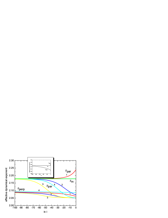
Figure 6: Effective dynamical exponents $z_{\|}$, $z_{\perp}$, and $z_{m}$ calculated along the different RG flows of Fig. 5 (indicated by the numbers). The insert shows that even for flow parameters as small as $\ln l=-2000$ the effective exponent $z_{\perp}$ has not reached its asymptotic value $2.18$.

We define the effective exponents by:

$$z_{\|\,eff}(l) = 2+\zeta_{\Gamma_{\|}}(\{u(l)\},\{\gamma(l)\},\{w(l)\}),$$

$$z_{\perp\,eff}(l) = 2+\zeta_{\Gamma_{\perp}}(\{u(l)\},\{\gamma(l)\},\{w(l)\}),$$

$$z_{m\,eff}(l) = 2+\zeta_{\lambda}(\{u(l)\})\,.$$ (124)

These exponents appear e.g. in the critical temperature and/or wave vector dependence of the transport coefficients describing the relaxation of the alternating magnetization or the diffusion of the magnetization in the direction of the external magnetic field. They are in principle experimentally accessible. An interesting feature is the independence of the effective dynamical scaling exponent $z_{m}$ of the CD from the dynamical timescales. Therefore its nonasymptotic value is only due to nonasymptotic effects within statics. This allows to trace back nonasymptotic effects in dynamical quantities to the slow transients in statics or those appearing in dynamics.

In order to calculate the numerical values of the effective exponents, we substitute into Eq. (124) the resummed coordinates of the static FP $\{u_{\|}^{*},u_{\perp}^{*},u_{\times}^{*}\}$ and the values of timescale ratios $\{w_{\|}(\ell),w_{\perp}(\ell),v(\ell)\}$ along the RG flow. Choosing the FP values of the static couplings fixes the asymptotic values of the effective dynamical exponents since they are expressed by the static asymptotic exponents for the strong dynamical scaling FP.

The results shown in Fig. 6 correspond to the case $n_{\|}=1$, $n_{\perp}=2$. We evaluate the timescale ratios along the previously obtained flows 1-4 in Fig. 5. The effective exponents for the different initial conditions are shown by numbered solid lines, As one can observe from this figure, the exponents calculated along several flows do not coincide for the values of the flow parameter shown. However one sees the merging of the different values for $z_{\|}$ to their asymptotic value $z_{\perp}^{\star}=z_{m}^{\star}=2.18$ given by the static value corresponding to the CD (the constant line in Fig. 6). More remarkable is the difference between the effective exponents for the parallel and perpendicular components of the OP. This difference can be traced back to the fact that $w_{\perp}$ did not reach its very large FP value due to the slow dynamical transient. Only for flow parameter values larger than $\ln l\sim-2000$ the effective exponent attains its asymptotic value $z_{\perp}\sim 2.18$ as it should be (see the insert of Fig. 6 where the smallest value is $\ln l=-2000$ for the flow 1).

Furthermore, we see that the exponent $z_{\|}$ flows towards its asymptotic value $z_{\|}=2.18$. In fact, exponent $z_{\perp}$ attains the asymptotic value $z_{\perp}=2.18$ as well, but for much smaller values of the flow parameter. In the insert of Fig. 6 we show this exponent for all flows within larger range of $\ln\ell$.

For certain initial values of the static parameters it is possible that the unstable Heisenberg FP is reached (see Fig. 3 in paper I the flow number 1, which lies on the surface separating the attraction region of the biconical FP from the flow away solutions. In such a case the effective exponents reach faster the asymptotic value of the dynamical exponent $z=2.44$ since the dynamical transient exponent $\omega_{w_{\perp}}=B$ is lager by a factor of $33$ (for the values of B see caption to Tab. 3).

VII Conclusion and outlook

The effect of coupling the conserved magnetization parallel to the external magnetic field to the two OPs (the components of the alternating magnetization parallel and perpendicular to the external magnetic field) leads to strong scaling dynamical behavior. This means that the timescales of all dynamical quantities scale with the same dynamical critical exponent $z=2\phi/\nu-2$. However this scaling behavior might be hidden by nonasymtotic effects dominating the physical accessible region when approaching the multicritical point due to a very small dynamical transient. This applies in the physical interesting case $n_{\|}=1$ and $n_{\perp}=2$ where one of the timescales is almost zero and the other one almost infinite. In consequence the magnetic transport coefficients might show different effective behavior with temperature when approaching the multicritical point. The dynamical amplitude ratios might be far from their asymptotic values and show nonuniversal behavior.

For a complete description in the whole $n_{\|}$-$n_{\perp}$-space the model presented here has to be extended in two ways. First for the physical case $n_{\|}=1$ and $n_{\perp}=2$ one has to introduce reversible terms in the equations of motions. Second one has to allow for an asymmetric coupling to a energy like CD in addition to the magnetization.

Acknowledgement: This work was supported by the Fonds zur Förderung der wissenschaftlichen Forschung under Project No. P19583-N20.

References

- (1) R. Folk, Y. Holovatch, and G. Moser, Phys. Rev. E 78, 041125 (2008); arXiv:0808.0314; henceforth called paper I
- (2) R. Folk, Y. Holovatch, and G. Moser, Phys. Rev.E 78, 041124 (2008); arXiv:0809.3146; henceforth called paper II
- (3) V. Dohm and H.-K. Janssen, Phys. Rev. Lett. 39, 946 (1977); J. Appl. Phys. 49, 1347 (1978)
- (4) Since at the multicritical point two different types of fluctuation are present corresponding to the two OPs there are also two types of slow conserved densities: (i) magnetic like and (ii) energy like. They correspond to the two fields: (i) the magnetic field and (ii) the temperature.
- (5) V. Dohm, Report of the Kernforschungsanlage Jülich Nr. 1578 (1979)
- (6) V. Dohm in Multicritical Phenomena, ed. Plenum, New York and London 1983 page 81
- (7) B. I. Halperin, P.C.Hohenberg, and Shang-keng Ma, Phys. Rev. B 10, 139 (1974); E. Brezin and C. De Dominicis, Phys. Rev. B 12, 4954 (1975)
- (8) R. Folk and G. Moser, Phys. Rev. Lett. 91, 030601 (2003)
- (9) D. R. Nelson, J. M. Kosterlitz, and M. E. Fisher, Phys. Rev. Lett. 33, 813 (1974); Y. Imry, J. Phys. C: Solid State Phys. 8, 567 (1975); I. F. Lyuksyutov, V. L. Pokrovskii, and D. E. Khmelnitskii, Sov. Phys. JETP 42, 923 (1975); V. V. Prudnikov, P. V. Prudnikov, and A. A. Fedorenko, JETP Lett. 68, 950 (1998); P. Calabrese, A. Pelissetto, and E. Vicari, Phys. Rev. 67, 054505 (2003)
- (10) V. Dohm, Z. Phys. B 60, 61 (1985); R. Schloms and V. Dohm, Europhys. Lett., 3, 413 (1987); R. Schloms and V. Dohm, Nucl. Phys. B 328, 639 (1989).
- (11) R. Folk and G. Moser, J. Phys. A: Math. Gen. 39, R207 (2006)
- (12) R. Folk and G. Moser, Phys. Rev. E 69, 036101 (2004).
- (13) M-C. Chang and A. Houghton, Phys. Rev. B 21, 1881 (1980)
- (14) We use the Padé-Borel resummation technique, as explained in details in paper I. For an overview see e.g. Yu. Holovatch, V. Blavats’ka, M. Dudka, C. von Ferber, R. Folk, and T. Yavors’kii, Int. J. Mod. Phys. B 16, 4027 (2002).
- (15) C. Bervillier, Phys. Rev. B 34, 8141 (1986).
- (16) For estimates of the marginal dimension see: M. Dudka, Yu. Holovatch, and T. Yavors’kii, Acta Phys. Slovaca 52, 323 (2002).
- (17) G. Jug, Phys. Rev. B 27, 609 (1983).
- (18) Two cautions are to be made at this point. First, due to the special structure of the dynamical vertex functions, the dynamical -functions contain only even powers of couplings and . Therefore, to define a sign of the coupling, one should use an additional condition, Eq. (85). Second, as far as the formulas for the dynamical -functions are non-polynomial, one can not use familiar resummation techniques for further numerical estimates. However one improves their convergence in an indirect way, by using there the resummed values for the static couplings.
- (19) Note that in Eq. (II.1) only one CD has been taken into account. In the most general case and especially when the specific heat is diverging one should allow for a second CD and four asymmetric couplings.