Fixation times in evolutionary games under weak selection
Abstract
In evolutionary game dynamics, reproductive success increases with the performance in an evolutionary game. If strategy performs better than strategy , strategy will spread in the population. Under stochastic dynamics, a single mutant will sooner or later take over the entire population or go extinct. We analyze the mean exit times (or average fixation times) associated with this process. We show analytically that these times depend on the payoff matrix of the game in an amazingly simple way under weak selection, i. e. strong stochasticity: The payoff difference is a linear function of the number of individuals , . The unconditional mean exit time depends only on the constant term . Given that a single mutant takes over the population, the corresponding conditional mean exit time depends only on the density dependent term . We demonstrate this finding for two commonly applied microscopic evolutionary processes.
1 Introduction
Systems in which successful strategies spread by imitation or genetic reproduction can be described by evolutionary game theory. Such models are routinely analyzed in evolutionary biology, sociology, anthropology and economics. Recently, the application of methods from statistical physics to these systems has lead to many important insights [1, 2, 3, 4, 5].
Traditionally, the dynamics is described by the replicator equations, where the growth rate of a strategy is associated with its relative success compared with the population average [6, 7].
In the past years, research has focused on stochastic evolutionary game dynamics in finite populations [8, 9, 10, 11, 12, 13, 14, 15, 16, 17, 18, 19, 20, 21, 22]. In this context, a connection to the weak selection limit of population genetics has been established [8]. Weak selection means that the payoff differences based on different strategic behavior in interactions represent only a small correction to otherwise random dynamics, similar to high temperature expansions in physics. Weak selection is considered as a relevant limit in biology, as most evolutionary changes are driven by small fitness differences [23]. Moreover, it allows analytical approximations that are often impossible when selective differences in payoffs are large [8, 24, 25].
Most of the recent work that uses the weak selection approximation has been focusing on the probability that a certain strategy takes over. The time associated with this process has been calculated [26], but it received considerably less attention so far. Here, we present the weak selection corrections to the conditional and unconditional mean exit or fixation times in evolutionary games with players.
The conditional average time to fixation is the expected time a single mutant needs to take over the population, given that such a takeover occurs at all. The unconditional average time of fixation is the expectation value for the time until the population is homogenous again after the arrival of a single mutant. This is regardless of wether the mutant type takes over the population or becomes extinct. Equivalently, the average fixation times for such one dimensional random walks can also be interpreted as mean first passage times or mean exit times [27, 28, 29].
Throughout this paper, we use the payoff matrix
| (1) |
An player interacting with another receives . If it interacts with , it obtains . Similarly, receives from and from other ’s. Thus, the average payoffs are
| (2) | |||||
| (3) |
A quantity that is of particular interest is the difference between the average payoffs,
| (4) |
where
| (5) | |||||
| (6) |
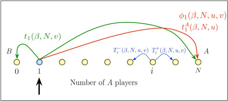
We show that under weak selection, the conditional time () during which a single mutant takes over the whole population depends only on (and, of course, on the population size). The unconditional time () during which the mutant either takes over the population or reaches extinction depends only on (and the population size). See Figure -299 for an illustration of the relevant quantities.
Our manuscript is organized as follows: In Section 2, we introduce a particular evolutionary process for our analysis. Although our results are valid for a broader class of processes, we only present the full calculation for this evolutionary process. In Section 3, we recall the general form of fixation probabilities and times. We discuss neutral selection in Section 4 as a prerequisite to the weak selection expansion, which we explore in Section 5. In Section 6 we address the frequency dependent Moran process to underline the generality of our findings. The consequences of our analytical results are discussed in Section 7.
2 Fermi process
In a finite population of size with two possible strategies and , the state of the system is characterized by the number of type individuals . In general, the dynamics is stochastic. In each time step, a randomly chosen individual evaluates its sucess. It compares this payoff with a second, randomly chosen individual. If this second individual has a higher payoff, the first one switches strategies with probability . Otherwise, it switches with . We assume that the switching probability is given by the Fermi distribution. Its shape is controlled by the intensity of selection , which can be interpreted as an inverse temperature,
| (7) |
In previous work [30, 31, 32], there is a different strategy update procedure. The first individual switches to the second’s strategy with probability . The second individual can also switch to the first individual’s strategy with probability . This yields a factor in the transition probabilities (and, as we will become clear later, a factor in the fixation times). This process also has a proper strong selection limit, i. e. it is possible to examine . In this latter case we have , where is the step function.
The population size is constant in time, in each time step the state of the system can at most change by one, i. e. from to or to . The transition probabilities to move from to are
| (8) |
The probability to stay in the current state is . An important measure of where the system is more likely to move is their ratio,
| (9) |
This is a quantity that describes the tendency to move from the state to , depending on whether . Of course, is required, which follows from . The and thus the are invariant under adding a value to each of the payoffs given in (1), whereas multiplying the payoff matrix with a factor results in a change in the intensity of selection .
Let us now focus on weak selection, . In this case we have
| (10) |
Weak selection corresponds to high temperature in Fermi statistics. A Taylor expansion of the up to first order in yields . In this case, the probability to move from to is very similar to the probability to move from to . Weak selection links the Fermi process to a variety of birth death processes, cf. [8, 33].
3 Fixation probabilities and fixation times
From equation (8) it follows that the two pure states all or all are absorbing, . In a finite population, we can calculate the probability that the system will fixate to the pure state all , starting with the mixed state . Obviously, we have and . For , there is a balance equation for the fixation probabilities, . This recursion leads to an expression for the fixation probabilities in terms of the [34, 35, 36],
| (11) |
which is valid for any birth death process.
For the Fermi process, the exact equation (9) simplifies matters in an elegant way because the products in equation (11) can be solved,
| (12) |
Hence, equation (11) simplifies to
| (13) |
For large , the sums in equation (13) can be approximated by integrals, which yields a closed expression for the probabilities [33, 37].
General expressions for the unconditional and conditional mean exit times or average times of fixation, and , are well known, especially for simple, translational invariant random walks [26, 27, 38]. A complete derivation for the average times of fixation in finite systems without translational invariance can be found in [26, 35, 39].
In the following, we will focus on the fixation of a single mutant in a population of . Accordingly, the unconditional and conditional fixation times read
| (14) |
and
| (15) |
respectively. Time is measured in elementary time steps here. Thus, in each time step one reproductive event occurs. In biological contexts, it is often more convenient to measure time in generations, such that each individual reproduces once per generation on average. Time in generations is obtained by dividing the number of time steps by the population size . It is well known that the variance of the exit times under weak selection can be large [39], which has important biomedical implications [40]. Nonetheless, here we concentrate on the expectation values and do not address the distribution of the exit times.
4 Neutral selection
An important reference case is neutral selection, which results from vanishing selection intensity [41]. Neutral selection is a very general limit, which is typically not affected by the details of the evolutionary process. For neutral selection we have , that is in any state . However, we still have for , although the system is symmetric, . This is a difference to the simple random walk in one dimension, which is invariant with respect to translation [29].
For the Fermi process, the neutral transition probabilities are
| (16) |
We have , which leads to . From equation (11), it is thus clear that the probability of fixation to is given by the initial abundance of ,
| (17) |
For the neutral unconditional time of fixation we get
| (18) |
Details for this calculation can be found in A. We introduced the shorthand notation for the harmonic numbers , which diverge logarithmically with . In the same way we can solve
| (19) |
For neutral selection, the conditional average time of fixation of a single mutant diverges quadratically with the system size.
5 Weak Selection
In this section we will calculate the linear corrections of the mean exit times or fixation times , and under weak selection, . Of course, all weak selection approximations are valid only if the term linear in is small compared to the constant term.
The fixation probabilities for small are
| (20) |
which has been derived for a variety of evolutionary processes before [8, 10, 12, 35, 36, 42].
Next, we address the weak selection approximation of the fixation times. The expectation value of the unconditional fixation time of a single mutant in a population of is in general given by the exact equation (14). With the the transition and fixation probabilities of the Fermi process, the unconditional fixation time of absorption at any boundary simplifies to
| (21) | |||||
The weak selection approximation takes the remarkably simple form (see B for details)
| (22) |
with given in (6). Thus, depends only on the constant term of the payoff difference. For large , this yields . That is, for large populations under weak selection the linear correction of the average fixation time only depends on the advantage (or disadvantage) of the mutants in the resident population. For , invasion of mutants is likely and slows down the time until the population is homogeneous again. For , it is difficult for to invade a population and extinction of the mutants is faster than in the neutral case. Note that the payoff entries and have no influence on the unconditional fixation time under weak selection corrections. Since fixation is unlikely for weak selection (the probability of fixation of a single mutant is approximately ), the unconditional fixation time is dominated by the fixation to . In this case, it is enough to discuss the invasion of mutants.
Next, we address the average time to fixation given that the mutant takes over the population. With the general result (15) the Fermi processes conditional fixation time to all reads
| (23) | |||||
Its linear approximation turns out to be dependent on the payoffs in a very simple way as well,
| (24) |
with . The detailed calculation can be found in B. Since during the fixation process all payoffs are of importance, it is obvious that they all enter here. For example, when it is easy to invade because few mutants have an advantage (), but difficult to reach fixation because mutants are disadvantageous once they are frequent (), we have and the conditional time to fixation is larger than neutral. In the last section, we discuss special classes of games to show that, under weak selection, the conditional mean exit times of fixation (or absorption) do not always follow the intuition based on the payoff matrix (1).
6 Frequency dependent Moran process
In this section we address the generality of the previous findings discussing an alternative evolutionary process. The first model that connects payoffs from a game to reproductive fitness using a weak selection approach in finite populations is the frequency dependent Moran process [8, 9]. In this process, an individual is chosen for reproduction with probability proportional to its fitness . The offspring replaces a randomly chosen individual. The average payoffs (2) and (3) are mapped to the fitness such that and , where the selcetion intensity is so small that and . The transition probabilities of the standard Moran process read
| (25) | |||||
| (26) |
Although these transition probabilities are different from those of the Fermi process, they also yield and for weak selection, . Thus, the weak selection approximations of the fixation probabilities of the Moran process and the Fermi process are identical, see equation (20). But the weak selection approximation of the transition probabilities are not identical, which leads consequently to different mean exit times. Nevertheless, the results have the same, remarkably simple connection to the payoff matrix (1). The mean exit times or fixation times of the frequency dependent Moran process are
| (27) | |||||
| (28) |
Qualitatively, the dependence on the payoff matrix via and is the same as for the Fermi process. Their calculation is analogous to the findings of the previous section, details can be found in B. Note that, comparing with the Fermi process, there is a factor of missing in the neutral terms. However, this can be avoided by rescaling the transition probabilities, without changing the properties of the different processes.
7 Discussion
Finally, let us discuss the implications of our results for general games. While we concentrate on the Fermi process here, the discussion is equally valid for the frequency dependent Moran process. An important question is whether the linear correction for weak selection is compatible with the general features of the game and the known asymptotic behavior for large of the mean exit or fixation times derived by Antal and Scheuring [26]. Clearly, this depends on the payoff matrix of the game,
| (29) |
as the payoffs enter the first exit times of absorption linearly. To analyze the difference to the neutral case we consider the rescaled average times of fixation, and . The rescaled unconditional fixation time reads
| (30) |
Accordingly, the rescaled conditional fixation time for absorption at all is
| (31) |
Note that for population sizes and sufficiently small , we always have . In other words, the average time until the individual has reached fixation or gone extinct is smaller than the conditional average time until the individual has reached fixation. For , the process follows deterministically the intensity of selection and thus both fixation times may coincide, . This ordering of the fixation times is blurred by our rescaling, as we focus only on the change relative to the neutral case.
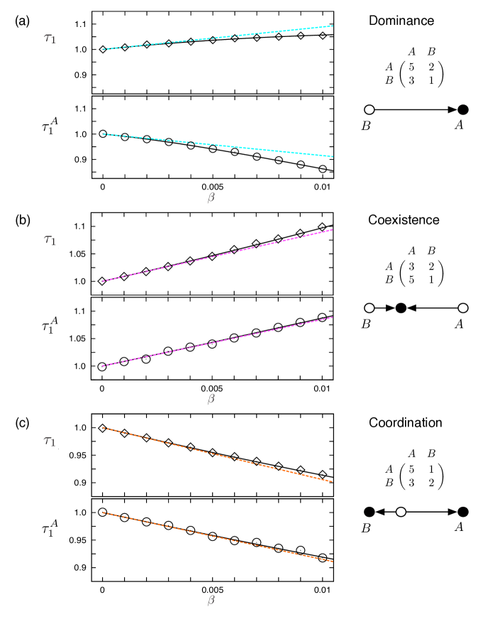
In the following, we discuss these two expressions for the three generic types of games, namely dominance of ( and ), coexistence of and ( and ) and a coordination game ( and ).
7.1 Dominance of .
Consider a game where strategy is always dominant, i. e. it obtains a larger payoff than , regardless of the fraction of in the population. This is the case for and . One special case is the Prisoner’s Dilemma with . The interesting feature of this game is that the social optimum is not the Nash equilibrium, which is . For neutral selection, a single individual goes extinct with probability . Thus, the unconditional fixation time is dominated by the extinction of . Since strategy is favored by selection, increasing the intensity of selection decreases the probability of the extinction of . Since fixation takes at least time steps, increases with increasing intensity of selection . For large , this is obvious from our equation (30), because in this case the quantity is positive. However, once extinction of becomes unlikely, increasing further will lead to a decrease of .
The discussion of the conditional fixation time is not as straightforward, because the sign of can be positive or negative. The sign of this quantity is also decisive for the evolutionary dynamics in other contexts, see e.g. [43]. When the advantage of an individual is initially large and decreases with the abundance of (), then the sign of is positive and decreases with increasing intensity of selection. But when the advantage of strategy decreases with the number of individuals (), then increases with increasing intensity of selection. However, this apparently counterintuitive phenomenon (after all, dominates ) can only be observed for weak selection. For strong selection, decreases again. These results are compatible with the observation that the conditional fixation time scales as for large [26]. In Figure -298 (a) we show a numerical example for the rescaled average times. We include averages from numerical simulations of the evolutionary process, our linear approximation as well as the exact result that can be obtained from dividing equation (14) by (18) and equation (15) by (19), respectively. The payoff matrix is chosen such that , which means that with increasing intensity of selection decreases and increases.
7.2 Coexistence of and .
As a second class, we consider games in which is the best reply to (), but is the best reply to (). Important examples for such games are the Hawk-Dove game [44] or the Snowdrift game [45]. For infinite populations, the replicator dynamics predicts a stable coexistence of and . In finite populations, the system typically fluctuates around that point until eventually, fluctuations lead to absorption in one the boundaries [46, 47]. Consequently, the conditional fixation times increase exponentially with the population size [26]. Since is negative, we also have an increase of with the selection intensity for weak selection. Further, is positive in large populations, such that also increases with the selection intensity. Figure -298 (b) shows that the divergence of the exact results is faster than the linear approximation even for weak selection.
7.3 Coordination games.
Finally, let us discuss coordination games in which and . In these games, is the best reply to and is the best reply to . The replicator equation of such systems exhibits a bistability: If the fraction of individuals is sufficiently high in the beginning, the individuals will reach fixation. Otherwise, individuals will take over the system. The stronger the intensity of selection, the less likely it is that a single individual can take over a population. Consequently, should decrease with . This also follows from our weak selection approximation: In large populations, is negative and thus decreases with the intensity of selection, see equation (30). Perhaps less intuitive, also decreases with , which results from , cf. (30). However, this is again consistent with the observation that scales as in large populations. Although the fixation probability of a single decreases with , if such an event occurs, it is faster than in the neutral case. A numerical example for this behavior is shown in Figure -298 (c).
The numerical examples indicate that the convergence radius of our weak selection expansion is of the order of , which is also known for many systems in population genetics. Although might appear small, this kind of weak selection is the most relevant limit in evolutionary biology, as evolutionary change is typically only connected with small selective differences. We stress that we have made no assumptions on the population size, such that our results are valid for arbitrary .
Our approach shows under which circumstances the general features of the game are reflected in the fixation times under weak selection. Although the weak selection expansion of the mean exit or fixation times is technically rather tedious, the resulting asymptotic behavior shows remarkable simplicity.
Acknowledgment
Financial support by the Emmy-Noether program of the DFG is gratefully acknowledged.
Appendix A Finite double sums
Here, we collect some helpful calculations for double sums as they appear in the mean exit times. An important observation is
| (32) |
for any function and . This can be seen by writing the left hand side term by term, i. e.
For the case the result is especially simple, since the first sum of the right hand side of equation (32) vanishes. This case is of special interest for the computation of under neutral selection with and for with .
Another finding for double sums with and two bounded functions and is
| (34) |
This becomes clear by resorting the terms again,
| (35) | |||||
Appendix B Fixation times under weak selection
Here, we calculate the linear corrections of the mean exit times and for the Fermi process in detail, compare equations (21) and (23). We aim at finding these times for weak selection, e.g.
| (36) |
The first term follows directly from the calculation in A, see equation (18). Our goal here is to compute the linear term .
| (37) | |||||
where we applied and . For the fixation probability under weak selection and with , we have
| (38) |
The weak selection approximation of the inverse of the transition probability , compare equation (8), yields
| (39) |
Thisleads to
| (40) | |||||
While the first two double sums can be solved with the help of A, the third term is more complicated. For this more tedious calculation, we refer to C. Eventually, the solution of the double and triple sums leads to
| (41) | |||||
where the last step is elementary. Combining this with equation (18) leads finally to the unconditional mean exit time under weak selection, equation (22).
For the conditional fixation time , the linear term reads
| (42) | |||||
The only difference compared to the unconditional fixation time, equation (37), is the fixation probability instead of . The linear term of the weak selection expansion of is given in equation (38). This yields
| (43) | |||||
Again, the first two double sums can be solved using the results from A. The third term follows from a calculation which is similar to C, but simpler. This last term reduces to
| (44) |
Finally, combining the three terms again results in
| (45) | |||||
In combination with equation (19), this results in the conditional mean exit time under weak selection, equation (24).
For completeness, we briefly repeat this calculation for the mean exit times of the frequency dependent Moran process. With the transition probabilities (25) and (26), the fixation probabilities under weak selection are identical to those of the Fermi process, see equation (20). However, the inverse transition probability is different in the weak selection regime, i. e. the linear correction is
| (46) |
Hence, for the unconditional mean exit time we have the same starting equation (37). But with equation (46) this gives
| (47) | |||||
which differs from equation (40) only in the second double sum. With the previous findings for the Fermi processes times the required calculation is straightforward and results in
| (48) |
That is, this linear correction has a different dependence on the system size .
For the conditional mean exit time the situation is similar. In difference to equation (43), the linear correction reads
| (49) | |||||
This the leads to
| (50) |
for the linear correction of the conditional mean exit times of the frequency dependent Moran process.
Appendix C Finite triple sum
Here, we calculate the triple sum from B, that require some additional steps. Our goal is to solve
| (51) |
For the sum over payoff differences, we have
| (52) |
where we introduced the function
| (53) |
which is valid for any integer . Using partial fraction expansion, , we obtain
| (54) | |||||
We solve each part separately, starting with the last one. For , we obtain with equation (32) from A
| (55) |
The second last term, , is a sum over a linear function and can be treated with any table of elementary sums, e. g. [48],
| (56) | |||||
The remaining two terms require more effort. Both terms, and have the same structure regarding functions of and . Using equation (34), we have
| (57) |
and
| (58) |
Hence, we first have to compute the sum , which reduces to the solution of elementary sums,
| (59) | |||||
Thus, solving equations (57) and (58) simplifies to solving the elementary sums with , compare [48]. With this, we have
| (60) | |||||
For , we obtain
Summing up the terms, , finally yields the result
| (61) |
Again, are the harmonic numbers. In equation (B), the reasoning is very similar, but only terms of the structure of and appear.
References
References
- [1] G. Szabó and G. Fáth. Evolutionary games on graphs. Physics Reports, 446:97–216, 2007.
- [2] J. Berg and A. Engel. Matrix games, mixed strategies, and statistical mechanics. Phys. Rev. Lett., 81:4999–5002, 1998.
- [3] G. Szabó and C. Hauert. Phase transitions and volunteering in spatial public goods games. Phys. Rev. Lett., 89:118101, 2002.
- [4] F. C. Santos and J. M. Pacheco. Scale-free networks provide a unifying framework for the emergence of cooperation. Phys. Rev. Lett., 95:098104, 2005.
- [5] C. Hauert and G. Szabó. Game theory and physics. Am. Journal of Physics, 73:405–414, 2005.
- [6] P. D. Taylor and L. Jonker. Evolutionary stable strategies and game dynamics. Math. Biosci., 40:145–156, 1978.
- [7] J. Hofbauer and K. Sigmund. Evolutionary Games and Population Dynamics. Cambridge University Press, Cambridge, 1998.
- [8] M. A. Nowak, A. Sasaki, C. Taylor, and D. Fudenberg. Emergence of cooperation and evolutionary stability in finite populations. Nature, 428:646–650, 2004.
- [9] C. Taylor, D. Fudenberg, A. Sasaki, and M. A. Nowak. Evolutionary game dynamics in finite populations. Bull. Math. Biol., 66:1621–1644, 2004.
- [10] A. Traulsen, J. C. Claussen, and C. Hauert. Coevolutionary dynamics: From finite to infinite populations. Phys. Rev. Lett., 95:238701, 2005.
- [11] G. Wild and P.D. Taylor. Fitness and evolutionary stability in game theoretic models of finite populations. Proc. Roy. Soc. Lond. B, 271:2345–2349, 2004.
- [12] L. A. Imhof, D. Fudenberg, and M. A. Nowak. Evolutionary cycles of cooperation and defection. Proc. Natl. Acad. Sci. USA, 102:10797–10800, 2005.
- [13] A. Traulsen, J. M. Pacheco, and L. A. Imhof. Stochasticity and evolutionary stability. Phys. Rev. E, 74:021905, 2006.
- [14] D. Fudenberg, M. A. Nowak, C. Taylor, and L.A. Imhof. Evolutionary game dynamics in finite populations with strong selection and weak mutation. Theor. Pop. Biol., 70:352–363, 2006.
- [15] T. Reichenbach, M. Mobilia, and E. Frey. Coexistence versus extinction in the stochastic cyclic Lotka-Volterra model. Phys. Rev. E, 74:051907, 2006.
- [16] M. Perc. Coherence resonance in a spatial prisoner’s dilemma game. New J. Physics, 8:22–33, 2006.
- [17] M. Perc and M. Marhl. Evolutionary and dynamical coherence resonances in the pair approximated prisoner’s dilemma game. New J. Physics, 8:142, 2006.
- [18] M. Perc and A. Szolnoki. Noise-guided evolution within cyclical interactions. New J. Physics, 9:267, 2007.
- [19] J. C. Claussen. Drift reversal in asymmetric coevolutionary conflicts: influence of microscopic processes and population size. European Physical Journal B, 60:391–399, 2007.
- [20] J. Cremer, T. Reichenbach, and E. Frey. Anomalous finite-size effects in the battle of the sexes. European Physical Journal B, 63(3), 2008.
- [21] A. Szolnoki and M. Perc. Coevolution of teaching activity promotes cooperation. New J. Physics, 10:043036, 2008.
- [22] J. C. Claussen and A. Traulsen. Cyclic dominance and biodiversity in well-mixed populations. Phys. Rev. Lett., 100:058104, 2008.
- [23] T. Ohta. Near-neutrality in evolution of genes and gene regulation. Proc. Natl. Acad. Sci. USA, 99:16134–16137, 2002.
- [24] H. Ohtsuki, C. Hauert, E. Lieberman, and M. A. Nowak. A simple rule for the evolution of cooperation on graphs. Nature, 441:502–505, 2006.
- [25] H. Ohtsuki, M. A. Nowak, and J. M. Pacheco. Breaking the symmetry between interaction and replacement in evolutionary dynamics on graphs. Phys. Rev. Lett., 98:108106, 2007.
- [26] T. Antal and I. Scheuring. Fixation of strategies for an evolutionary game in finite populations. Bull. Math. Biol., 36(12):1923–1944, 2006.
- [27] N. G. van Kampen. Stochastic Processes in Physics and Chemistry. Elsevier, Amsterdam, 2 edition, 1997.
- [28] S. Redner. A Guide to First-Passage Processes. Cambridge University Press, 2001.
- [29] C. W. Gardiner. Handbook of Stochastic Methods. Springer New York, third edition, 2004.
- [30] Lawrence E. Blume. The statistical mechanics of strategic interaction. Games and Economic Behavior, 4:387–424, 1993.
- [31] G. Szabó and C. Tőke. Evolutionary Prisoner’s Dilemma game on a square lattice. Phys. Rev. E, 58:69, 1998.
- [32] J. M. Pacheco, A. Traulsen, and M. A. Nowak. Co-evolution of strategy and structure in complex networks with dynamical linking. Phys. Rev. Lett., 97:258103, 2006.
- [33] A. Traulsen, J. M. Pacheco, and M. A. Nowak. Pairwise comparison and selection temperature in evolutionary game dynamics. J. Theor. Biol., 246:522–529, 2007.
- [34] S. Karlin and H. M. A. Taylor. A first course in stochastic processes. Academic, London, 2nd edition edition, 1975.
- [35] A. Traulsen and C. Hauert. Stochastic evolutionary game dynamics. In H.-G. Schuster, editor, Reviews of nonlinear dynamics and complexity. Wiley New York, 2009, arXiv:0811.3538.
- [36] M. A. Nowak. Evolutionary Dynamics. Harvard University Press, Cambridge, MA, 2006.
- [37] A. Traulsen, M. A. Nowak, and J. M. Pacheco. Stochastic dynamics of invasion and fixation. Phys. Rev. E, 74:11909, 2006.
- [38] M. E. Fisher. Diffusion from an entrance to an exit. IBM J. Res. Dev., 32:76–81, 1988.
- [39] N.S. Goel and N. Richter-Dyn. Stochastic Models in Biology. Academic Press, New York, 1974.
- [40] D. Dingli, A. Traulsen, and J. M. Pacheco. Stochastic dynamics of hematopoietic tumor stem cells. Cell Cycle, 6:e2–e6, 2007.
- [41] M. Kimura. Evolutionary rate at the molecular level. Nature, 217:624–626, 1968.
- [42] S. Lessard and V. Ladret. The probability of fixation of a single mutant in an exchangeable selection model. J. Math. Biol., 54:721–744, 2007.
- [43] C. Taylor and M. A. Nowak. Transforming the dilemma. Evolution, 61:2281–2292, 2007.
- [44] J. Maynard Smith and G. R. Price. The logic of animal conflict. Nature, 246:15–18, 1973.
- [45] M. Doebeli and C. Hauert. Models of cooperation based on the prisoner’s dilemma and the snowdrift game. Ecology Letters, 8:748–766, 2005.
- [46] J. C. Claussen and A. Traulsen. Non-Gaussian fluctuations arising from finite populations: Exact results for the evolutionary Moran process. Phys. Rev. E, 71:025101(R), 2005.
- [47] F. A. C. C. Chalub and M. O. Souza. Discrete versus continuous models in evolutionary dynamics: From simple to simpler – and even simpler – models. Math. and Comp. Modelling, 47:743–754, 2008.
- [48] R. L. Graham, D. E. Knuth, and O. Patashnik. Concrete Mathematics. Addison-Wesley, second edition, 1994.