The evolution of the Galactic metallicity gradient
from high-resolution spectroscopy of open clusters

Abstract

Context. Open clusters offer a unique possibility to study the time evolution of the radial metallicity gradients of several elements in our Galaxy, because they span large intervals in age and Galactocentric distance, and both quantities can be more accurately derived than for field stars.

Aims. We re-address the issue of the Galactic metallicity gradient and its time evolution by comparing the empirical gradients traced by a sample of 45 open clusters with a chemical evolution model of the Galaxy.

Methods. At variance with previous similar studies, we have collected from the literature only abundances derived from high–resolution spectra. The clusters have Galactocentric distances $7\lesssim R_{\rm GC}\lesssim 22$ kpc and ages from $\sim 30$ Myr to 11 Gyr. We also consider the $\alpha$-elements Si, Ca, Ti, and the iron-peak elements Cr and Ni. Cepheids trace instead the present-day Fe gradient in the inner parts of the disk.

Results. The data for iron-peak and $\alpha$-elements indicate a steep metallicity gradient for $R_{\rm GC}\lesssim 12$ kpc and a plateau at larger radii. The time evolution of the metallicity distribution is characterized by a uniform increase of the metallicity at all radii, preserving the shape of the gradient, with marginal evidence for a flattening of the gradient with time in the radial range 7-12 kpc. Our model is able to reproduce the main features of the metallicity gradient and its evolution with an infall law exponentially decreasing with radius and with a collapse time scale of the order of 8 Gyr at the solar radius. This results in a rapid collapse in the inner regions, i.e. $R_{\rm GC}\lesssim 12$ kpc (that we associate with an early phase of disk formation from the collapse of the halo) and in a slow inflow of material per unit area in the outer regions at a constant rate with time (that we associate with accretion from the intergalactic medium). An additional uniform inflow per unit disk area would help to better reproduce the metallicity plateau at large Galactocentric radii, but it is difficult to reconcile with the present-day radial behaviour of the star formation rate.

Conclusions. Our results favour a scenario where the Galactic disk is formed inside-out by the rapid collapse of the halo and by a subsequent continuous accretion of intergalactic gas

1 Introduction

The radial metallicity gradient and its time evolution provide strong constraints on our understanding of the formation and the evolution of galaxies. Detailed models of Galactic chemical evolution (GCE) have been continuously improved over the last decades (e.g., Lacey & Fall lacey (1985); Tosi tosi88 (1988); Ferrini et al. ferrini92 (1992), ferrini94 (1994); Giovagnoli & Tosi giova (1995); Chiappini, Matteucci & Gratton chiappini97 (1997); Boissier & Prantzos boissier99 (1999); Hou et al. hou00 (2000); Chiappini et al. chiappini01 (2001)). However, the issue of the time evolution of the radial abundance gradients is far from being settled unequivocally, both from a theoretical (e.g., Goetz & Koeppen goetz92 (1992); Koeppen koeppen94 (1994); Mollà et al. molla97 (1997); Henry & Worthey henry99 (1999); Chiappini et al. chiappini01 (2001)) and an observational (e.g., Friel friel95 (1995); Friel et al. friel02 (2002); Maciel maciel00 (2000); Maciel et al. maciel03 (2003); Stanghellini et al. stanghellini06 (2006)) point of view. While most GCE models are able to reproduce the present-day radial distribution of several chemical elements derived from sample objects representative of the present-day composition of the interstellar medium (ISM), such as, e.g., H ii  regions, Cepheids, super-giant stars, they generally disagree on the predicted behaviour of its time evolution.

In this respect, GCE models can be divided in two groups: models which predict a steepening of the metallicity gradient with time (e.g., Tosi tosi88 (1988); Chiappini et al. chiappini97 (1997); Chiappini et al. chiappini01 (2001)) and those which predict a flattening with time (e.g., Mollà et al. molla97 (1997); Portinari & Chiosi portinari99 (1999); Hou et al. hou00 (2000)). The main differences between the two groups of models are the efficiency of the enrichment processes in the inner andf outer regions of the Galactic disk (the star formation rate, SFR), and the nature of the material (primordial or pre-enriched) falling from the halo onto the disk (the infall).

In models of the former group the outer disk is pre-enriched by the previous evolution of the halo, and during the first Gyr its metallicity is affected very little by the relatively lower SFR in the disk. Since the infall decreases rapidly with Galactocentric radius, reflecting the strongly concentrated mass distribution in the halo, a larger amount of metal poor material falls in the central regions rather than in the outer Galactic disk. Thus, a positive metallicity gradient is initially established. When the halo collapse phase is over, the metallicity increases more rapidly in the inner disk than in the outer Galaxy, because of a combination of higher SFR at small radii and continuous dilution by infall at large radii, reversing the sign of the gradient.

In contrast, in models of the latter group, the initially vigorous star formation activity in the inner disk and the metal-poor composition of the infalling gas produce a rapid increase of the metallicity near the Galactic center. In the inner regions the metallicity increases rapidly, reaching its final value in the first 2–3 Gyr of disk evolution, whereas the enrichment of the outer disk is slower, resulting in a progressive flattening of the radial gradient. In this group of models, various infall rates have been assumed: a very rapid one simulating the formation of the disk from a monolithic collapse of the halo, or one much diluted with time, simulating a hierarchical formation of the disk by continuous infall of gas from the intergalactic medium (IGM). These rates produce different time evolution of the metallicity gradient: a rapid flattening or a uniform increase of the metallicity with essentially no change of slope, respectively (e.g., Mollà et al.molla96 (1996)).

In principle, it should be possible to discriminate between the different evolutionary scenario, by comparing the metallicity gradient of the “old” stellar population e.g., red giant branch (RGB) stars, planetary nebulae (PNe), and old open clusters (OCs), with the present-day gradient outlined, e.g., by H ii  regions, young stars (including Cepheids and giant stars) and young OCs. In external galaxies, the comparison of PN and H ii  region abundances, investigated with similar observational and analysis techniques, has given encouraging results (e.g., Magrini et al. magrini07 (2007) for the spiral galaxy M33), since PNe can be assumed at the same distance as the host galaxy.

In our Galaxy, however, the huge uncertainty on the distances to Galactic PNe restrict their use as reliable tracers of the past evolution of metallicity gradients. On the contrary, the determination of metallicities of OCs represents a reliable approach to the study of the time evolution of the metallicity gradient. OCs represent, in fact, a unique opportunity to study abundances of a large number of elements in stars of known ages and located at a wide range of well-determined Galactocentric distances. Thus, they can fully address the issue of the time evolution of the metallicity gradient, provided that a homogeneous analysis is performed.

Several spectroscopic studies of chemical abundances in OCs have been carried out during the last years, both at low- (e.g., Friel friel95 (1995); Friel et al. friel02 (2002)) and high-resolution (e.g., Carretta et al. carretta04 (2004); Carraro et al. carraro04 (2004), carraro06 (2006), carraro07 (2007); Yong, Carney & de Almeida yong05 (2005); Sestito et al sestito06 (2006), sestito08 (2008); Bragaglia et al. bragaglia07 (2008)). Different authors find different results, depending on the quality of the data, and in particular on the spectral resolution, and on the method of analysis adopted. These discrepancies especially affect metallicity gradients. Also, abundances for the farthest clusters, which are critical to determine the gradient up to very large Galactocentric distances, were not available until very recently. For example, Friel (friel95 (1995); friel06 (2006)), Carraro, Ng & Portinari (carraro98 (1998)) and Friel et al. (friel02 (2002)) suggest the presence of a negative [Fe/H] gradient, while Twarog, Ashman & Anthony-Twarog (twarog (1997)) and Corder & Twarog (corder (2001)) favor a step-like distribution of the Fe content with Galactocentric distance. Furthermore, recent results (e.g., Yong et al. yong05 (2005), Carraro et al. carraro07 (2007); Sestito et al. sestito07 (2007)) suggest that the gradient becomes flat for Galactocentric radii $R_{\rm GC}$ larger than $\sim 11-12$ kpc.

For the time evolution, evidence for variation so far has been not conclusive. The majority of studies seem to favor a slight evolution from steeper gradients in the past to shallower one at the present time. For example, Friel et al. (friel02 (2002)), based on metallicities derived from low resolution spectra, find a flattening of the overall gradient from $-0.096$ dex kpc^-1 for ages greater than 6 Gyr, to $-0.023$ dex kpc^-1 for clusters younger than 2 Gyr; similarly, Chen et al. (chen03 (2003)) derive a shallower slope for clusters younger than 0.8 Gyr than for older ones. On the contrary Salaris et al. (salaris04 (2004)) find a steeper slope for younger clusters. These discrepant results are likely due to: i) use of different and/or inhomogeneous abundance datasets; ii) the different radial regions of our Galaxy which are analyzed.

In this paper we re-address the issue of the radial metallicity gradient in our Galaxy observationally and theoretically, exploiting the availability of abundances based on high resolution spectra for several open clusters. Specifically, we collected and analyzed the most recent metallicity determinations of a large sample of OCs, considering only measurements based on high resolution spectroscopy, which by far are more reliable than those based on photometry or low resolution spectroscopy. These observations, described in Sect. 2, are compared with the results of our chemical evolution model, able to reproduce the main observational features of our Galaxy. In addition to Fe, the most recent studies (e.g., Friel et al. friel03 (2003); Carretta et al. carretta04 (2004); Friel, Jacobson, & Pilachowski friel05 (2005); Yong et al. yong05 (2005); Sestito et al. sestito06 (2006); Randich et al. randich06 (2006); Bragaglia et al. bragaglia07 (2008); Sestito et al. sestito07 (2007), sestito08 (2008)) also include the analysis of other elements. These studies allow us to investigate for the first time the radial gradient of Fe-peak and $\alpha$-elements based on the comparison of OC abundances, rather than on field stars, and model predictions. Finally, we consider the empirical gradient traced by Cepheids for the inner parts of the disk (R${}_{\rm GC}\leq 7$ kpc).

The rest of the paper is organized as follows: in Sect. 3 we describe the model; in Sect. 4 we analyze the time evolution of the radial gradient of several chemical elements, including Fe and several $\alpha$ and iron-peak elements; the abundance ratio radial behaviours are discussed in Sect. 4.2, while the results of this study are discussed in Sect. 6; in Sect. 7 we summarize our conclusions. In the Appendix we describe the details of the Galactic chemical evolution model.

2 The data sample

As discussed in Section 1, since the early study by Janes (janes79 (1979)) several works have focused on the determination of the radial metallicity gradient based on OCs. The first remarkable studies addressing the time evolution of the gradient through OC data were performed by Friel et al. (friel02 (2002)) and by Chen et al. (chen03 (2003)). The former analyzed a sample of low- and moderate-resolution data of Galactic OCs over a range in Galactocentric radius from 7 to 16 kpc. The latter was based on a collection of metallicities for a very large sample of OCs up to a distance $\leq$16 kpc from the Galactic center, whose metallicities and ages had been derived by different authors and with different methods. Therefore, whereas the catalog of Chen et al. (chen03 (2003)) represents the largest sample of OCs so far collected to study the gradient, it is greatly inhomogeneous.

In the last few years, and after the two studies mentioned above, thanks to state-of-the-art multiplex facilities on 8m class, the number of OC with secure metallicity determinations from high-resolution spectroscopy has greatly increased. Also, and most important, it has been possible to extend metallicity determinations to OCs in the outer disk, beyond 15-16 kpc from the Galactic center. Finally, abundances of other elements besides iron have been determined.

In this context, the strength of our data sample is that it combines the largest available sample of high-resolution observations of OCs, including OCs with Galactocentric distances between $\sim 7$ and 22 kpc, together with a homogeneous treatment of their age derivation, attaining larger Galactocentric distances than in previous samples.

Our dataset of OCs (see Table 1) is a collection of samples analyzed by different authors in the literature. Table 1 lists in Cols. 1 and 2 the sample clusters and their Galactocentric distances $R_{\rm GC}$, taken from Friel et al. (friel02 (2002)), when available, otherwise from Friel (friel95 (1995), friel06 (2006)); in the few cases when R_GC from Friel was not available, we calculated this quantity using the cluster distance given in the papers quoted in the table and assuming a solar Galactocentric distance of 8.5 kpc, consistent with Friel et al.

In Col. 3 we list the ages of the sample clusters. Since they are retrieved from different sources, a unique and/or consistent age determination for them is not available. As is well known, age is very sensitive to the method employed, to the adopted stellar models in the case of isochrone fitting, and it can vary significantly from one study to another of the same cluster. In order to obtain a homogeneous set of ages for the oldest clusters (ages $\geq 0.5$ Gyr), we decided to use the morphological age indicator $\delta$V (Phelps et al. phelps94 (1994)) and the metallicity-dependent calibration of Salaris et al. (salaris04 (2004)). For most of the sample clusters $\delta$V is available from the literature; when not available, we obtained this quantity from available color-magnitude diagrams. Alternatively, we determined $\delta$(B-V) and derived $\delta$V from it (see again Phelps et al.). Note that for the calibrating clusters of Salaris et al. (salaris04 (2004)) we directly used their age determination. For the younger clusters (the first seven lines of Table 1), we used the most recent age determinations available in the literature, such as those obtained with the lithium depletion boundary method. Use of non-homogeneous age determinations for young clusters will not affect our results and discussion, given our classification of the OCs in three major age bins (see below).

Information on the observations and the analysis techniques is listed in Cols. 5, 6, 7, 8: specifically, we give the signal to noise ratio (S/N), the resolving power (R), the number and type of stars analyzed (giant or dwarf stars), and the method of analysis. The values of [Fe/H] and their errors, references to the observations and abundance analysis are listed in Cols. 9 and 10. As the table shows, the values of R and S/N cover a rather wide interval, although for most samples the resolution is R$\sim$30,000–40,000. The metallicities are more often derived through equivalent width measurements, although in a few cases spectral synthesis was employed. The analysis is based on giant stars for most of the intermediate age and old clusters, while for the young, more close-by cluster main sequence stars have been used. As discussed by Randich et al. (randich06 (2006)) for M67 and Pasquini et al. (pasquini (2004)) for IC4651, this should not introduce any major bias for the elements considered here. The numbers of stars used in each analysis range from 1 to 15, with the exception of the very rich set by Paulson et al. (paulson03 (2003)) for the Hyades (55 dwarf stars).

In order to check whether (and to what extent) use of different abundance scales might introduce spurious trends or increase the dispersion, we compared different abundance measurements for the same cluster. Considering only the most recent studies based on high resolution, we found 11 cases with more than one [Fe/H] determination available. The difference between the [Fe/H] values does not depend on [Fe/H] itself and the average is rather small; namely, $\Delta$[Fe/H]=0.12 dex with a standard deviation of 0.08 dex. This value is somewhat larger (a factor of $\sim 2$) than the typical error in [Fe/H] of most clusters; however, we believe that it is small enough not to affect our results in a significant way. For other element abundances, very few clusters have more than one determination; these studies indicate that the differences in [X/H] are likely larger and can be as large as 0.2 dex and might introduce a certain amount of scatter in the observed distributions.

3 The chemical evolution model

The model adopted in this work is a generalization of the multi-phase model by Ferrini et al. (ferrini92 (1992)), originally built for the solar neighborhood, and subsequently extended to the entire Galaxy (Ferrini et al. ferrini94 (1994)), and to other disk galaxies (e.g., Mollà et al. molla96 (1996), molla97 (1997); Mollà & Diaz molla05 (2005); Magrini et al. magrini07 (2007)). We refer to Ferrini et al. (ferrini92 (1992),ferrini94 (1994)), Mollá et al. (molla96 (1996)), and to Magrini et al. (magrini07 (2007)) for a detailed description of the general model. The main assumptions of our model are that the Galaxy disk is formed by infall of gas from the halo and from the interstellar medium. The adopted infall has an exponentially decreasing law. This produces an inside-out formation scenario where the inner parts of the disk evolve more rapidly than the outer ones. We consider also an alternative parametrization of the infall including a constant amount of gas per unit area in addition to the exponentially decreasing law. This latter parametrization is useful in reproducing the metallicity gradient, but resulted in an enhanced star formation rate in the outer regions.

In the Appendix the overall content of our model and in particular the specific assumptions and parameterizations we used to reproduce the Galactic disk properties are described in detail.

4 Radial gradients: comparison between models and observations

In Figs. 1, 3, 4, and 5, we compare abundances in OCs with the predictions of the model described in the Appendix for the $\alpha$-elements Si, Ca, Ti, and the iron-peak elements, Fe, Ni, and Cr. In general, the observed abundance distributions show a two-slope feature with a change from a steep gradient for $R_{\rm GC}\lesssim 11-12$ kpc and a flat plateau at greater distances, at least in the two older age bins. For simplicity, we will assume 12 kpc as the threshold Galactocentric distance to distinguish the inner regions from the outer plateau. We caution that this value is rather arbitrary since the samples in each age bin are limited and there is a lack of OC data in the radial range 12–15 kpc which would allow us to better constrain this value. We note however that our conclusions would not change by assuming a smaller (e.g., 11 kpc) or larger (e.g., 13 kpc) radius. For the Cepheids a change of slope also is seen at 7 kpc, with a steepening of the slope for $R_{\rm GC}<7$ kpc.

In the following we will discuss separately the iron and other element gradients. For a better comparison with the chemical model, we have divided the cluster ages in three bins, namely (i) age less than or equal to 0.8 Gyr, (ii) 0.8 Gyr$<$age$\leq 4$ Gyr, and (iii) 4 Gyr$<$age$\leq$ 11 Gyr.

4.1 Iron

In Fig. 1 and 2 we show the distribution of [Fe/H] of OCs and Cepheids as a function of the Galactocentric distance $R_{\rm GC}$, and compare it with the [Fe/H] behaviour predicted by our model. For the Fe abundances of the Cepheids we have used the gradient derived by Andrievsky et al. (andri04 (2004)) and Lemasle et al. (lemasle07 (2007)). We recall that the Cepheids represent a young population; thus their data can be compared only with the current model gradient, while OC data allow a comparison with the model predictions at different epochs.

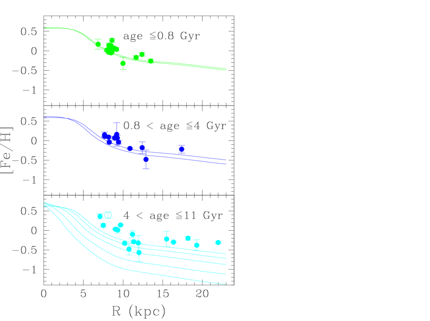
Figure 1: Gradient of [Fe/H]: comparison between high-resolution data of OCs with the model decribed in the Appendix. Different panels show abundances for different age bins: top (panel 1), ages $\leq$0.8 Gyr; middle (panel 2), ages $0.8\leavevmode\nobreak\ \mbox{Gyr}<\mbox{age}\leq 4\leavevmode\nobreak\ \mbox{Gyr}$; bottom (panel 3), ages $4\leavevmode\nobreak\ \mbox{Gyr}<\mbox{age}\leq 11\leavevmode\nobreak\ \mbox{Gyr}$. The models adopted to compare with observations are for 0 and 1 Gyr ago (panel 1), 1 and 4 Gyr ago (panel 2), and 4, 6, 8, 10, 11 Gyr ago (panel 3).

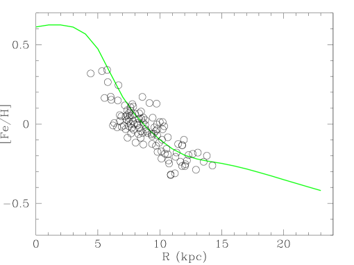
Figure 2: Gradient of [Fe/H]: comparison between Cepheid data (Andrievsky et al. andri04 (2004)) and our current model.

The shape of the Fe gradient of OCs, at least in the most populated age bin (age between 4 and 11 Gyr) is characterized by a negative slope at short radii and a change of slope at around $\sim$11-12 kpc, resulting in a plateau at larger distances. This behaviour is qualitatively similar to that of Cepheid data, although the latter cover an inner part of the disk and show a change of slope around 7 kpc, but do not extend beyond 15 kpc.

More specifically, it is useful to analyze in detail the gradient in the three radial zones selected, namely $4\leavevmode\nobreak\ \mbox{kpc}\lesssim R_{\rm{GC}}\lesssim 7\leavevmode\nobreak\ \mbox{kpc}$ (region I), $7\leavevmode\nobreak\ \mbox{kpc}\lesssim R_{\rm{GC}}\lesssim 12\leavevmode\nobreak\ \mbox{kpc}$ (region II), $12\leavevmode\nobreak\ \mbox{Kpc}\lesssim R_{\rm{GC}}\lesssim 22\leavevmode\nobreak\ \mbox{kpc}$ (region III). From Table 3 and Fig. 2 it is evident that the current gradient outlined by the metallicity of Cepheids is very steep in region I, where, unfortunately, no high-resolution OC data are available. In region II, the gradient traced by Cepheids ($-0.051$ and $-0.044$ dex kpc^-1 according to Lemasle et al. lemasle07 (2007) and Andrievsky et al. andri04 (2004), respectively) is consistent with that outlined by the youngest OCs ($-0.053$ dex kpc^-1 –see Sect. 6). Finally, as already suggested by the most recent papers (e.g. Yong et al. yong05 (2005); Carraro et al. carraro04 (2004), carraro07 (2007); Sestito et al. sestito08 (2008)), data from of OCs in region III indicate a very flat outer gradient, with a slope consistent with zero at all epochs (see also Sect. 6).

As noted by Andrievsky et al. (andri04 (2004)), the existence of a discontinuity in the metallicity gradient at $\sim$11–12 kpc, observed for both Cepheid and OCs data, is predicted and explained by two chemical evolution models. One of them is the model proposed by Andrievsky et al. (andri04 (2004)) themselves, and the other is the model C presented by Chiappini et al. (chiappini01 (2001)). In particular, Andrievsky et al. (andri04 (2004)) assume that the SFR is a combination of two components: one proportional to the gas surface density, and the other depending upon the relative velocity of the interstellar gas and spiral arms. However, their model predicts a strong decrease in metallicity beyond $\sim 14$ kpc, whereas the observed gradient from OCs is flat up to $\sim 22$ kpc. On the other hand, Chiappini et al. (2001) assume two main accretion episodes in the lifetime of the Galaxy, the first one forming the halo and bulge and the second one forming the thin disk. Both episodes are described by exponential laws. Their model C does not assume any threshold in the gas density during the halo/thick-disk phase, and thus allows the formation of the outer plateau from infalling gas enriched in the halo.

Figs. 1 and 2 show that our model is also able to reproduce the flat gradient at large Galactocentric distances. This is explained in the framework of our chemical evolution model by the radial dependence of the infall rate (exponentially decreasing with radius) which, combined with the gas distribution in the halo, results in a gas falling into the disk rapidly in the regions with R$\lesssim$12 kpc and at a almost constant rate in the outer regions (see Fig. 12). In addition, the radial dependence of the star and cloud formation processes, that are more efficient in the inner regions, produces a higher SFR in the inner regions, resulting in a higher metal production. In contrast, in the outer disk, the low metallicity of the infalling gas and the low SFR contribute to maintain a flat and slowly evolving metallicity gradient.

To reproduce a completely flat gradient in the external regions, as indicated by the older OCs, our model would need an additional accretion of material uniformly falling onto the disk. This however would result in an inconsistent behaviour of the current SFR, predicting higher SFR in the external regions. We then considered several possible events that could explain the trend of the metallicity gradient traced by older OCs. The plateau is most evident only in the older group of OCs, and thus it could be related to peculiar episodes in the past history of the Galaxy. The outer plateau could be a signature of a past merger at high radii with pre-enriched material, or similarly to what is suggested by the model of Chiappini et al. (chiappini01 (2001)), of a gas halo already enriched. In this case it would not be necessary to modify the radial profile of the SFR to have higher element abundance at high radii, since the inflow of material would bring a higher content in metals. Alternatively, it could be caused by a strong episodic merger in the past with clouds/galaxies at high Galactocentric radii. Sporadic episodes of mergers with galaxies at large Galactocentric radii, more frequent in the past history of our Galaxy, would not strongly affect the current SFR and would explain the outer plateau in metallicity. However, fine tuning of the composition of the merger would be needed to reproduce the exact plateau value in iron and the distribution of other elements (see next section).

4.2 Iron-peak- and $\alpha$-elements

Two iron-peak elements, Ni and Cr, and three $\alpha$-elements (Si, Ca, and Ti) have been measured in a large number of OCs belonging to the selected sample. Their gradients are plotted in Figs. 3, 4 and 5. The radial gradients are in most cases very similar and also very close to the iron gradient, with a negative slope at low radii and a slightly decreasing distribution at larger distances (see Table 3). Note that in a few cases we were not able to derive a quantitative value for the slope, due to low statistics and/or to the small range of R_GC covered by the clusters with available abundances. Also, in two of cases (Ca and Cr) the slope in the 7–12 kpc range in the intermediate-age bin is consistent with 0, at variance with that of Fe. For all elements, however, the slope in the oldest age bin in the 7–12 kpc interval is very similar to the slope of [Fe/H]. This similarity is expected in our model because the metallicity gradient is determined for all elements by the radial dependence of the SFR and the infall.

In order to reproduce the absolute mean values of $12+\log({\rm Cr/H})$, we have assumed a production of Cr from SN Ia lower by a factor of $\sim 2$ than that by Iwamoto et al. (iwamoto99 (1999)), while [Ni/H], [Ca/H], [Si/H], and [Ti/H] values are all well reproduced using the original yields by Iwamoto et al. (iwamoto99 (1999)). The best agreement of the model prediction with the observed time and radial behaviours of the Ti abundance is obtained adopting stellar yields from massive stars higher by a factor of $\sim 2$ than those computed by Chieffi & Limongi (chieffi04 (2004)). This correction is in agreement with the empirical stellar yields adopted by François et al. (francois04 (2004)).

In summary, all elements under consideration, in particular in the most represented age range, $4\leavevmode\nobreak\ \mbox{Gyr}\lesssim\mbox{age}\lesssim 10$ Gyr, confirm the existence of a steep gradient in the inner regions and a change of slope at around $\sim$12 kpc with a flattening of the gradient towards the outer regions.

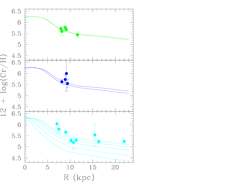
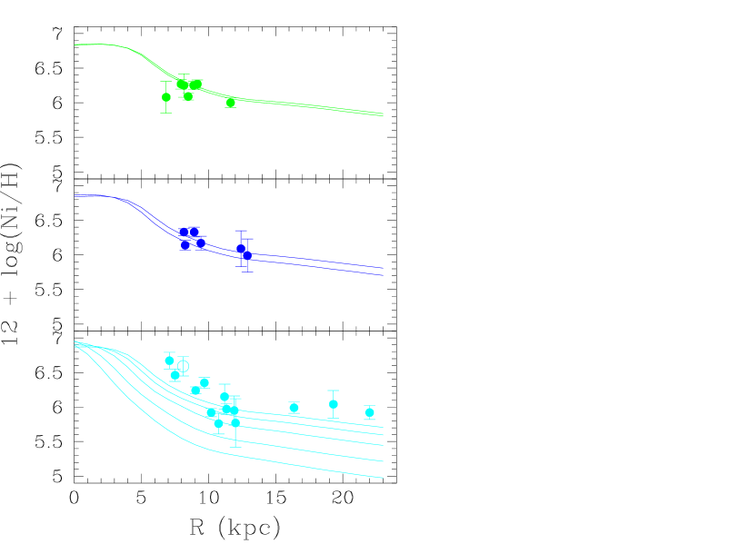
Figure 3: Radial gradients of $12+\log({\rm Cr/H})$ and $12+\log({\rm Ni/Fe})$: comparison between high-resolution data of OCs with our model. Symbols and line-types are as in Fig. 1. These figures are available in electronic form only.

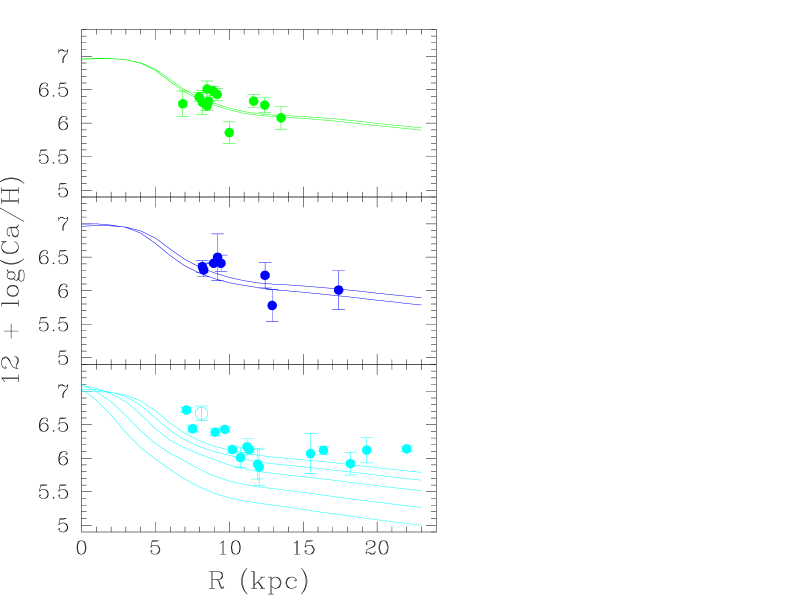
Figure 4: Radial gradients of $12+\log({\rm Si/H})$ and $12+\log({\rm Ca/H})$: comparison between high-resolution data of OCs with our model. Symbols and line-types are as in Fig. 1. These figures are available in electronic form only.

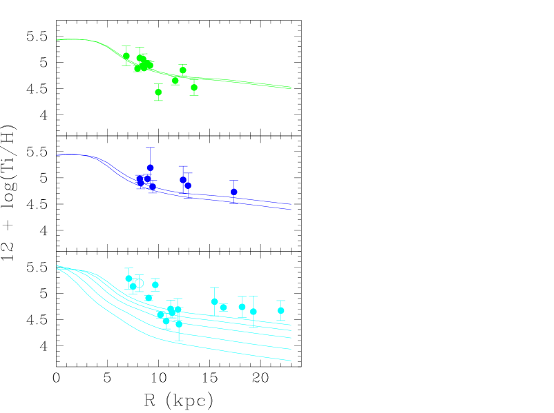
Figure 5: Radial gradient of $12+\log({\rm Ti/H})$: comparison between high-resolution data of OCs with our model decribed. Symbols and line-types are as in Fig. 1. These figures are available in electronic form only.

5 [X/Fe] radial gradients

Although abundance ratios are less model-dependent than absolute abundances (see e.g. Matteucci & Chiappini matteucci04 (2005)), nevertheless they are affected by assumptions on stellar nucleosynthesis processes, the IMF, and stellar lifetimes. In particular, abundance ratios involving elements produced on short timescales by massive stars dying as SN II, like $\alpha$-elements, and elements produced on longer timescales by e.g. SN I, like iron-peak elements, allow us to study the role of different types of supernovae in the chemical history of the Galaxy.

In Fig. 6, 7, and 8, we compare the values [X/Fe] from high-resolution data with the predictions of the model. The production of iron-peak elements is dominated by SN Ia. Since iron has the same SN Ia origin, the ratios [X/Fe] of these elements are not expected to show any evident temporal evolution.

Two iron-peak elements, Ni and Cr, have been measured in a large number of clusters belonging to our sample. Both elements show an almost constant average value, close to the solar one at all ages. The absolute mean values of [Cr/Fe] are reproduced assuming a production of Cr from SN Ia lower by a factor of $\sim 2$ than that by Iwamoto et al. (iwamoto99 (1999)), while [Ni/Fe] values are well reproduced using the original yields by Iwamoto et al. (iwamoto99 (1999)).

Models and observations of both elements, in particular in the most represented age range, $4\leavevmode\nobreak\ \mbox{Gyr}\lesssim\mbox{age}\lesssim 11$ Gyr, confirm a constant behaviour of [X/Fe] with Galactocentric radius. We recall that typical formal uncertainties in [X/Fe] vary from 0.01 to 0.15 dex. In the case of Ni lower values of [Ni/Fe] are observed in the few young clusters analyzed than in the older cluster sample. Also the [Cr/Fe] of some clusters in the old-age bin have lower values than expected from the model. Both these behaviours are not reproduced by the model, and they could be statistical variations, not significant, due to the small sample of clusters with these measurements.

Data for the three $\alpha$-elements observed in the high-resolution sample of OCs (Si, Ca, and Ti) indicate a rather flat distributions with Galactocentric distance, and nearly solar [$\alpha$/Fe] values, slightly higher for older clusters. The largest contribution to the production of Si, Ca, and Ti comes from massive stars with $M>8M_{\odot}$ (e.g., Chieffi & Limongi chieffi04 (2004)) while small amounts of these elements are also produced by SN Ia (e.g., Iwamoto et al. iwamoto99 (1999)). This is especially true for Ca: for example, SN Ia models by Iwamoto et al. (iwamoto99 (1999)) predict a typical synthesized mass of Ca of about 0.02–0.03 $M_{\odot}$ per SN Ia, to be compared with the $0.016\leavevmode\nobreak\ M_{\odot}$ of Ca produced by a star of 25 M_⊙ of solar metallicity (cf. Chieffi & Limongi chieffi04 (2004)). Thus the production of Ca and Fe, integrated over the IMF, occur on comparable time scales, and the [Ca/Fe] gradient does not show any evident temporal evolution. Silicon, on the other hand, being mostly produced by rapidly evolving massive stars, shows high values compared to Fe in the past, and a more rapidly increasing [Si/Fe] radial gradient than e.g., the [Ca/Fe] gradient, as suggested by e.g., Cescutti et al. (cescutti06 (2006)). These temporal and spatial behaviours are well reproduced by the model, that also predicts a slight enhancement of [$\alpha$/Fe] in the outer regions, due to the different spatial location of SN II and SN Ia. This is partially confirmed by the limited number of high-resolution observations of OCs.

Titanium shows a large dispersion with cluster age, similarly to the one observed for [Si/Fe]. The best agreement of the model prediction with the observed temporal and radial behaviours of the Ti abundance is obtained adopting stellar yields from massive stars higher by a factor of $\sim 2$ than those computed by Chieffi & Limongi (chieffi04 (2004)). This correction is in agreement with the empirical stellar yields adopted by François et al. (francois04 (2004)).

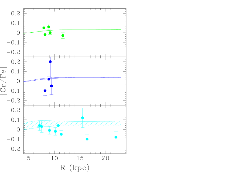
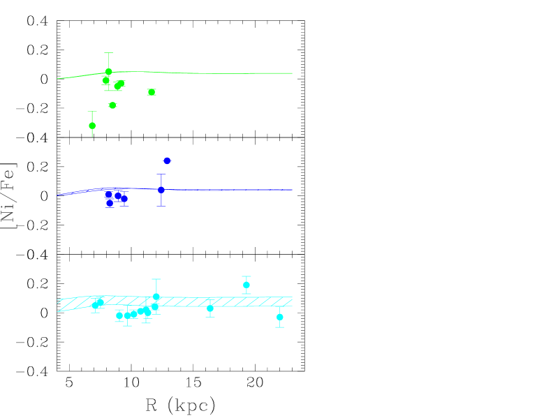
Figure 6: Radial gradients of [Ni/Fe] and [Cr/Fe]: comparison between high-resolution data of OCs with our model. Different panels show abundances for different age bins: top (panel 1), ages $\leq$0.8 Gyr; middle (panel 2), ages $0.8\leavevmode\nobreak\ \mbox{Gyr}<\mbox{age}\leq 4\leavevmode\nobreak\ \mbox{Gyr}$; bottom (panel 3), ages $4\leavevmode\nobreak\ \mbox{Gyr}<\mbox{age}\leq 11\leavevmode\nobreak\ \mbox{Gyr}$. The models adopted to compare with observations are for 0 and 1 Gyr ago (panel 1), 1 and 4 Gyr ago (panel 2), and 4, 11 Gyr ago (panel 3). The shaded regions indicate the area between the two models shown in each panel. These figures are available in electronic form only.

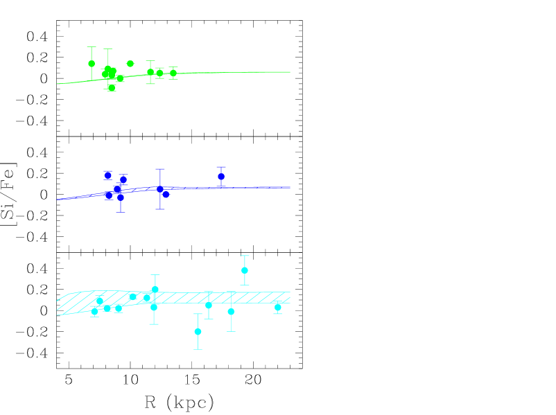
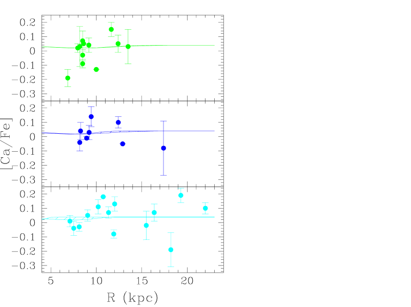
Figure 7: Radial gradients of [Si/Fe] and [Ca/Fe]: comparison between high-resolution data of OCs with our model. Symbols and line-types are as in Fig. 6. These figures will be published in the electronic form only.

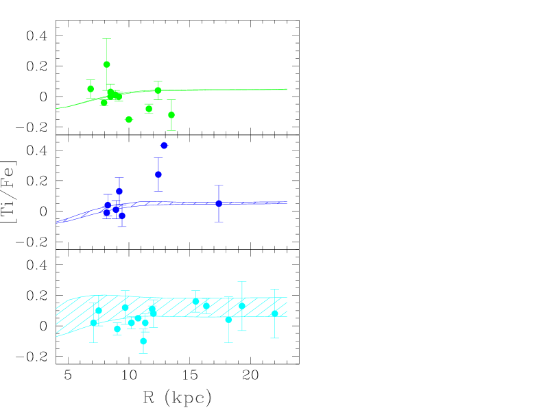
Figure 8: Radial gradient of [Ti/Fe]: comparison between high-resolution data of OCs with our model. Symbols and line-types are as in Fig. 6. These figures are available in electronic form only.

As described in the Appendix, with our adopted model parameters (infall, star and cloud formation efficiencies, chemical yields, etc.) the best agreement of the theoretical gradients with the observations is obtained using the IMF by Kroupa et al. (kroupa93 (1993)). We also checked several other parameterizations of the IMF: assuming the “best” values (i.e. measured independently) for the various efficiencies of star and cloud formation at solar radii, we have varied the adopted parametrization of the IMF. A good agreement was also obtained with the IMFs by Ferrini et al. (ferrini90 (1990)) and Scalo (scalo86 (1986)). These parameterizations are characterized by a lower number of massive stars when compared e.g., with the Salpeter (salpeter55 (1955)), Scalo (scalo98 (1998)), and Chabrier et al. (chabrier03 (2003)) IMFs. The high-resolution OC abundances of $\alpha$-elements seem to weaken the use of these other parameterizations that in fact result in an overproduction of massive stars, and, consequently, a production of $\alpha$-elements greater than observed. For example, a Salpeter IMF would result in an overproduction of Ti in the model of $\sim 0.3$ dex with respect to the observations.

6 The time evolution of the metallicity gradient

Table 2: Average [Fe/H] from OC data of different epochs and radial regions (see the text for the definition of radial regions).

age (Gyr)	Region II	Region III
$<0.8$	$0.016\pm 0.14$	$-0.17\pm 0.12$
0.8–4	$0.05\pm 0.11$	$-0.29\pm 0.16$
4–10	$-0.04\pm 0.29$	$-0.33\pm 0.13$

In their paper, Maciel et al. (2006) showed the results on the time evolution of the [Fe/H] gradient obtained by several authors, both from models (Hou et al. hou00 (2000), Chiappini et al. chiappini01 (2001)) and from observations (PNe by Maciel et al. 2006, OCs by Friel et al. 2002, Chen et al. 2003, and H ii regions, Cepheids, OB stars from several authors, see references therein). The metallicity gradient was computed over the whole disk. However, as already remarked, the gradient does not have a constant slope over the whole disk, and, thus, a direct comparison with our data is difficult to obtain.

Therefore we compared our results with the samples of OCs by Friel et al. (2002) and Chen et al. (2003) in the same radial regions. Their samples were discussed in the previous sections. In summary, they differ from our sample in data quality (high-resolution spectroscopy vs. low-resolution spectroscopy and/or photometry) and radial range (they extend up to $\sim$16 kpc, while our sample extends up to 22 kpc). The OCs located at high Galactocentric radius are fundamental in determining the slope in the older and intermediate age bin. In order to compare with the results of Friel et al. (2002) and Chen et al. (2003) we have re-computed the slope of the older and intermediate age bins for $R_{GC}\leq 16$, obtaining a slope for the cumulative sample of -0.067 dex kpc^-1, and for only the old bin of -0.079 dex kpc^-1, in closer agreement with their results: -0.075 dex kpc^-1 for the sample of Chen et al. (2003) with ages $>$0.8 Gyr and -0.075 dex kpc^-1 for the sample of Friel et al. (2002) with ages $>$4 Gyr. This points out the importance of OCs at larger Galactocentric distances for a correct determination of the outer gradient.

The comparison with PNe is more tricky. The accuracy of the Galactic metallicity gradient derived for PNe has been debated for a long time because of the large uncertainties on PN distances. Recent results (Stanghellini et al. stanghellini06 (2006), Perinotto & Morbidelli perinotto06 (2006)) have shown very different gradients for the Galactic PN population than previous results. At variance with Maciel et al.’s results, Stanghellini et al. (stanghellini06 (2006)) and Perinotto & Morbidelli (perinotto06 (2006)) found an almost flat gradient at all epochs. On the other hand, some other recent works find steeper gradients (e.g., Pottasch & Bernard-Salas pottasch06 (2006); Maciel & Costa maciel08 (2008)) pointing to the need for an accurate determination of the age in order to measure gradients. The main differences among these works are the adopted distance scales, demonstrating how this choice can affect the estimate of the metallicity gradient, in conjunction with different age estimates for the PN progenitors. Thus a faithful determination of the Galactic metallicity gradient from PNe is far from being obtained.

A more appropriate way to compare the chemical evolution model with observations is to divide the Galaxy in several radial regions. In Tables 2 and 3 we list the the average abundances of iron in each age bin and radial region, and the best-fit slopes in the three radial regions. The latter were computed through a weighted fit procedure for the OCs and taken from Andrievsky et al. (andri04 (2004)) and Lemasle et al. (lemasle07 (2007)) for the Cepheids. The slopes of the models are also shown. As anticipated above, three age bins were considered: age less than or equal to 0.8 Gyr, in the first panel; $0.8<\mbox{age}\leq 4$ Gyr, in the second panel; and $4<\mbox{age}\leq 11$ Gyr in the third panel. For OCs with ages between 4 Gyr and 11 Gyr, we excluded from the calculation of gradient the metal-rich cluster NGC 6791 (marked with an empty circle in Figs. 1, 3, 4,5), because it was probably born in a different place in the disk or could even have been captured by our Galaxy during a merger event (Carraro et al. carraro06 (2006), but see also Bedin et al. bedin06 (2006) for a contrasting view). Thus the age range for our further analysis is between 4 Gyr and 10 Gyr.

First, we note that, although it is well known that a strict age-metallicity relationship does not hold in the Galactic disk, a tendency is present for older OC to have on average lower metallicities. Second, each radial region shows a different behaviour due to the distinct ratios of SFR and infall. To better analyze the time evolution of the metallicity gradients, we plot in Fig. 9 the slopes of the gradient for the specific case of iron, the best studied element, in the three radial regions defined above. Similar behaviours are observed also for the other elements analyzed in this study.

As there are no observations of OCs in region I, it is not possible to obtain the time evolution of the gradient in this region. In region II, our sample of OCs does not show any conclusive evidence for flattening with time of the slope of the gradient, although the present time gradient seems slightly flatter then the gradient in the two older age bins. Finally, in region III, the OC metallicities produce a gradient consistent with a zero slope at all epochs.

Our data have allowed us to consider the time evolution in different regions of the disk, showing that in the $\sim 7$–22 kpc interval no marked evolution is present.

The observations of Cepheids by Andrievsky et al. (andri04 (2004)) (see Table 3 and filled squares in Fig. 9) show a good agreement with the absolute [Fe/H] predicted by the model in regions I, II, and III at the present time (see Table 3). In region I, the model predicts a flattening of the metallicity gradient from the past epochs to the present time that cannot be tested because only Cepheid data are available in this region; in regions II and III it predicts an overall increase of metallicity at all radii but no significant change in the slope of the gradient (see Fig. 9).

This can be understood as follows. In our model, the inner part of the disk is built by the rapid collapse of the halo, whereas the outer parts by the continuous slow accretion of intergalactic gas. In the inner disk, a steep chemical gradient is initially established by the strong concentration of infalling gas (see eq. 7), on a timescale probably of the order of a few Gyr or less (OCs are not able to constrain the chemical evolution of the gradient for the first $\sim 5$ Gyr of evolution of the Galaxy). The model predictions indicate that this initial gradient is preserved in the subsequent evolution of the disk.

Turbulent mixing of the interstellar gas seems to be inefficient in smoothing the initial metallicity gradient over the lifetime of the Galaxy, in agreement with theoretical estimates; for example, according to Talbot & Arnett (talbot73 (1973)), the timescale for mixing a region of a radial extent of 5 kpc like Region II is about $75$ Gyr. Also the role of large-scale radial flows, often invoked in the chemical evolution of disk galaxies, seems quite marginal, since their effect is to steepen the metallicity gradient (Lacey & Fall lacey (1985); Tosi tosi88 (1988); Portinari & Chiosi portinari00 (2000)), contrary to observational evidence. However Friedli (friedli98 (1998)) found that flows induced by bars can flatten the gradient. In the outer disk, on the other hand, accretion of intergalactic gas and disk evolution occur almost independently of radius, and the metallicity gradient remains flat.

We note that the slope of older OCs is significantly affected by the presence of a number of old clusters located at low Galactocentric distances with solar or super-solar metallicities. Old clusters have had enough time to move along their orbits, and the possibility exists that they were actually born in inner regions far from their present location. Although it seems unlikely that all old clusters with (over)-solar metallicities have different birthplaces, we stress that knowledge of the orbits of these older OCs, and thus their previous location, would help in definitively settling the issue. Also, a few clusters located at distances of 11-12 kpc are present with [Fe/H] somewhat below the plateau value observed at larger Galactocentric distances and characterized by large error bars. New observations for these clusters should be obtained in order to better constrain the slope of the gradient. Finally, metallicity determinations should be performed for both young and old clusters located at Galactocentric distances lower than $\sim 7$ kpc.

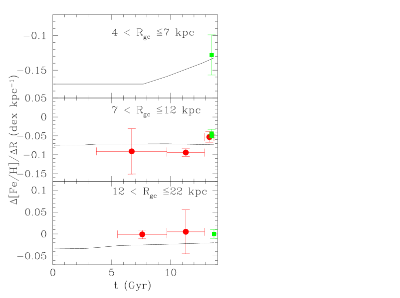
Figure 9: Time evolution of the slope of the iron gradient in the three radial region analyzed: $4$ kpc $\lesssim R_{\rm{GC}}\lesssim 7$ kpc (region I), $7$ kpc $\lesssim R_{\rm{GC}}\lesssim 12$ kpc (region II), $12$ kpc $\lesssim R_{\rm{GC}}\lesssim 22$ kpc (region III). Continuous lines are the slopes of the model gradients approximated with a linear fit. Filled squares are the slopes of the gradients of Cepheids. Filled circles represent the slopes of OC gradients with their uncertainties in the three age bins, as in Table 3.

7 Summary

s We have assembled a homogeneous sample of abundances in OCs from high-resolution spectroscopic data and compared it to the results of a GCE model. We examined in particular the radial gradients of Fe/H, Si/H, Ca/H, Ti/H, Ni/H, and Cr/H, and also their [X/Fe] gradients at different epochs during the lifetime of the Galaxy. We have divided our data into three age bins and three radial regions. Our main results are the following:

• From the observations of OCs and Cepheids (see Table 3), we find that the metallicity gradients of all the elements analyzed are very steep at low Galactocentric radii, in particular for $R_{\rm GC}\lesssim 7$ kpc. The gradients show a change of slope around 7 kpc, and further flattening at about 11–12 kpc, resulting in a metallicity plateau in the outer regions.

• The combination of the observations of Cepheids and OCs allow us to follow the time evolution of the metallicity gradient and to compare it with the results of a GCE model. The time evolution of the gradient can be followed where observations of OCs with different ages are available for $R_{\rm GC}>7$ kpc. At Galactocentric radii $7$ kpc $\lesssim R_{\rm GC}\lesssim 12$ kpc the combined observations of Cepheids and OCs suggest that the slope of the metallicity gradient has not changed significantly over the past $\sim 10$ Gyr; if anything, the gradient has flattened with time, as also suggested by the model for $R_{\rm GC}<7$ kpc. For $12\leavevmode\nobreak\ \mbox{kpc}\lesssim R_{\rm GC}\lesssim 22$ kpc, OCs belonging to different epochs and Cepheids all suggest a flat metallicity distribution.

• The GCE model that better reproduces the data is characterized by an inside-out formation of the disk. The infall of gas is represented by an exponential law which, combined with the distribution of gas in the halo, produces a rapid collapse in the regions with R$\lesssim$12 kpc and a uniform accretion in the outer regions. The inner regions are rapidly evolving due to the higher infall and SFR, while the outer parts evolve more slowly. The metallicity in the outer disk increases uniformly at all radii without a marked change of slope of the gradient. Peculiar episodes of mergers in the past history of the Galaxy would explain the outer metallicity plateau indicated by the older clusters.

Table 1: Open clusters included in our sample. We list in Col. 1 the cluster name, in Col. 2 the cluster age, in Cols. 3 and 4 the Galactocentric radius and its reference (an asterisk indicate that we computed R_GC assuming the cluster distance given in the quoted reference). In Cols. 5, 6, 7, 8, 9, and 10 we list the main properties of the observations and of the analysis: the signal to noise ratio, the resolving power, the number and type of stars analyzed, the adopted method (Equivalent widths, EW, or spectral synthesis), the iron abundance with its error, and the reference.

Cluster	Age	$R_{\rm{GC}}$	Ref.	S/N	R	N.Stars	Method	[Fe/H]	Ref.
	(Gyr)	(kpc)	($R_{\rm{GC}}$)						([Fe/H])
IC4665	0.025	8.18	Manzi et al. (manzi08 (2008))∗	30-150	60,000	18,dwa	Synt	$-0.03\pm 0.04$	Shen et al.. (shen (2005))
IC2602	0.035	8.49	WEBDA∗	30-100	18,000-44,000	9,dwa	EW	$-0.05\pm 0.05$	Randich et al. (2001)
IC2391	0.053	8.50	WEBDA∗	30-100	18,000-44,000	4,dwarfs	EW	$-0.03\pm 0.07$	Randich et al. (2001)
Blanco 1	0.1-0.15	8.50	Friel (friel06 (2006))	70-100	50,000	8,dwa	EW	$+0.04\pm 0.04$	Ford et al. (ford05 (2005))
Pleiades	0.125	8.60	Friel (friel06 (2006))	70	45,000	15,dwa	EW	$-0.03\pm 0.02$	Boesgaard & Friel (boesgaard90 (1990))
NGC6475	0.220	8.22	Robichon et al. (robichon99 (1999))∗	50-150	29,000	13,dwa	EW	$+0.14\pm 0.06$	Sestito et al. (sestito03 (2003))
M11	0.250	6.86	Gonzalez & Wallerstein (gonzalez00 (2000))∗	85,130	38,000	10,gia	EW/synthesis	$+0.17\pm 0.13$	Gonzalez & Wallerstein (2000)
M34	0.250	8.90	Friel (friel06 (2006))	70	45,000	4,dwa	EW	$+0.07\pm 0.03$	Schuler et al. (schuler03 (2003))
NGC3960	0.7	7.96	Friel et al. (friel02 (2002))	100-150	45,000	6,giants	EW	$+0.02\pm 0.04$	Sestito et al. (sestito06 (2006))
Hyades	0.7	8.50	Friel (friel06 (2006))	100-200	60,000	55,dwa	EW	$+0.13\pm 0.05$	Paulson et al. (paulson03 (2003))
Praesepe	0.7	8.62	Friel (friel95 (1995))	130	100000	7	EW	$+0.27\pm 0.05$	Pace et al. (pace08 (2008))
NGC2324	0.7	11.65	Friel et al. (friel02 (2002))	90-150	45,000	7,gia	EW	$-0.17\pm 0.05$	Bragaglia et al. (bragaglia07 (2008))
NGC2660	0.8	9.18	Friel (friel95 (1995))	50-80	45,000	5,gia	EW	$+0.04\pm 0.04$	Sestito et al. (sestito06 (2006))
Mel71	0.8	10.0	Friel (friel06 (2006))	100	16,000,34,000	2,gia	EW	$-0.32\pm 0.16$	Brown et al.(1996)
Ru 4	0.8	12.40	Carraro et al. (carraro07 (2007))∗	25–40	40,000	3,gia	EW	$-0.09\pm 0.05$	Carraro et al. (carraro07 (2007))
Ru7	0.8	13.50	Carraro et al. (carraro07 (2007))∗	25–40	40,000	5,gia	EW	$-0.26\pm 0.05$	Carraro et al. (carraro07 (2007))
NGC2360	0.9	9.28	Friel et al. (friel02 (2002))	50-100	28,000	4,gia	EW	$+0.07\pm 0.07$	Hamdani et al. (hamdani00 (2000))
NGC2112	1.0	9.21	Friel et al. (friel02 (2002))	70-80	16,000,34,000	2,gia	EW	$+0.16\pm 0.03$	Carraro et al. (carraro08 (2008))
NGC2477	1.0	8.94	Friel et al. (friel02 (2002))	100-150	45,000	6,gia	EW	$+0.07\pm 0.03$	Bragaglia et al. (bragaglia07 (2008))
NGC7789	1.1	9.44	Friel et al. (friel02 (2002))	$>$50	30,000	9,gia	EW/synthesis	$-0.04\pm 0.05$	Tautvaisiene et al. (taut05 (2005))
NGC3680	1.4	8.27	Friel et al. (friel02 (2002))	80	100,000	2,dwa	EW	$-0.04\pm 0.03$	Pace et al. (pace08 (2008))
NGC6134	1.6	7.68	WEBDA∗	80-200	43,000	3,gia	EW	$+0.15\pm 0.07$	Carretta et al. (carretta04 (2004))
IC4651	1.7	7.70	Friel (friel06 (2006))	100	48,000	4,gia	EW	$+0.11\pm 0.01$	Carretta et al.. (carretta04 (2004))
Be73	1.9	17.40	Carraro et al. (carraro07 (2007))∗	25–40	40,000	2,gia	EW	$-0.22\pm 0.10$	Carraro et al. (carraro07 (2007))
NGC2506	2.2	10.88	Friel et al. (friel02 (2002))	80-110	48,000	3,gia	EW	$-0.20\pm 0.02$	Carretta et al. (carretta04 (2004))
NGC2141	2.5	12.42	Friel et al. (friel02 (2002))	100	28,000	8,gia	EW	$-0.18\pm 0.15$	Yong et al. (yong05 (2005))
NGC6819	2.9	8.18	Friel et al. (friel02 (2002))	130	40,000	3,gia	EW	$+0.09\pm 0.03$	Bragaglia et al. (2001)
Be66	3.7	12.9	Phelps & Janes (phelpsjanes96 (1996)∗)	5,15	34,000	2,gia	EW	$-0.48\pm 0.24$	Villanova et al. (villanova05 (2005))
Be22	4.2	11.92	Friel (friel95 (1995))	20-25	34,000	2,gia	EW	$-0.32\pm 0.19$	Villanova et al. (villanova05 (2005))
M67	4.3	9.05	Friel et al. (friel02 (2002))	90-180	45,000	10,dwa	EW	$+0.03\pm 0.01$	Randich et al. (randich06 (2006))
Be20	4.3	16.37	Friel et al.. (friel02 (2002))	40-80	45,000	2,gia	EW	$-0.30\pm 0.02$	Sestito et al. (sestito08 (2008))
Be29	4.3	22.0	Friel (friel06 (2006))	25-150	45,000	6,gia	EW	$-0.31\pm 0.03$	Sestito et al. (sestito08 (2008))
NGC7142	4.4	9.70	Jacobson et al. (jacobson08 (2008))	100	30,000	4,gia	EW	$0.14\pm 0.01$	Jacobson et al. (jacobson08 (2008))
NGC6253	4.5	7.10	Bragaglia & Tosi (bragagliatosi06 (2006))	60-140	45,000	5,gia	EW	$+0.36\pm 0.07$	Sestito et al. (sestito07 (2007))
NGC2243	4.7	10.76	Friel et al. (friel02 (2002))	100	30,000	2,gia	EW	$-0.48\pm 0.15$	Gratton & Contarini (gratton94 (1994))
Be75	5.1	15.50	Carraro et al. (carraro07 (2007))∗	25–40	40,000	1,gia	EW	$-0.22\pm 0.20$	Carraro et al. (carraro07 (2007))
Be31	5.2	12.02	Friel et al. (friel02 (2002))	100	28,000	5,gia	EW	$-0.57\pm 0.23$	Yong et al. (yong05 (2005))
Mel66	5.4	10.21	Friel et al. (friel02 (2002))	80-130	45,000	6,gia	EW	$-0.33\pm 0.03$	Sestito et al. (sestito08 (2008))
Be32	6.1	11.35	Friel et al. (friel02 (2002))	50-100	45,000	9,gia	EW	$-0.29\pm 0.04$	Sestito et al. (sestito06 (2006))
Be25	6.1	18.20	Carraro et al. (carraro07 (2007))∗	25–40	40,000	4,gia	EW	$-0.20\pm 0.05$	Carraro et al. (carraro07 (2007))
NGC188	6.3	9.35	Friel et al. (friel02 (2002))	20-35	35,000-57,000	5,dwa	EW	$+0.01\pm 0.08$	Randich et al. (2003)
Saurer1	6.6	19.3	Friel (friel06 (2006))	80	34,000	2,gia	EW	$-0.38\pm 0.14$	Carraro et al. (carraro04 (2004))
Cr 261	8.4	7.52	Friel et al. (friel02 (2002))	70-130	45,000	7,gia	EW	$+0.13\pm 0.05$	Sestito et al. (sestito08 (2008))
Be17	10.07	11.2	Friel et al. (friel05 (2005))	15-100	25,000	4,gia	EW	$-0.10\pm 0.09$	Friel et al. (friel05 (2005))
NGC6791	10.9	8.12	Friel et al. (friel02 (2002))	10-60	20,000	15,gia	synthesis	$+0.39\pm 0.08$	Carraro et al. (carraro06 (2006))

Table 3: [Fe/H], [Ca/H], [Si/H], [Ti/H], [Ni/H], [Cr/H] gradients (dex kpc^-1) in different radial ranges. The observed gradients are computed from the data discussed in Sect. 2 using a weighted linear fit. Model gradients are approximated by linear fits. ^† For OCs with $4\leavevmode\nobreak\ \mbox{Gyr}<\mbox{age}<11\leavevmode\nobreak\ \mbox{Gyr}$, the presence of the two metal rich OCs discussed in the text leads to a steep gradient ($-0.16$). Excluding them we still obtain flatter gradients ($-0.13$), but still steeper than model predictions. ^(a) Andrievsky et al. (andri04 (2004)) in the radial ranges: 4.0–6.6 kpc, 6.6–10.6 kpc, 10.6–14.6 kpc. ^(b) Lemasle et al. (lemasle07 (2007)) in the radial range 8–12 kpc. ^(c) OCs from Table 1 and references therein, ^(d) in the radial range 7-12 kpc

		model			observations
gradient	range	present time	4 Gyr ago	11 Gyr ago	Cepheids	OCs(c)	OCs(c)	OCs(c)
	(kpc)				present time	$\mbox{age}\leq 0.8$ Gyr	$0.8\leavevmode\nobreak\ \mbox{Gyr}<\mbox{age}\leq 4\leavevmode\nobreak\ \mbox{Gyr}$	$4\leavevmode\nobreak\ \mbox{Gyr}<\mbox{age}\leq 11\leavevmode\nobreak\ \mbox{Gyr}$
$\Delta$[Fe/H]/$\Delta R$	4–7	$-0.134$	$-0.162$	$-0.176$	$-0.128\pm 0.029^{(a)}$	–	–	–
$\Delta$[Fe/H]/$\Delta R$	7–12	$-0.075$	$-0.071$	$-0.076$	$-0.044\pm 0.011^{(a)}$	$-0.053\pm 0.029$	$-0.094\pm 0.008$	$-0.091\pm 0.06$
				$-0.051\pm 0.004^{(b)}$
$\Delta$[Fe/H]/$\Delta R$	12–22	$-0.019$	$-0.023$	$-0.028$	$+0.004\pm 0.011^{(a)}$	–	$+0.005\pm 0.050$	$-0.001\pm 0.008$
$\Delta$[Ca/H]/$\Delta R$	4–7	$-0.137$	$-0.172$	$-0.156$		–	–	–
$\Delta$[Ca/H]/$\Delta R$	7–12	$-0.073$	$-0.067$	$-0.076$		–	$0.02\pm 0.03$	$-0.13\pm 0.03$
$\Delta$[Ca/H]/$\Delta R$	12–22	$-0.018$	$-0.024$	$-0.029$		–	$-0.03\pm 0.09$	$0.009\pm 0.009$
$\Delta$[Si/H]/$\Delta R$	4–7	$-0.124$	$-0.153$	$-0.126$		–	–	–
$\Delta$[Si/H]/$\Delta R$	7–12	$-0.063$	$-0.056$	$-0.076$		$-0.05\pm 0.03$	$-0.07\pm 0.10$	$-0.12\pm 0.03$
$\Delta$[Si/H]/$\Delta R$	12–22	$-0.017$	$-0.024$	$-0.029$		–	–	$0.003\pm 0.013$
$\Delta$[Ti/H]/$\Delta R$	4–7	$-0.114$	$-0.135$	$-0.138$		–	–	–
$\Delta$[Ti/H]/$\Delta R$	7–12	$-0.039$	$-0.039$	$-0.046$		$-0.08\pm 0.03$	$-0.07\pm 0.06$	$-0.16\pm 0.04$
$\Delta$[Ti/H]/$\Delta R$	12–22	$-0.007$	$-0.009$	$-0.018$		–	$-0.04\pm 0.02$	$0.02\pm 0.01$
$\Delta$[Ni/H]/$\Delta R$	4–7	$-0.126$	$-0.157$	$-0.156$		–	–	–
$\Delta$[Ni/H]/$\Delta R$	7–12	$-0.072$	$-0.071$	$-0.076$		–	$-0.07\pm 0.06$	$-0.13\pm 0.03$
$\Delta$[Ni/H]/$\Delta R$	12–22	$-0.020$	$-0.024$	$-0.029$		–	–	$0.00\pm 0.02$
$\Delta$[Cr/H]/$\Delta R$	4–7	$-0.130$	$-0.162$	$-0.153$				–
$\Delta$[Cr/H]/$\Delta R$	7–12	$-0.072$	$-0.068$	$-0.075$		$-0.08\pm 0.03$	$0.04\pm 0.11$	$-0.18\pm 0.03$
$\Delta$[Cr/H]/$\Delta R$	12–22	$-0.020$	$-0.024$	$-0.029$		–	–	$-0.006\pm 0.03$

Appendix A The chemical evolution model of the Milky Way

The model follows the evolution of the baryonic constituents (diffuse gas, clouds, stars, and remnants) of the Galaxy (halo and disk) from $t=0$, when all the mass of the Galaxy is in the form of diffuse gas and it is located in the halo, until later times, when the mass fraction in the various components is modified by several conversion processes.

The Galaxy is divided into $N$ coaxial cylindrical annuli with inner and outer Galactocentric radii $R_{i}$ ($i=1,N$) and $R_{i+1}$, respectively, mean radius $R_{i+1/2}\equiv(R_{i}+R_{i+1})/2$ and height $h(R_{i+1/2})$. Each annulus is divided into two zones: the halo and the disk. These components are both made up of diffuse gas $g$, clouds $c$, stars $s$ and stellar remnants $r$. The halo component is intended here quite generally as the material external to the disk from which it is formed and accreted, i.e. the primordial baryonic halo, and/or the material accreted from interactions with small nearby dwarf galaxies or from the intergalactic medium during the lifetime of the Galaxy.

The main processes considered in the model are: (i) conversion of diffuse gas into clouds; (ii) formation of stars from clouds and (iii) disruption of clouds by previous generations of massive stars; (iv) evolution of stars into remnants and return of a fraction of their mass to the diffuse gas. We describe in the following the main equations of the model, using subscripts $H$ or $D$ to indicate the halo or the disk, respectively. For a spherical halo of radius $R_{N+1}\equiv R_{H}$,

$$h(R_{i+1/2})=(R_{H}^{2}-R_{i+1/2}^{2})^{1/2},$$ (1)

and the halo volume in the $i$–th annulus is then

$$V_{H,i}=\pi(R_{i+1}^{2}-R_{i}^{2})h(R_{i+1/2}).$$ (2)

If $R_{D}$ is the disk scale height (assumed independent of radius), the volume of the disk in each annulus is

$$V_{D,i}=\pi(R_{i+1}^{2}-R_{i}^{2})R_{D}.$$ (3)

At time $t=0$ the Galaxy is constituted by diffuse gas in the halo. At later times, the mass fraction in the various components is modified by several conversion processes: diffuse gas is converted into clouds, clouds collapse to form stars and are disrupted by massive stars, stars evolve into remnants and return a fraction of their mass to the diffuse gas. A disk of mass $M_{D}(t)$ is formed by continuous infall from the halo of mass $M_{H}(t)$ at a rate

$$\frac{{\rm d}M_{D}}{{\rm d}t}=fM_{H},$$ (4)

where $f$ is a coefficient of the order of the inverse of the infall time scale. Clouds condense out of diffuse gas at a rate $\mu$ and are disrupted by cloud-cloud collisions at a rate $H^{\prime}$,

$$\frac{{\rm d}M_{c}}{{\rm d}t}=\mu M_{g}^{3/2}-H^{\prime}M_{c}^{2},$$ (5)

where $M_{g}(t)$ and $M_{c}(t)$ are the mass fractions of diffuse gas and clouds, respectively. Stars form in the halo and the disk by cloud-cloud collisions at a rate $H$ and by the interactions of massive stars with clouds at a rate $a$,

$$\frac{{\rm d}M_{s}}{{\rm d}t}=HM_{c}^{2}+aM_{s}M_{c}-DM_{s},$$ (6)

where $M_{s}(t)$ is the mass fraction in stars and $D$ is the stellar death rate.

Each annulus is then evolved independently (i.e. without radial mass flows) keeping its total mass fixed from $t=0$ to $t_{\rm gal}=13.6$ Gyr, the age of the Galaxy. computing the fraction of mass in each component in the two zones, and the chemical composition of the gas (assumed identical for diffuse gas and clouds). The rate coefficients of the model are all assumed to be independent of time but functions of the Galactocentric radius $R$. Their radial dependence is discussed in detail by Ferrini et al. (ferrini94 (1994)), Mollá et al. (molla96 (1996)), and Mollá & Diaz (molla05 (2005)). In general, coefficients representing condensation processes (e.g. the formation of clouds from diffuse gas), being proportional to the inverse of the dynamical time, scale with the inverse square root of the zone volume, whereas the coefficients of binary processes (e.g. the formation of stars by cloud-cloud collisions) scale as the inverse of the zone volume; the coefficient of star formation induced by stars is independent of radius.

A.1 The infall

The accretion rate of gas in the disk $\Sigma_{g}$, the infall law, is given in our model by

$$\frac{\partial\Sigma_{g}(R)}{\partial t}=\frac{\Sigma_{H}(R)}{\tau}e^{-t/\tau}e^{-R/\lambda_{D}},$$ (7)

which represents the infall on the disk resulting from the collapse of the halo on a timescale $\tau$ with radial lenghtscale $\lambda_{D}$. For $\tau$ and $\lambda_{D}$ we assume values typical for the solar neighborhood, $\tau=8$ Gyr and $\lambda_{D}$=2 kpc (Sackett sackett97 (1997)). The collapse timescale at the solar radius is based on several observational constraints (e.g., G-dwarf metallicity distribution, O/Fe vs. Fe/H relations, present-time infall rate), all suggesting a time scale for the formation of the disk at the solar circle of about 8 Gyr (see Mollà & Diaz molla05 (2005) and references therein).

We have also explored the consequence of an additional infall rate constant in time and uniform in radius. This is expressed by the following equation

$$\frac{\partial\Sigma_{g}(R)}{\partial t}=\frac{\Sigma_{H}(R)}{\tau}e^{-t/\tau}e^{-R/\lambda_{D}}+\left(\frac{\partial\Sigma_{g}}{\partial t}\right)$$ (8)

where the first term is as in eq. (7) and the second term is represents continuous accretion of matter. This latter component, when tuned to the appropriate value of $\sim$1 $M_{\odot}$ yr^-1 integrated over 22 kpc radii, allows us to reproduce better the observed abundance plateau in the outer Galaxy up to $R_{\rm GC}\sim 22$ kpc, as shown in the paper. On the other hand, the addition of a constant infall produces a radial profile of the SFR that is not consistent with current observations. In fact, in this case, we would have at higher Galactocentric distance, a SFR comparable to that at solar radius. For this reason, even if the outer flat gradient was well reproduced, we did not use this parametrization.

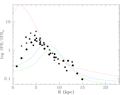
Figure 10: The radial profile of the SFR, normalized to its value at R_⊙=8 kpc and at the present time obtained with an exponential infall law as in eq. (7). The model curves are compared with the observations by Lacey & Fall (1985)–filled squares–, Gusten & Mezger (1983)–filled triangles– and Williams & McKee (1997)–filled circles. The model curves are at 1 (dotted-dashed line), 5 (dotted line), 8 (dashed line) Gyr from the formation of the Galaxy, and the present time (continuous line).

A.2 The parameters of the model

The mass fractions in each component computed by the model in each annulus are then converted into surface densities using as a normalization the observed total baryonic surface density (i.e. the sum of the Hi, H₂, stellar and remnant surface densities). The observed gas surface density is taken from Dame et al. (dame93 (1993)), and the stellar surface density, including remnants, from Boissier & Prantzos (boissier99 (1999)), with an exponential scale-length of 2.5 kpc (Ruphy et al. ruphy96 (1996)) and a normalization value at the solar radius of $43\pm 5$ $M_{\odot}$ pc^-2 (Mera et al. mera98 (1998)). In the comparison with the data, we identify the diffuse gas and cloud components with the Hi and the H₂ gas, respectively.

For our model of the Galaxy we adopt the “best” values of the various coefficients (infall, cloud and star formation efficiencies) in the solar neighborhood, scaling them at different Galactocentric radii, as discussed by Ferrini et al. (ferrini94 (1994)), Mollà et al. (molla96 (1996)), Mollà & Diaz (molla05 (2005)), Magrini et al. (magrini07 (2007)). The efficiencies of the processes regulating the conversion of diffuse gas into clouds and clouds into stars are close to those found in the best model for the Galaxy of Mollà & Diaz (molla05 (2005)), corresponding to the efficiencies of their morphological type $N=4$ (see their Table 2). In Table 4 we show the values of the coefficients we have adopted for our best model. $R_{D}$ and $R_{H}$ are the scale heights of the disk (cf. Sackett sackett97 (1997)) and of the halo (cf. Boissier & Prantzos boissier99 (1999)), respectively. $\lambda_{D}$ is a typical disk scale length (cf. Ferrini et al. ferrini94 (1994), Portinari & Chiosi portinari99 (1999)). $\mu$ is the efficiency of the cloud formation from diffuse gas, $H$ that of the star formation from cloud collisions, and $H^{\prime}$ that of cloud dispersion.

	$h_{D}$	$R_{H}$	$\lambda_{D}$	$H(R_{\odot}$)	$H^{\prime}(R_{\odot}$)	$\mu(R_{\odot}$)	$f_{0}$
	(kpc)	(kpc)	(kpc)	(107  yr)-1	(107 yr)-1	(107  yr) -1	(107  yr)-1
MW	0.3	35	2.0	0.20	1.0	0.09	0.012

Table 4: Parameters of the GCE models for the MW. $R_{D}$ and $R_{H}$ are the scale heights of the disk and of the halo, respectively. $\lambda_{D}$ is the scale length of the infall. $H$ (star formation efficiency from cloud collisions), $H^{\prime}$ (cloud dispersion) and $\mu$ (cloud formation), and $f$ (infall) are given at the solar radius ($R_{\odot}$).

The chemical enrichment of the gas is modeled using the matrix formalism developed by Talbot & Arnett (talbot73 (1973)). The elements of the restitution matrices $Q_{i,j}(M,Z)$ are defined as the fraction of the mass of an element $j$ initially present in a star of mass $M$ and metallicity $Z$ that it is converted into an element $i$ and ejected. Our GCE model takes into account two different metallicities, $Z=0.02$ and $Z=0.006$, and 22 stellar mass bins (21 for $Z=0.006$) from $M_{\rm min}=0.8$ $M_{\odot}$ to $M_{\rm max}=100\leavevmode\nobreak\$ $M_{\odot}$, for a total of 43 restitution matrices. For low- and intermediate-mass stars ($M<8$ $M_{\odot}$) we use the yields by Gavilán et al. (gavilan05 (2005)) for both values of the metallicity. For stars in the mass range $8\leavevmode\nobreak\ M_{\odot}<M<35\leavevmode\nobreak\ M_{\odot}$ we adopt the yields by Chieffi & Limongi (chieffi04 (2004)) for $Z=0.006$ and $Z=0.02$.

We estimate the yields of stars in the mass range $35\leavevmode\nobreak\ M_{\odot}<M<100\leavevmode\nobreak\ M_{\odot}$, which are not included in tables of Chieffi & Limongi (chieffi04 (2004)) by linear extrapolation of the yields in the mass range $8\leavevmode\nobreak\ M_{\odot}<M<35\leavevmode\nobreak\ M_{\odot}$. In the case of Ti, we increased the yields by a factor of 2 to reproduce the observations. The SNIa yields are taken from the model CDD1 by Iwamoto et al. (iwamoto99 (1999)).

Another fundamental ingredient of a GCE model is the initial mass function (IMF). Several parameterizations of the IMF have been widely used in the literature. Since the magnitude and the slope of the modeled chemical abundance gradients are related to the choice of the IMF, we checked the consistency of several IMFs with the observed gradients. With the adopted infall, efficiencies and set of chemical yields, we have found the best agreement with the observed gradients using the IMF by Kroupa et al. (kroupa93 (1993)).

A.3 Results of the model

A successful chemical evolution model of the Milky Way should reproduce the observed radial profiles and the integrated quantities. Fundamental radial profiles to be reproduced are: i) the gas radial distribution (e.g. Dame dame93 (1993)); ii) the stellar exponentially decreasing profile; iii) the strongly decreasing SFR profile; iv) the metallicity gradients of various elements. The integrated quantities are instead the average infall rate, the average SFR, and the supernovae rates of both SNII and SNIa.

In Figures 11 and 12 we present the comparison of the results of our model with the previously described radial profiles. Note that the model describes only the evolution of the disk, thus the inner regions hosting the bulge are not expected to be reproduced (R$\lesssim$5 kpc). The radial profiles of the total gas and of the stars at the present time are well reproduced, as is the radial profile of O/H as drawn by H ii regions. Note however the large dispersion in the observations. The general trend of the SFR is reproduced by the model, even if the observed maximum is at $\sim$6-7 kpc, while the model maximum is located at $\sim$9-10 kpc

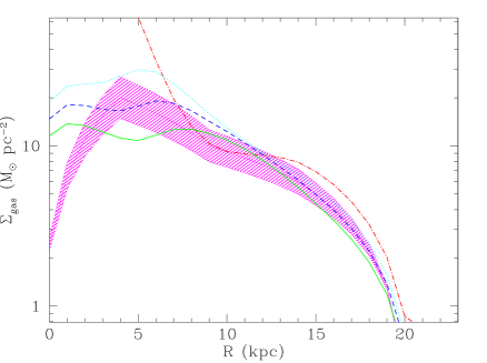
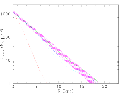
Figure 11: Results of the chemical evolution model for the Galactic disk and comparison to observations a) Total gas profile, model at 1, 5, 8 Gyr, and present time from the formation of the Galaxy, observations by Dame (dame93 (1993)); b) Stellar profile, model as in a), and observations by Mera et al. (mera98 (1998)), within two exponential disks of scale-lengths 2.2 and 2.6 kpc, respectively and normalized to the current local star surface density; line types for the model are as in Fig. 10.

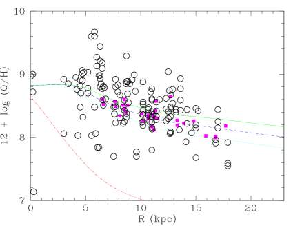
Figure 12: Results of the chemical evolution model for the Milky Way disk, model at different times as in Fig.11. a) Oxygen abundance gradient compared with the HII regions gradients by Deharveng et al. (deharveng00 (2000), filled squares) and Rudolph et al. (rudolph06 (2006)), empty circles). b) Radial profile of the infall of gas into the disk Line types for the model are as in Fig. 10.

Our “best” model is also able to reproduce the observational integrated quantities for the Galaxy, as: (i) the present-time infall rate is 3.5 $M_{\odot}$ yr^-1 integrated over 22 kpc radii, consistent with the recent estimate $\sim 5$ $M_{\odot}$ yr^-1 by de Boer (deboer04 (2004)), and favoured by recent models of disk galaxy evolution (e.g., Naab & Ostriker naab06 (2006)); (ii) the predicted current star formation rate is $\sim 3$ $M_{\odot}$ yr^-1 integrated over 22 kpc radii, to be compared with the observed value e.g. by Pagel (pagel97 (1997)) of 2-6 $M_{\odot}$ yr^-1; (iii) the current supernova rates obtained from the model are 1.6 SN/century for SNIa and 1.4 SN/century for SNII, of the same order as the values for Sb galaxies $\sim 1.8$ SN/century and $\sim 2$ SN/century, respectively (Mannucci et al. mannucci05 (2005)).

- (1) Andrievsky, S.M., Luck, R. E., Martin, P., Lèpine, J. R. D. 2004, A&A, 413, 159
- (2) Bedin, L.R., Piotto, G., Carraro, G., King, I.R., Anderson, J. 2006, A&A, 460L, 27
- (3) Boesgaard, A.M., Friel, E.D. 1990, ApJ, 351, 467
- (4) Boissier, S., Prantzos, N. 1999 MNRAS, 307, 857
- (5) Bragaglia, A., Tosi, M., 2006 AJ, 131, 1544
- (6) Bragaglia, A., Sestito, P., Villanova, S. et al. 2008 A&A, 480, 79
- (7) Carraro, G., Ng, Y.K., Portinari, L. 1998 MNRAS, 296, 1045
- (8) Carraro, G., Bresolin, F., Villanova, S., et al. 2004 AJ, 128, 1676
- (9) Carraro, G., Villanova, S., Demarque, P., et al. 2006 ApJ, 643, 1151
- (10) Carraro, G., Geisler, D., Villanova, S., Frinchaboy, P. M., Majewski, S. R. 2007 A&A, 476, 217
- (11) Carraro, G., Villanova, S., Demarque, P., Moni Bidin, C., McSwain, M.V. 2008 MNRAS, 386, 1625
- (12) Carretta, E., Bragaglia, A., Gratton, R., Tosi, M. 2004 A&A, 422, 951
- (13) Cescutti, G., Frano̧is, P., Matteucci, F., Cayrel, R., Spite, M. 2006 A&A, 448, 557
- (14) Chabrier, G. 2003 PASP, 115, 763
- (15) Chen, L., Hou, J. L., Wang, J. J. 2003 AJ, 125, 1397
- (16) Chiappini, C., Matteucci, F., Gratton, R. 1997 ApJ, 477, 765
- (17) Chiappini, C., Matteucci, F., Romano, D. 2001 ApJ, 554, 1044
- (18) Chieffi, A., Limongi, M. 2004 ApJ, 608, 405
- (19) Corder, S., Twarog, B.A. 2001 AJ, 122, 895
- (20) Dame, T., Holt, S., Verter, F., 1993 Back to the Galaxy, 267 Am. Inst. Phys., New York
- (21) de Boer, K. S. 2004 A&A, 419, 527
- (22) Deharveng, L., Pena, M., Caplan, J., Costero, R., 2000 MNRAS, 311, 329
- (23) Ferrini, F., Penco, U., Palla, F. 1990 A&A, 231, 391
- (24) Ferrini, F., Matteucci, F., Pardi, C., Penco, U. 1992 ApJ, 387, 138
- (25) Ferrini, F., Mollà, M., Pardi, M. C., Diaz, A. I., 1994 ApJ, 427, 745
- (26) Ford, A., Jeffries, R. D., Smalley, B., 2005 MNRAS, 364, 272
- (27) François, P., Matteucci, F., Cayrel, R., Spite, M., Spite, F., Chiappini, C., 2004 A&A, 421, 613
- (28) Friedli, D. 1998, ASPC, 147, 287
- (29) Friel, E. D., Janes, K.A. 1993, A&A, 267, 75
- (30) Friel, E. D. 1995, ARA&A, 33, 381
- (31) Friel, E. D., Janes, K.A., Tavarez, M., et al. 2002, AJ, 124, 2693
- (32) Friel, E. D., Jacobson, H.R., Barrett, E., et al. 2003, AJ, 126, 2372
- (33) Friel, E. D., Jacobson, H.R., & Pilachowski, C.A. 2005, AJ, 129, 272
- (34) Friel, E. D. 2006, in “Chemical Abundances and Mixing in Stars in the Milky Way and its Satellites”, eds. S. Randich & L. Pasquini, ESO Astrophysic Symposia, Vol. 24, Springer-Verlag, p. 3
- (35) Gavilán, M., Buell, J. F., Mollà, M. 2005, A&A, 432, 861
- (36) Giovagnoli, A., & Tosi, M. 1995, MNRAS, 273, 499
- (37) Goetz, M., Koeppen, J. 1992, A&A, 262, 455
- (38) Gonzalez, G., Wallerstein, G. 2000, PASP, 112, 1081
- (39) Gratton, R. G., Contarini, G. 1994, A&A, 283, 911
- (40) Hamdani, S., North, P., Mowlavi, N., Raboud, D., Mermilliod, J.-C. 2000, A&A, 360, 509
- (41) Henry, R. B. C., Worthey, G. 1999, PASP, 111, 919
- (42) Hou, J. L., Prantzos, N., Boissier, S. 2000, A&A, 362, 921
- (43) Koeppen, J. 1994, A&A, 281, 26
- (44) Kroupa, P., Tout, C. A., Gilmore, G. 1993, MNRAS, 262, 545
- (45) Jacobson, H. R., Friel, E. D., Pilachowski, C. A. 2008, AJ, 135, 2341
- (46) Janes, K. A. 1979, ApJS, 39, 135
- (47) Iwamoto, K., Brachwitz, F., Nomoto, K., et al. 1999, ApJS, 125, 439
- (48) Lacey, C. G., & Fall, S. M. 1985, ApJ, 290, 154
- (49) Lemasle, B., Frano̧is, P., Bono, et al. 2007, A&A, 467, 283
- (50) Maciel, W. J. 2000 NewAR, 45, 57
- (51) Maciel, W. J., Costa, R. D. D., Uchida, M. M. M. 2003, A&A, 397, 667
- (52) Maciel, W. J.; Quireza, C.; Costa, R. D. D. 2007, A&A, 463, 13
- (53) Maciel, W. J., & Costa, R. D. D. 2008, arXiv:0806.3443
- (54) Maeder, A., Meynet, G. 1989, A&A, 210, 155
- (55) Magrini, L., Corbelli, E., Galli, D. 2007, A&A, 470, 843
- (56) Mannucci, F., Della Valle, M., Panagia, et al. 2005, A&A, 433, 807
- (57) Manzi, S., Randich, S., de Wit, W.-J., Palla, F. 2008, A&A, 479, 141
- (58) Matteucci, F., Chiappini, C. 2005, PASA, Volume 22, Issue 1, p. 49.
- (59) Mera, D., Chabrier, G., Schaeffer, R. 1998, A&A, 330, 953
- (60) Mollà, M., Ferrini, F., Diaz, A. I. 1996, ApJ, 466, 668
- (61) Mollà, M., Ferrini, F., Diaz, A. I. 1997, ApJ, 475, 519
- (62) Mollà, M., Diaz, A. I. 2005, MNRAS, 358, 521
- (63) Naab, T., Ostriker, J.P. 2006, MNRAS, 366, 899
- (64) Pace, G., Pasquini, L., François, P. 2008, A&A, 489, 403
- (65) Pagel, B. E. J. 1997, Nucleosynthesis and Chemical Evolution of Galaxies, Cambridge Univ. Press, Cambridge
- (66) Pasquini, L., Randich, S., Zoccali, M., et al. 2004, A&A, 424, 951
- (67) Paulson, D. B., Sneden, C., Cochran, W. D. 2003, AJ, 125, 3185
- (68) Perinotto, M., Morbidelli, L. 2006, MNRAS, 372, 45
- (69) Phelps, R. L., Janes, K. A., Montgomery, K. A. 1994, AJ, 107, 1079
- (70) Phelps, R. L., Janes, K.A. 1996, AJ, 111, 1604
- (71) Portinari, L., Chiosi, C. 1999 A&A, 350, 827
- (72) Portinari, L., Chiosi, C. 2000, A&A,355, 929
- (73) Pottasch, S. R., & Bernard-Salas, J. 2006, A&A, 457, 189
- (74) Randich, S., Sestito, P., Primas, F., Pallavicini, R., Pasquini, L. 2006, A&A, 450, 557
- (75) Reddy, B. E., Lambert, D. L., Allende Prieto, C. 2006, MNRAS, 367, 1329
- (76) Robichon, N., Arenou, F., Mermilliod, J.-C., Turon, C. 1999, A&A, 345, 471
- (77) Rudolph, A. L., Fich, M., Bell, G. R., Norsen, T., Simpson, J. P., Haas, M. R., Erickson, E. F. 2006, ApJS, 162, 346
- (78) Ruphy, S., Robin, A. C., Epchtein, N., et al. 1996 A&A, 313, 21
- (79) Sackett, P. 1997, ApJ, 483, 103.
- (80) Salaris, M., Weiss, A., Percival, S. M. 2004, A&A, 414, 163
- (81) Salpeter, E. E. 1955, ApJ, 121, 161
- (82) Scalo, J. 1986, Fundamentals of Cosmic Physics, 11, 1
- (83) Scalo, J. 1998, ASPC, 142, 201
- (84) Schuler, S. C., King, J. R., Fischer, D. A., Soderblom, D. R., Jones, B. F. 2003, AJ, 125, 2085
- (85) Sestito, P., Randich, S., Mermilliod, J.-C., Pallavicini, R. 2003, A&A, 407, 289
- (86) Sestito, P., Bragaglia, A., Randich, S., Carretta, E., Prisinzano, L., & Tosi, M. 2006, A&A, 458, 121
- (87) Sestito, P., Randich, S., Bragaglia, A. 2007, A&A, 465, 185
- (88) Sestito, P., Randich, S., Bragaglia, A., Pallavicini, R., Andrievsky, S. M. 2008, A&A, in press, arXiv0807.2313
- (89) Shen, Z.-H., Jones, B., Lin, D.N.C., Liu, X.-W., Li, S.-L. 2005, ApJ, 635, 608
- (90) Stanghellini, L., Guerrero, M. A., Cunha, K., Manchado, A., Villaver, E. 2006, ApJ, 651, 898
- (91) Talbot, R. J., Jr., Arnett, W. D. 1973 ApJ, 186, 51
- (92) Tautvaisien G., Edvardsson, B., Puzeras, E., Ilyin, I. 2005, A&A, 431, 933
- (93) Tinsley, B. M. 1981, Fundamentals of Cosmic Physics, 5, 287
- (94) Tosi, M. 1988, A&A, 197, 33
- (95) Tosi, M. 1996, ASP Conf. Ser. 98, 299
- (96) Twarog, B. A., Ashman, K. M., Anthony-Twarog, B. J. 1997, AJ, 114, 2556
- (97) Villanova, S., Carraro, G., Bresolin, F., Patat, F. 2005, AJ, 130, 652
- (98) Yong, D., Carney, B. W., de Almeida, L. 2005, AJ, 130, 597