Generic susceptibilities of the half-filled Hubbard model in infinite dimensions

Abstract

Around a metal-to-insulator transition driven by repulsive interaction (Mott transition) the single particle excitations and the collective excitations are equally important. Here we present results for the generic susceptibilities at zero temperature in the half-filled Hubbard model in infinite dimensions. Profiting from the high resolution of dynamic density-matrix renormalization at all energies, results for the charge, spin and Cooper-pair susceptibilities in the metallic and the insulating phase are computed. In the insulating phase, an almost saturated local magnetic moment appears. In the metallic phase a pronounced low-energy peak is found in the spin response. It is the precursor of the magnetic moment in the insulator.

I Introduction

Strongly correlated systems persist to be a very interesting field of current research. In particular in the vicinity of a quantum phase transition the physics is very rich because the nature of the ground state and of the excitations changes. One prominent example of such a phase transition at zero temperature is the metal-to-insulator transition driven by an increasing local repulsive interaction: the so-called Mott transition. For low values of the interaction the system is metallic because the electrons can still pass one another. For large values of the repulsive Coulomb interaction, there can be at most one electron per site. If the system is exactly half-filled, each site is occupied by one electron. No motion of electrons is possible because they are blocking one another. Hence the system is insulating.

The simplest model describing the Mott transition is the Hubbard model. Hubbard (1963); Kanamori (1963); Gutzwiller (1963) The one-dimensional case can be solved analytically and has been studied intensively.Essler et al. (2005) It is governed by the particular phenomena of one-dimensional physics such as spin-charge separation. Yet this is not the generic physics occurring in higher dimensions. Very much of our current understanding of the Mott transition in higher dimensions is based on the limit of infinite dimensionsMetzner and Vollhardt (1989); Müller-Hartmann (1989) which leads to the dynamic mean-field theory (DMFT) (Refs. Pruschke et al., 1995 and Georges et al., 1996) as important approximation scheme for real narrow-band compounds.

The essential result of DMFT is that the transition between metal and paramagnetic insulator is marginally first order.Georges et al. (1996); Bulla (1999); Bulla et al. (2001); Blümer (2002); Potthoff (2003); Karski et al. (2005) It is first order at finite temperature where a finite amount of spectral weight is redistributed at the transition $U_{c}$ with $U_{c1}(T)<U_{c}(T)<U_{c2}(T)$. But at zero temperature only an infinitesimal amount of spectral weight is redistributed at $U_{c}(T=0)=U_{c2}(T=0)$ (Ref. Karski et al., 2005) so that the transition is continuous. The first order jump has just vanished. The insulator represents a metastable phase for $U<U_{c2}$ (Refs. Blümer, 2002 and Karski et al., 2005) (see Fig. 1).

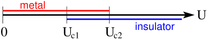
Figure 1: (color online) Phase diagram of the Mott transition of a half-filled Hubbard model in infinite dimensions with semi-elliptic density-of-states at zero temperature as function of the interaction $U$. The critical value below which the insulator ceases to exist is $U_{c1}=2.38\pm 0.02D$. The critical value above which the metal ceases to exist is $U_{c2}=3.07\pm 0.1D$ (Refs. Karski et al., 2005 and Karski et al., 2008). But between $U_{c1}$ and $U_{c2}$ the metal has the lower energy so that the insulator is only metastable (Ref. Karski et al., 2005).

Historically, there are two scenarios for the Mott transition based on opposite limits. The Brinkmann-Rice scenario captures the essential point on the metallic side, namely the band-narrowing.Brinkman and Rice (1970) The Hubbard scenario captures the two bands in the insulator (Hubbard bands), which approach each other till they touch at the point where the insulator becomes unstable.Hubbard (1964) The DMFT combines the strong points of both preceding scenarios.Zhang et al. (1993); Georges et al. (1996); Bulla (1999); Kotliar (1999); Bulla et al. (2001); Karski et al. (2005, 2008) Already the metallic solution displays Hubbard bands. The difference between the metallic and the insulating solution is found in the re-distribution of spectral weight at moderate energies only while the spectral densities at higher energies coincide. This coincidence is quantitative for $U\to U_{c2}$ as shown in Ref. Karski et al., 2005.

So the generic single-particle dynamics as encoded in the single-particle propagator is by now well-understood for the Mott transition. The dynamics of collective excitations and in particular the interplay between the single-particle modes and the collective modes is less well understood and investigations are ongoing.Byczuk et al. (2007); Raas et al. (2008)

A truly open issue is the physical origin of sharp features found at the inner band edges of the Hubbard bands just before the system switches from metallic to insulating behavior. These features were observed in quite a number of investigations but they were discussed as physical phenomenon only recentlyKarski et al. (2005, 2008) based on high-resolution dynamic density-matrix renormalization (D-DMRG). The features are confirmed by independent D-DMRG calculationsNishimoto et al. (2006) and by high-resolution numerical renormalization (NRG) (Ref. Žitko and Pruschke, 2009) but called into question by quantum Monte-Carlo extrapolations.Blümer (2008)

For the above reasons we have performed a thorough investigation of the susceptibilities in the half-filled Hubbard model in infinite dimensions. The calculations start from the self-consistent solutions obtained by iterating the DMFT self-consistency cycle Georges and Kotliar (1992); Jarrell (1992); Georges et al. (1996) with D-DMRG as impurity solver.Karski et al. (2005, 2008) We benefit again from the good control of the energy resolution achievable by D-DMRG for all energies.

The susceptibilities provide valuable complementary information to the single-particle propagator. They address bosonic observables such as the local charge or spin or Cooper-pair density and their dynamics. So they give information about the corresponding collective modes. Moreover, the susceptibilities are experimentally relevant. The charge susceptibility corresponds to the polarizability which determines the response seen in linear optics such as in infrared absorption. The spin susceptibility can be measured by inelastic neutron scattering. For these reasons, the susceptibilities $\chi^{\text{charge}}$, $\chi^{\text{spin}}$, and $\chi^{\text{pair}}$ are addressed in the present article.

The paper is organized as follows. In Sec. II, we introduce the model. In Sec. III, the susceptibilities will be defined in detail. Analytic statements about them will be derived there. The numerical results in the insulating and in the metallic phases will be given and their physical implications will be discussed. The conclusions summarize the article.

II Model and Method

We study the Hubbard model in DMFT at half-filling. The Hamiltonian reads

$$\mathcal{H}=-t\sum_{\langle i,j\rangle;\sigma}c^{\dagger}_{i;\sigma}c^{\phantom{\dagger}}_{j;\sigma}+U\sum_{i}(\hat{n}_{i;\uparrow}-1/2)(\hat{n}_{i;\downarrow}-1/2).$$ (1)

Here $c^{\dagger}_{i;\sigma}$ creates a fermion of spin $\sigma$ at site $i$ while $c_{i;\sigma}$ annihilates such a fermion. The matrix element $t$ labels the hopping of the fermions from site to site, i.e., their kinetic energy. The matrix element $U>0$ labels the on-site Coulomb repulsion of two electrons on the same site. It is an effective parameter which takes the screening into account.

We assume that the lattice on which it is defined is bipartite so that the Hamiltonian (1) displays particle-hole symmetry. In our physical discussion we will assume that the system is translationally invariant so that the momentum dependence of a propagator can be considered. The actual calculations, however, will be done for a non-interacting semi-elliptic density-of-states (DOS)

$$\rho_{0}(\omega)=(2/(\pi D^{2}))\sqrt{D^{2}-\omega^{2}}$$ (2)

which is characteristic for the Bethe lattice with infinite branching ratio.Economou (1979) The advantage of this approach is calculational simplicity and a finite support in contrast to the Gaussian tails on truly hypercubic lattices.Metzner and Vollhardt (1989); Müller-Hartmann (1989)

The limit of infinite dimensions $d$ or equivalently of an infinite coordination number $z$ exists if $t$ is scaled like $t^{\star}/\sqrt{z}$. This limit defines the DMFT.Metzner and Vollhardt (1989); Müller-Hartmann (1989); Georges and Kotliar (1992); Jarrell (1992); Georges et al. (1996) The self-energy $\Sigma_{ij}$ becomes local $\Sigma_{ij}=\delta_{ij}\Sigma_{ii}$ and equals the self-energy of a single-impurity Anderson modelHewson (1993) which has the same skeleton diagrams in all orders. This means that the local dressed propagator $G_{ii}$ must be the same which defines the self-consistency condition of the DMFT. The ensuing simplification is that one only has to solve a zero-dimensional problem: an interacting site coupled to a bath. One way to represent this bath is as semi-infinite chain so that the problem is amenable to powerful one-dimensional tools, for instance dynamic DMRGGarcia et al. (2004); Karski et al. (2005) which ensures a good control of the energy resolution over all energies.Raas et al. (2004) For details, we refer the reader to Ref. Karski et al., 2008.

III Susceptibilities

In a translationally invariant system it is appropriate to consider the momentum-dependent $\chi(\mathbf{q})$. But the implications of the limit of infinite dimensions are easier seen in real space. In real space $\chi$ depends only on the difference $\mathbf{r}_{i}-\mathbf{r}_{j}$ between the site $i$ where the observable is measured and the site $j$ where the field is applied. In the limit $d\to\infty$ each fermionic propagator from $i$ to $j$ is scaled by a factor $d^{-||i-j||/2}$ where $||\cdot||$ is the taxi cab or New York metric which counts the minimum number of hops required to get from $i$ to $j$. In a diagrammatic description of the propagation of any bosonic, collective observable from $i$ to $j$ at least two fermionic propagators link $i$ and $j$. This implies that such a susceptibility is suppressed by $d^{-||i-j||}$. Hence only local susceptibilities from $i$ to $i$ matter in infinite dimensions, at least in the absence of phase transitions.

This conclusion is not quite the whole story because certain non-local contributions can add up. For instance there are $2d$ next-neighbor contributions ($||i-j||=1$) to $i$ so that they make a non-negligible contribution if they add up since $2d/d=2$. But they will not add up for a generic momentum $\mathbf{q}$. The momentum $\mathbf{q}$ enters the susceptibilities only via

$$\eta(\mathbf{q})=\frac{1}{d}\sum_{p=1}^{d}\cos(q_{p})$$ (3)

where $q_{p}$ is the component in direction $p$.Müller-Hartmann (1989); Uhrig and Vlaming (1993) In the limit $d\to\infty$ almost all vectors $\mathbf{q}$ imply $\eta(\mathbf{q})=0$ since $\sqrt{d}\eta(\mathbf{q})$ is gaussian distributed with finite variance. Only particular values of measure zero, for instance $\mathbf{q}=(\pi,\pi,\pi,\ldots,\pi)^{\dagger}$, imply a non-vanishing $\eta$. Hence, the generic susceptibility is the one for $\eta=0$ which corresponds in real space to the local one.

Of course, some important effects of finite-dimensional physics are not captured by the generic susceptibilities. For example an antiferromagnetic instability or the instability to an incommensurate phase is indicated by the divergence of a susceptibility for some $\eta\neq 0$. This must be kept in mind. On the other hand, however, the propagation of collective modes as they interact with single particles is given in $d=\infty$ by the generic susceptibilities. In any diagram for the proper self-energy which contains the propagation of a collective mode there is also a sum over its momentum. Hence the peculiar contributions with $\eta\neq 0$ do not matter here. It is the generic behavior of collective modes at $\eta=0$ which is relevant for the interaction with single particles in $d=\infty$.

Note that this argument remains true even if the DMFT is not seen as the limit of infinite dimensions but more broadly as a consistent local approximation scheme. This is by now a very common view adopted in the description of real compounds. Then one can discuss the whole momentum dependence of the susceptibility. But the behavior of the collective modes which enters implicitly in the description of the single-particle dynamics remains the one given by the local susceptibilities. For this reason, we compute and discuss the local susceptibilities in the following.

The local susceptibilities are easily accessible since they are identical to the local susceptibilities at the interaction site of the auxiliary single-impurity Anderson model. This is obvious if one thinks of the susceptibilites as being given by an expansion in terms of skeleton diagrams to infinite order.

In the sequel, we will present the imaginary parts of the susceptibilities since these parts provide direct information on the energies and spectral weights of collective excitations.

One drawback of the susceptibilities is that their imaginary parts are antisymmetric (odd) by construction $\text{Im}\chi(\omega)=-\text{Im}\chi(-\omega)$. Hence the very interesting behavior at zero and at very low energies is suppressed. For instance, let $Q$ be an hermitean bosonic observable like the spin density. With $|0\rangle$ being the ground state and $E_{0}$ its energy, the matrix element of the resolvent

$$R(\omega):=\left\langle 0\big{|}Q(\omega-(\mathcal{H}-E_{0}))^{-1}Q\big{|}0\right\rangle$$ (4)

can have a $\delta$ peak at $\omega=0$ in its imaginay part. This would constitute an important piece of information on the system. But the susceptibility $\chi$ constructed from $R$ according to

$$\chi(\omega)=-R(\omega+i0+)-R(-\omega-i0+)$$ (5)

would not display this $\delta$ peak because it cancels on the right hand side of (5). In order not to lose the information at zero and at very low frequencies we will display results for

$$\text{Im}\chi_{+}(\omega)=\text{Im}R(\omega)$$ (6)

which is the contribution for non-negative frequencies. The contribution for negative frequencies is implied by antisymmetry, i.e., $\text{Im}\chi_{-}(\omega)=-\text{Im}\chi_{+}(-\omega)$.

An important tool in understanding spectral densities are sum rules. From the relation (6), the definition (4), and the Hilbert representation of $R(\omega)$ it is obvious that the total spectral weight takes the value

$$\int_{0}^{\infty}\chi_{+}(\omega)d\omega = \pi\lim_{\omega\to\infty}\omega R(\omega)$$ (7a)

$$= \pi\left\langle 0\big{|}Q^{2}\big{|}0\right\rangle.$$ (7b)

So knowing the ground state expectation value of $Q^{2}$ helps to understand general trends in spectral weights and it provides an important check for numerical calculations

A last important point concerns the computation of spectral densities like $\text{Im}\chi_{+}(\omega)$ by D-DMRG. The dynamic DMRG calculates a correction vector $|\text{cv}\rangle$ besides the ground state $|0\rangle$ and the state obtained from the application of $Q$, $Q|0\rangle$.Ramasesha et al. (1997); Kühner and Monien (1998) This correction vector reads

$$|\text{cv}\rangle=(\omega+i\delta-(H-E_{0}))^{-1}Q|0\rangle.$$ (8)

Obviously, $\langle 0|Q|\text{cv}\rangle$ yields $R(\omega+i\delta)$. The computation of the correction vector requires a numerically demanding matrix inversion.Raas et al. (2004) If there is an inaccuracy $\varepsilon$ in the correction vector $|\text{cv}\rangle$ the imaginary part of $R(\omega+i\delta)$ can be obtained from a variational functional with a decreased inaccuracy of the order of $|\varepsilon|^{2}$, see Ref. Jeckelmann, 2002.

In any case, the numerical approaches require the imaginary frequency $\delta$ in (8) to be finite. This implies a certain broadening of the actual spectral density. In order to retrieve the unbroadened spectral density $\text{Im}\chi_{+}(\omega)$ we employ the non-linear least-bias (LB) deconvolution technique.Raas and Uhrig (2005) This approach yields always non-negative results as is to be expected for $\text{Im}\chi_{+}(\omega)$. For details of the approach we refer the reader to Ref. Raas and Uhrig, 2005. Any deviations from the procedure described therein will be given below where applicable.

III.1 Cooper Pair Susceptibility

Here we consider the local observable

$$Q^{\text{pair}}=c^{\dagger}_{i;\uparrow}c^{\dagger}_{i;\downarrow}+c^{\phantom{\dagger}}_{i;\downarrow}c^{\phantom{\dagger}}_{i;\uparrow}$$ (9)

which creates or annihilates a Cooper pair on site $i$. Of course, one would expect that the corresponding susceptibility $\chi^{\text{pair}}(\omega)$ is strongly suppressed in a Hubbard band with repulsive interaction. Yet it can contain interesting features, for instance at higher energy.

But it is not necessary to compute $\chi^{\text{pair}}(\omega)$ separately. Indeed, there is an underlying symmetry which links $Q^{\text{pair}}$ to $Q^{\text{charge}}$, see Eq. (12) below. As a result the pair susceptibility is identical to the charge susceptibility. So we will not discuss $\chi^{\text{pair}}(\omega)$ here but refer to the next subsection where $\chi^{\text{charge}}(\omega)$ is investigated.

The symmetry becomes apparent under the transformation $c^{\dagger}_{\sigma}\to\gamma^{\dagger}_{\sigma}$ according to

$$\gamma^{\dagger}_{\uparrow} := c^{\dagger}_{\uparrow}\cos\varphi-c^{\phantom{\dagger}}_{\downarrow}\sin\varphi$$ (10a)

$$\gamma^{\dagger}_{\downarrow} := c^{\dagger}_{\downarrow}\cos\varphi+c^{\phantom{\dagger}}_{\uparrow}\sin\varphi.$$ (10b)

On a bipartite lattice this transformation is performed on all even sites with the angle $\varphi$ and on all odd sites with the angle $-\varphi$. Then the hopping terms in (1) are left invariant, independent of the value of $\varphi$. The same is true for the onsite interaction as given by the term proportional to $U$ in (1). So the total Hamiltonian (1) remains invariant under (10).

The interesting relation is the one for the observables

$$Q^{\text{charge}}_{c}=Q^{\text{charge}}_{\gamma}\cos(2\varphi)+Q^{\text{pair}}_{\gamma}\sin(2\varphi)$$ (11)

where we use $Q^{\text{charge}}$ in anticipation of Eq. (12). The subscript _c refers to the expression in terms of the original fermions $c$ and $c^{\dagger}$ while the subscript _γ refers to the expression in terms of the transformed fermions $\gamma$ and $\gamma^{\dagger}$. Here the value of the angle of rotation $\varphi$ matters. For $\varphi=\pi/4$ we switch from the charge observable to the pair observable. Hence the corresponding local susceptibilities are indeed the same. No additional numerics is needed in the bipartite half-filled case.

The above symmetry transformation has not gone unnoticed. It is one of the transformations at the basis of the SO(5) theory which is comprehensively reviewed in Ref. Demler et al., 2004. One further important conclusion is that charge and superconducting order are degenerate as far as they stem from a bipartite Hubbard model at half-filling, for instance with negative $U$.

III.2 Charge Susceptibility

Here we consider the local observable

$$Q^{\text{charge}}=c^{\dagger}_{i;\uparrow}c^{\phantom{\dagger}}_{i;\uparrow}+c^{\dagger}_{i;\downarrow}c^{\phantom{\dagger}}_{i;\downarrow}-1$$ (12)

which measures the charge fluctuations around half-filling, i.e., the deviation of the total fermion number per site from $1$.

The general sum rule (7) requires the expectation value $\left\langle 0\big{|}Q^{2}\big{|}0\right\rangle$ which amounts for $Q^{\text{charge}}$ up to twice the double occupancy value. First we note

$$(Q^{\text{charge}})^{2}=2\hat{n}_{\uparrow}\hat{n}_{\downarrow}-(n_{\uparrow}+\hat{n}_{\downarrow})+1$$ (13)

where $\hat{n}_{\sigma}=c^{\dagger}_{i;\sigma}c^{\phantom{\dagger}}_{i;\sigma}$. This implies at half-filling

$$\int_{0}^{\infty}\chi_{+}^{\text{charge}}(\omega)d\omega=2\pi\left\langle 0\big{|}\hat{n}_{\uparrow}\hat{n}_{\downarrow}\big{|}0\right\rangle.$$ (14)

So the static quantity to be known for the sum rule is the double occupancy (see Refs. Nishimoto et al., 2004 and Karski et al., 2005).

III.2.1 Insulator

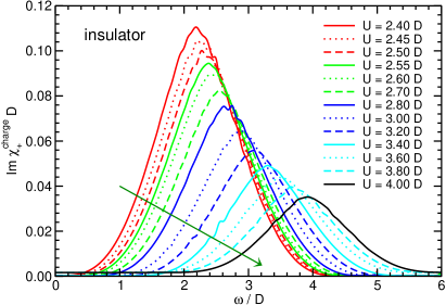
Figure 2: (color online) Positive imaginary part $\chi^{\text{charge}}_{+}$ of the local charge susceptibility in the insulating phase as function of frequency for various values of the interaction $U$. The arrow points in the direction of increasing interaction.

In Fig. 2 a series of numerical results is shown for the positive imaginary part $\chi^{\text{charge}}_{+}$ of the local charge susceptibility in the insulating phase. In the D-DMRG we kept $m=128$ states in the truncated DMRG basis. The mesh of frequencies is given by the interval $\Delta\omega=0.05D$ and the imaginary broadening was $\delta=0.1D$. The LB deconvolutionRaas and Uhrig (2005) was perforemd with a tolerance constant of $1/A_{\text{LB}}=1/100$. The curves are not perfectly smooth but display some wiggles. This is due to the deconvolution procedure employed.

Physically, no special features are discernible. But two trends are clearly visible. First, the susceptibility is more and more suppressed as the interaction is increased. This results in an overall reduction of the area under the curves. It can be quantified by the sum rule (14). So it is natural that the spectral weight of the charge response decreases on increasing $U$ because the latter suppresses the double occupancy $\langle 0|\hat{n}_{\uparrow}\hat{n}_{\downarrow}|0\rangle$ more and more.Nishimoto et al. (2004); Karski et al. (2005) We have checked this sum rule numerically and found it to be fulfilled to within a relative error of $1.8\%$ on the deconvolved data in the interval $\omega\in[0,5.9D]$.

Second, the spectral weight is shifted to higher and higher frequencies on increasing interaction. This is seen in two features. One is the peak position which is shifted. Its shift corresponds to the shift of spectral weight in the single-particle propagators.Nishimoto et al. (2004); Karski et al. (2005, 2008) These shifts reflect the simple fact that the energy difference between the lower and the upper Hubbard band is given by about $U$. Hence it increases linearly with $U$.

The other feature is the onset of finite spectral density which increases also with $U$. Due to the LB deconvolutionRaas and Uhrig (2005) there is no region where the spectral density is strictly zero. But we have checked that the susceptibility data is perfectly consistent with the natural assumption that the onset of the $\text{Im}\chi^{\text{charge}}_{+}$ takes place at $2\Delta$ where $\Delta$ is the single-particle gap (for data, see Karski et al., 2005 and Karski et al., 2008). For this check we analyzed the susceptibility data by fitting a quadratic onset $\propto(\omega-\omega_{\text{onset}})^{2}$ plus higher order corrections to its continuum. The quadratic onset is to be expected from the square root onset of the single-particle bandsNishimoto et al. (2004); Karski et al. (2005) which is convolved with itself in the standard particle-hole bubble. Because the single-particle gap rises upon increasing $U$ the collective response is shifted to higher and higher energies.

The onset at $2\Delta$ reflects the fact that the collective mode is made from a particle and a hole. In the particle-hole symmetric case considered here both have the same gap $\Delta$ so that any collective continuum starts only at $2\Delta$. A lower onset, i.e., at lower energy, could arise only if binding transferred spectral weight to the frequency interval below $2\Delta$. No indication for such a binding is found here.

III.2.2 Metal

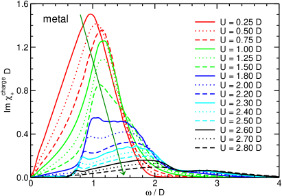
Figure 3: (color online) Positive imaginary part $\chi^{\text{charge}}_{+}$ of the local charge susceptibility as function of frequency for various values of the interaction $U$ in the metallic phase. The arrow points in the direction of increasing interaction. Note the different scale of the response compared to the response in the insulator in Fig. 2.

In Fig. 3 a series of numerical results is shown for the positive imaginary part $\chi^{\text{charge}}_{+}$ of the local charge susceptibility in the metallic phase. In the D-DMRG we kept between $m=128$ to $m=256$ states in the truncated DMRG basis; the frequency mesh is given by $\Delta\omega=0.05D$ and the imaginary broadening by $\delta=0.1D$. The LB deconvolutionRaas and Uhrig (2005) was performed with tolerance constants $1/A_{\text{LB}}=1/10$ and $1/A_{\text{LB}}=1/100$. The curves are not perfectly smooth but display some minor wiggles. This is due to the deconvolution procedure employed.

As in the insulating regime we find the trend that increasing interaction suppresses the charge response. This is expected because it is related to the same sum rule (14) which holds independent of the phase under study. Furthermore, the spectral response is shifted to higher and higher energy. Again this general trend can be related to the same trend in the single-particle propagators.Karski et al. (2005, 2008)

Interestingly, the charge response in the metallic phase displays much more structure than in the insulating phase. For low values of $U$ we find a linear increase with frequency $\omega$ for not too high values of $\omega\lessapprox 0.6D$. This is the expected behavior for a Fermi liquid. Its slope becomes smaller and smaller as the quasiparticles become heavier and heavier. From $U\approx 1.5D$ onwards, most of the charge response lies in an intermediate range $D\lessapprox\omega\lessapprox 2D$. There is still some spectral weight at lower frequencies but it is decreasing rapidly. An additional shoulder situated between $0.6D$ and $1D$ occurs above $U=1.8D$. We will discuss this feature in detail below. Above $U\approx 2.2D$ there is a third rather flat hump discernible centered around $\omega=3D$.

Qualitatively, the three regions of charge response can be understood from the single-particle response. The single-particle response, see for instance Figs. 12 and 13 in Ref. Karski et al., 2008, is mainly characterized by the heavy quasiparticle in the narrow central peak and by the broad emerging Hubbard bands of significant weight which are centered around $\omega\approx 1.5D$. Assuming that the collective response is roughly given by a single diagrammatic particle-hole bubble (or by an analytic function of this bubble as in the random phase approximation or in more sophisticated approaches such as the local moment approach),Logan et al. (1998); Galpin and Logan (2008) we simply have to convolve the single-particle response at positive frequencies with the one at negative frequencies.

The response at low frequencies $\omega\lessapprox 0.8D$ stems from the convolution of the central peak of heavy quasiparticles with itself. It dominates at low values of $U$, but on increasing $U$ it decreases in weight like $Z^{2}$ where $Z$ is the quasiparticle weight vanishing linearly for $U\to U_{c2}$. The quasiparticle weight $Z$ measures the spectral weight in the central peak.

The response at intermediate frequencies $0.8D\lessapprox\omega\lessapprox 2.2D$ stems from the convolution of the central peak of heavy quasiparticles with one of the Hubbard bands. Hence it is higher in frequency, because the Hubbard band is, and its weight decreases only linearly in $Z$

The response at higher frequencies results from the convolution of the lower and the upper Hubbard band. Hence it is located around twice their energy, i.e., around $3D$. This contribution is not suppressed by $Z$ so that it survives in the limit $U\to U_{c2}$. This is consistent with our data for $U=2.8D$ shown in Fig. 3. Unfortunately, no reliable data even closer to the critical value $U_{c2}$ could be obtained.

Note that only the last contribution at the higher frequency has an analog in the response in the insulator since there only the Hubbard bands exist. Indeed, the insulating response describes the high frequency metallic response very well as is illustrated in Fig. 4. The insulating and the metallic curve agree very well above $\omega\approx 3D$. The sizable differences below this frequency are remarkable in view of the shift of fairly little spectral weight between the metallic and the insulating single-particle solution.Karski et al. (2005) For experiment, for instance infrared absorption, Fig. 4 provides valuable information how different a metallic and an insulating system can look even though only tiny parameter changes are made. In the present case, even no parameters are changed, but only different hysteresis branches are considered.

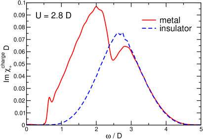
Figure 4: (color online) Positive imaginary part $\chi^{\text{charge}}_{+}$ of the local charge susceptibility as function of frequency for interaction $U=2.8D$ in the metallic and insulating phase.

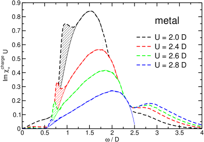
Figure 5: (color online) Positive imaginary part $\chi^{\text{charge}}_{+}$ of the local charge susceptibility as function of frequency for values of the interaction $U$ in the metallic phase, but close to the transition to the insulator. The main contribution is extrapolated as if there were no additional shoulder (thin solid lines). Then the shaded area is attributed to spectral weight of the shoulder.

Let us come back to the shoulder seen between $\omega\approx 0.6D$ and $\omega\approx 1D$ for $U\gtrapprox 1.8D$. Its position corresponds very precisely to the frequency where the sharp feature at the inner band edges has been found, see Fig. 2 in Ref. Karski et al., 2005 and Figs. 12 and 13 in Ref. Karski et al., 2008. Hence it is to be expected that there is a relation between both features. In view of the hypothesis that the sharp feature is caused by a resonance made from a heavy quasiparticle and a collective mode (see Refs. Karski et al., 2005 and Karski et al., 2008), it would be appealing to interprete the shoulder in Fig. 3 as the cause for the sharp feature in the single-particle spectral density. To pursue this idea further we plot in Fig. 5 the metallic charge response close to the transition to the insulator.

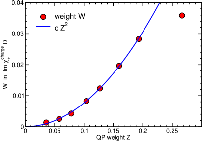
Figure 6: (color online) Spectral weight $W$ attributed to the shoulder in the metallic charge response as function of the quasiparticle weight $Z$. The solid line is a quadratic fit with $c=0.758$.

In the curves shown in Fig. 5 the shoulder is clearly visible. We extrapolate the main peak on which the shoulder sits smoothly. This is done by determining a frequency interval $[b_{1},b_{2}]$ below the shoulder and a second one $[b_{3},b_{4}]$ above it where the shoulder is not present. These intervals are found from analyzing minima and points of inflections of the original curve, for example for $U=2.4D$ we took $[0.56D,0.646D]$ and $[1.038D,2.175D]$. Then the data within these two intervals is interpolated by a 10${}^{\text{th}}$ order polynomial. This is taken to describe the continuum without the shoulder. The weight of the shoulder (shaded area in Fig. 5) is given by integrating the difference between the original curve with shoulder and the 10${}^{\text{th}}$ order polynomial in the interval $[b_{2},b_{3}]$. The resulting weights are well-defined within $4\cdot 10^{-4}$.

This procedure is applicable for the results obtained for $U/D\in\{2.0,2.2,2.3\ldots 2.7,2.8\}$. The resulting values are depicted in Fig. 6 as function of the quasiparticle weight $Z$. The quadratic fit agrees very well with the data except for the last point resulting from $U=2.0D$. For such a fairly low value of $U$ the separation of the shoulder from its background is not possible reliably.

Clearly, the shoulder weight $W$ depends quadratically on $Z$. We recall that the spectral weight $S$ of the sharp feature at the inner band edges in the single-particle propagator depends linearly on $Z$: $S\propto Z$ as found previously.Karski et al. (2005, 2008) These facts are incompatible with the sharp feature $S$ being the result of the shoulder $W$. It would require that right at the transition to the insulator the shoulder induces the sharp feature although the weight of the shoulder is infinitely smaller than the weight in the sharp peak.

But the other way around the quadratic behavior in Fig. 6 finds its natural explanation. The shoulder results from the convolution of the central quasiparticle peak of weight $Z$ with the sharp feature with $S\propto Z$. Hence $W\propto Z^{2}$ ensues as found.

Also the position in frequency is explained in this way. Since the central peak is located at zero frequency the shoulder as result of the convolution with the sharp feature is located at the frequency where the sharp feature is found.

Summarizing these findings, we conclude that the shoulder in the charge response can be understood as a consequence of the sharp feature at the inner band edges of the metallic single-particle spectral density. It is not its cause. While it is satisfying to have explained the origin of the shoulders in Figs. 5 and 6 we state that the physical origin of the sharp feature described in Refs. Karski et al., 2005 and Karski et al., 2008 is still unresolved.

III.3 Spin Susceptibility

Here we consider the local observable

$$Q^{\text{spin}}=c^{\dagger}_{i;\uparrow}c^{\phantom{\dagger}}_{i;\uparrow}-c^{\dagger}_{i;\downarrow}c^{\phantom{\dagger}}_{i;\downarrow}$$ (15)

which measures the spin fluctuations around zero magnetization in $z$ direction.

The general sum rule (7) requires the expectation value $\left\langle 0\big{|}Q^{2}\big{|}0\right\rangle$ which amounts for $Q^{\text{spin}}$ up to an expression which contains again the double occupancy. First we note

$$(Q^{\text{spin}})^{2}=\hat{n}_{\uparrow}+\hat{n}_{\downarrow}-2\hat{n}_{\uparrow}\hat{n}_{\downarrow}$$ (16)

where we used that the fermionic occupation number $\hat{n}$ is equal to its square. This implies at half-filling

$$\int_{0}^{\infty}\chi_{+}^{\text{spin}}(\omega)d\omega=\pi\left(1-2\left\langle 0\big{|}\hat{n}_{\uparrow}\hat{n}_{\downarrow}\big{|}0\right\rangle\right).$$ (17)

Note that this expression stays finite in the limit of vanishing double occupancy as it occurs for $U\to\infty$.

III.3.1 Insulator

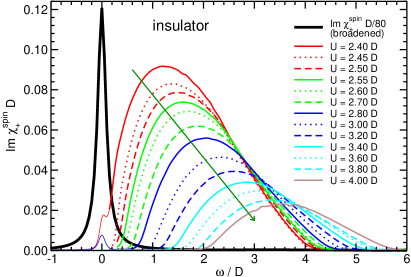
Figure 7: (color online) Positive imaginary part $\chi^{\text{spin}}_{+}$ of the local spin susceptibility in the insulating phase as function of frequency for various values of the interaction $U$. The arrow points in the direction of increasing interaction. The Lorentzian at zero frequency represents the example at $U=4D$ for the broadened $\delta$ peak occurring in the insulator.

In Fig. 7 a series of numerical results is shown for the positive imaginary part $\chi^{\text{spin}}_{+}$ of the local spin susceptibility in the insulating phase. In the D-DMRG we kept $m=128$ states in the truncated DMRG basis the mesh is given by the frequency interval $\Delta\omega=0.05D$, and the imaginary broadening is $\delta=0.1D$. In the LB deconvolution, the tolerance constant $A_{\text{LB}}=1/10$ is used.Raas and Uhrig (2005) The curves are not perfectly smooth but display some very small wiggles due to the LB deconvolution. The attempt to deconvolve the numerical DMRG data as a completely continuous spectral density leads to a very large and very narrow peak at low frequency (not shown). The continua beside this dominating term cannot be resolved reliably. But it turns out that the ansatz

$$\frac{1}{\pi}\text{Im}\chi_{+}^{\text{spin}}=A\delta(\omega)+\rho^{\text{cont}}(\omega)$$ (18)

works extremely well for deconvolution, see Fig. 7. Here $\rho^{\text{cont}}(\omega)$ stands for the continuous spectral density which is retrieved via the LB deconvolution. The weight $A$ of the $\delta$ peak results from the non-linear set of equations defining the Lagrange multipliers appearing in the LB ansatz.Raas and Uhrig (2005)

Why does a zero frequency $\delta$ function make sense physically in the local spin response of a paramagnetic insulator in infinite dimensions? The exchange coupling $J$ in a Heisenberg model derived from a Hubbard model in the insulating regime reads $J=4t^{2}/U$.Harris and Lange (1967) Hence scaling $t=t^{\star}/\sqrt{z}$ implies $J\propto 1/z$ and the exchange coupling does not contribute unless all the nearest neighbors contribute on average the same non-vanishing amount. This implies that a static mean-field treatment of the Heisenberg antiferromagnet around the Ising limit becomes exact in infinite dimensions.Kleine et al. (1995) There are no short-range spin-spin correlations. Hence each spin feels only the local field $h_{\text{MF}}=-zJm$ generated by the average magnetization $m$ of its $z$ neighbors. But in the paramagnetic phase which we consider here the average magnetization is zero: $m=0$. Hence there is no field and concomitantly there is no preferred direction of the local spin. This implies that the spin response is the one of a free spin, this means, a $\delta$ function at zero frequency. It signals that a local spin flip does not cost any energy.

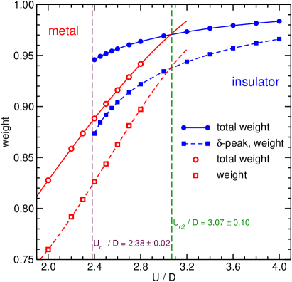
Figure 8: (color online) The total weight (circles) and four times the square of the local $S_{z}$ component (squares) of the spin response $\chi_{+}^{\text{spin}}(\omega)$ in the insulating (filled symbols) and in the metallic phase (open symbols). In the insulator the local $S_{z}$ component is taken from the weight $A$ of the $\delta$ peak as in Eq. (18). In the metal it is taken to be the weight of the dominant low energy peak, see Figs. 9 and 10. The dark lines interpolate the data in the insulator while the light lines interpolate and extrapolate the data in the metal.

Besides understanding this physics on the level of the infinite dimensional Hubbard model it can be understood on the level of the effective impurity model. Indeed, a gapped impurity model at particle-hole symmetry is found to be always in the so-called local moment regime,Chen and Jayaprakash (1998); Galpin and Logan (2008); Bulla et al. (2008) where a free local moment is formed.

The weight $A$ of the $\delta$ function represents four times the square of the local $S_{z}$ component in our normalization. It may not be confused with a static magnetization which is absent in the paramagnetic phase considered. For $U\to\infty$, $A$ takes the value unity since the spin $S=1/2$ is fully localized. At any finite interaction $U<\infty$, $A$ is reduced since charge fluctuations renormalize its value downward. The spins are not fully localized but smeared out to some extent to adjacent sites due to their virtual excursions. This behavior is analyzed quantitatively in Fig. 8 where the filled squares denote the values of $A$. Further discussion is presented below.

Besides the $\delta$ peak a continuous contribution of low weight persists. It correponds to the charge fluctuations which take some weight away from the dominant local spin response at zero frequency. Indeed, the continua are very similar, though not identical, to the ones found in the charge response in the insulating regime, see Fig. 2. To the accuracy that our numerical deconvolved data allows the onset of the continuous spectral spin response is again at $2\Delta$, i.e., twice the single-particle gap in the insulating regime. Hence the origin of the continuous spin response is essentially the excitation of particle-hole pairs. This is qualitatively similar to what one expects from the diagrammatic result in random-phase approximation where the response is a function of the particle-hole bubble.

The fact that most of the spectral weight in the spin response is found at zero frequency and not in the continuum starting at $2\Delta$ shows impressively that a binding phenomenon occurs. The spin response at zero frequency can be viewed as the signature of a bound state of a particle-hole pair. Only by binding one can understand how spectral weight can be transferred to energies lower than the sum of the energies of the constituent states. We think that such shift of spectral weight due to binding is not taken into account by the sophisticated argument on the spectral density close to the Mott transition.Kehrein (1998) This argument excluded the continuous scenario at zero temperature which is supported by most other analytical and numerical evidence (see Sec. I for a sketch of this scenario).

The total weight of the spin response as displayed in Fig. 8 just reflects the behavior of the double occupancy according to the sum rule (17). Hence it approaches unity for $U\to\infty$ but it does not become very small on $U\to U_{c1}$ either.

Much more interesting is the behavior of the square of the local $S_{z}$ component as quantified by $A$ in Eq. (18). The square root of this expression can be identified with the local magnetic moment. Clearly, $A=1$ at $U=\infty$ is the starting point. But it is remarkable that $A\approx 0.94$ has hardly decreased for $U=U_{c2}$ where the insulator is no longer the ground state. In physical terms this means that a Mott insulator is governed by very well localized spins as long as it exists. Hardly any renormalization due to charge fluctuations takes place. From a theoretical point of view this can be explained by the significant charge gap $\Delta\approx 0.45D$ at $U_{c2}$ (Ref. Karski et al., 2005) which acts as an infrared cutoff limiting the influence of charge fluctuations. This can be easily understood by the renormalization flow of the impurity model where the insulator corresponds to the local moment fixed point.Chen and Jayaprakash (1998); Bulla et al. (2008)

Even more remarkable is that the local magnetic moment is not much lower at $U_{c1}$ either. Below this interaction the insulator is not longer locally stable. Even there $A$ is still larger than about $0.87$ although the charge gap has become zero and the lower and the upper Hubbard band are touching each other, see for instance Fig. 2 in Ref. Karski et al., 2005. But it is obvious from the touching Hubbard bands that the DOS $\rho(\omega)$ at the Fermi level, i.e., at $\omega=0$, is still zero. We conclude that no hard infrared cutoff is needed and that the fact that the insulator at $U_{c1}$ displays a semi-metallic DOS with $\lim_{\omega\to 0}\rho(\omega)=0$ is sufficient to bound the influence of the charge fluctuations. So the magnetic moment is not renormalized to zero and the fixed point of the renormalization of the corresponding impurity model is still the local moment fixed point.Chen and Jayaprakash (1998); Bulla et al. (2008)

The main goal of this paper is the comprehensive analysis of the susceptibility around a Mott transition in infinite dimensions. But in view of the remarkable findings at $d=\infty$ it is in order to speculate how these findings change on passing to finite dimensional systems.

The main difference is that any finite dimensional system would show at least short-range magnetic correlations. Hence the magnetic response would not be governed by a $\delta$ peak at zero frequency as in Fig. 7. If the resulting antiferromagnetic system is sufficiently strongly frustrated and/or sufficiently low-dimensional so that the magnetic fluctuations are strong enough to prevent magnetic long-range order the system would be paramagnetic displaying a magnetic gap. Generically, the magnetic excitations would be triplonsSchmidt and Uhrig (2003) with some dispersion. Hence the local spin response would show the sum of triplon contributions from all the wave vectors in the Brillouin zone. A broad feature at finite frequencies in a frequency range given by the magnetic exchange $J$ would be seen in $\text{Im}\chi_{+}^{\text{spin}}(\omega)$. A sharp mode at finite, but low frequency would be discernible in $\text{Im}\chi_{+}^{\text{spin}}(\omega,\mathbf{q})$ at a given wave vector $\mathbf{q}$. The sum of the weights in these sharp modes over the Brillouin zone constitutes the finite dimensional analog of the weight $A$ in our infinite dimensional analysis. We expect other features to be qualitatively very similar to the above findings. For instance the local magnetic moment in any insulating state should be very little renormalized due to charge fluctuations.

III.3.2 Metal

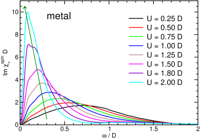
Figure 9: (color online) Positive imaginary part $\chi^{\text{spin}}_{+}$ of the local spin susceptibility in the metallic phase as function of frequency for various small values of the interaction $U$. The arrow points in the direction of increasing interaction. Note the quickly increasing peak at low frequencies and the quickly vanishing spectral weight at higher frequencies.

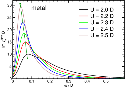
Figure 10: (color online) Positive imaginary part $\chi^{\text{spin}}_{+}$ of the local spin susceptibility in the metallic phase as function of frequency for various values of the interaction $U$ close to the transition to the insulator. The arrow points in the direction of increasing interaction. The peak at low frequencies prevails completely, note the scale on the $y$ axis.

In Fig. 9 a series of numerical results is shown for the positive imaginary part $\chi^{\text{spin}}_{+}$ of the local spin susceptibility in the metallic phase for not too large values of the interaction. The curves for larger values of $U$ are plotted in Fig. 10 In the D-DMRG we kept between $m=128$ and $m=256$ states in the truncated DMRG basis, the frequency mesh is given by the intervals $\Delta\omega=0.025D$ and $\Delta\omega=0.05D$, and the imaginary broadening is chosen between $\delta=0.05D$ and $\delta=0.1D$. The LB deconvolutionRaas and Uhrig (2005) is done with the tolerance constant $1/A_{\text{LB}}=1/10$.

As a first check of our data we compute the static spin spin susceptibility $\chi^{\text{spin}}(0)$ via the Kramers-Kronig relation

$$\chi^{\text{spin}}(0)=\frac{2}{\pi}\int_{0}^{\infty}\frac{\text{Im}\chi_{+}^{\text{spin}}(\omega)-\text{Im}\chi_{+}^{\text{spin}}(-\omega)}{\omega}d\omega.$$ (19)

The negative term in the numerator occurs only because the LB deconvolution tends to produce spurious minor contributions at negative frequencies; otherwise $\text{Im}\chi_{+}^{\text{spin}}(\omega<0)$ is strictly zero at zero temperature. The results are compared to previous results in Fig. 11, see Fig. 44 in Ref. Georges et al., 1996, which were obtained by exact diagonalization. The agreement is very good at low $U$ deteriorating for larger values of $U$. We attribute the discrepancy at larger values of $U$ to effects of finite size and of finite temperature in the exact diagonalization approach. But for small and intermediate values of the interaction the comparison underlines the validity of our results.

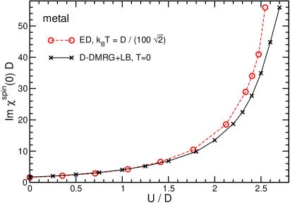
Figure 11: (color online) Static susceptibility $\chi^{\text{spin}}(0)$ from our dynamic data via (19) (black crosses) compared to data obtained by exact diagonalization at very small temperature (red circles), adapted from Fig. 44 in Ref. Georges et al., 1996. The black cross at $U=0$ corresponds to the analytic result $\chi^{\text{spin}}(0)=16/(3\pi D)$. Lines are guides to the eye only.

The curves are dominated by a prominent peak at low frequencies. In some curves, in particular between $U=1D$ and $2D$, there appears to be a shoulder to this peak. Since this feature occurs already for moderate values of $U$ where the curves are still fairly smooth we are confident that this shoulder is in fact a real physical feature. But due to the deconvolution procedure involved we cannot at present rule out completely that it is a spurious numerical effect. In the following we refrain from discussing the shape of the low-frequency peak.

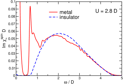
Figure 12: (color online) Positive imaginary part $\chi^{\text{spin}}_{+}$ of the local spin susceptibility as function of frequency for interaction $U=2.8D$ in the metallic and insulating phase.

At higher frequencies around $\omega\approx 2D$ in Fig. 9 a very broad peak of low amplitude can be seen. Qualitatively, this continuum results from the convolution of the lower and the upper Hubbard band or more complicated descriptions in terms of excitations from the lower and the upper Hubbard band.Logan et al. (1998); Galpin and Logan (2008) It corresponds to the continuum found in the insulating phase in Fig. 7.

The insulating and the metallic response at higher frequencies are alike, see Fig. 12, because their single-particle spectral densities are identical for higher frequencies for $U\to U_{c2}$, see Fig. 2 in Ref. Karski et al., 2005. This is analogous to what we have discussed in the charge response in Fig. 4. In both cases, the insulating and the metallic responses coincide for $\omega\gtrapprox 3D$. The slightly more wiggly metallic spin response in Fig. 12 results from the difficulty to deconvolve the relatively small continuum close to the dominating low-frequency peak.

Since the low-frequency peak is clearly the dominating feature its physical significance has to be elucidated. Clearly, it is shifted towards zero frequency on $U\to U_{c2}$ while becoming narrower and narrower. So it is to be expected that it represents the precursor in the metal of the $\delta$ peak in the insulating regime. In order to support this claim we analyze the sum rule (17) and the weight in the low-frequency peak. Both sets of data are depicted for the metal in Fig. 8 by the open symbols. The sum rule is again well fulfilled to within a absolute relative error of $0.5\%$. The weight in the low-frequency peak is integrated till the first minimum in the spectral density on the right hand side of the peak is reached. First, we note that the total spectral weight of the metal equals the one of the insulator for $U\to U_{c2}$ as far as the extrapolation can be trusted. This is expected since the transition occurs precisely where the double occupancies become equal.Karski et al. (2005); Blümer and Kalinowski (2005)

Second, we note that also the weight of the dominant low-frequency peak in the metal approaches the weight of the $\delta$ peak in the insulator to very good accuracy. This clearly corroborates our hypothesis that the metallic dominant low-frequency peak is the precursor of the bound state at zero frequency in the insulator. Naturally, there is no sharp bound state in the metal because such a state can decay into particle-hole states made from the heavy quasiparticles and -holes which are still present in the metal. Hence no bound state but a resonance occurs. The width of this resonance can be understood as Landau damping.

Recall that the low-energy spin resonance in the gapless case becomes the zero-frequency mode of the corresponding gapped case in single impurity Anderson models.Galpin and Logan (2008) So our analysis is well-founded also on the level of the impurity models.

In the insulating regime we have tentatively carried our infinite dimensional results over to finite dimensions. We have speculated that the $\delta$ peak in Fig. 7 becomes a dispersive magnon, if magnetic long-range order exists, or a dispersive triplon if not. Both, magnon or triplon, are bound states of particle-hole pairs from the electronic point of view. So we expect that the emergent magnetic resonance found here becomes in finite dimensions a dispersive resonance which is the precursor of a perfectly sharp magnetic excitation. In literature, the term ‘paramagnon’ is used for such precursive resonances. If no magnetic order is to be expected the term ‘paratriplon’ would be more appropriate.

We recall that the existence of precursive magnetic excitations and their interaction with the single-particle excitations is very important for the understanding of kinks in the electronic dispersionsRaas et al. (2008); Byczuk et al. (2007) and possibly also for Cooper pairing in strongly interacting systems.

IV Conclusions

In this paper, we investigated the zero temperature Mott transition as function of the interaction in a generic model, namely the half-filled Hubbard model in infinite dimensions. We focused on the susceptibilities which are of theoretical and experimental relevance. Thereby, complementary information to the existing investigations of the single-particle dynamics is provided.

We showed that in infinite dimensions the generic susceptibilities are the local ones. Locally, only three types of bosonic observables exist: the charge, the spin and the Cooper pairing operator. So we discussed the corresponding susceptibilites $\chi^{\text{charge}}$, $\chi^{\text{spin}}$, and $\chi^{\text{pair}}$. By an intricate symmetry, $\chi^{\text{pair}}$ is found to be identical to $\chi^{\text{charge}}$.

For the charge susceptibility $\chi^{\text{charge}}$ in the insulating phase we found a strong suppresion on increasing repulsive interaction. The spectral density sets in at $2\Delta$, i.e., at twice the single-particle gap. No binding phenomenon occurs; the spectral line is rather featureless.

In the metallic phase, three ranges in frequency can be distinguished. The first results from a heavy quasiparticle and a heavy quasihole, the second from one heavy excitation and one in one of the two Hubbard bands, and the third consists of a particle in the upper and a hole in the lower Hubbard band. On approaching the insulator $U\to U_{c2}$ the quasiparticle weight $Z$ vanishes linearly.Moeller et al. (1995); Bulla (1999); Karski et al. (2005) The weight in the first region vansihes like $Z^{2}$, the weight in the second region like $Z$ while the weight in the third region, though small, persists. It is also found in the insulator.

A shoulder occurs in the metallic charge response at the same energies as the sharp feature found previously at the inner band edges.Karski et al. (2005, 2008) The weight in the shoulder scales like $Z^{2}$ so that we are led to the conclusion that the shoulder is a consequence rather than the cause of the sharp feature in the single-particle propagator.

The spin susceptibility $\chi^{\text{spin}}$ in the insulating phase is found to be dominated by a strong $\delta$ peak which would correspond in finite dimensions to dispersive magnetic excitations. In infinite dimensions in a paramagnetic insulator it happens to be at zero frequency. The peak must be seen as a particle-hole bound state.

Besides this peak only a very weak continuum is found at higher frequencies. Hence the localized magnetic moment is only very weakly reduced by charge excitations. The Mott insulator is governed by very well localized spins as long as it exists.

In the metallic phase, the spin response at higher frequencies displays again only a continuum of small spectral weight. Upon increasing interaction the spin spectral density is dominated by a pronounced peak at low, but finite, frequencies. This peak comprises most of the spectral weight. It constitutes the precursor of the sharp magnetic mode in the insulator as is evidenced by the coinciding spectral weights of both features at $U=U_{c2}$. The pronounced metallic peak is the signature of an almost bound particle-hole resonance which can be seen as the emergent magnetic mode (paramagnon or paratriplon). We expect this mode to persist in finite dimensions as a dispersive resonance at low, but finite frequencies.

This concludes the investigation of the zero temperature Mott transition at half-filling in infinite dimensions. Further investigations away from half-filling are called for. Similarly, it would be very important to verify the hypotheses derived here for finite dimensions by future calculations.