Modeling phase behavior for quantifying micro-pervaporation experiments

Abstract

We present a theoretical model for the evolution of mixture concentrations in a micro-pervaporation device, similar to those recently presented experimentally. The described device makes use of the pervaporation of water through a thin PDMS membrane to build up a solute concentration profile inside a long microfluidic channel. We simplify the evolution of this profile in binary mixtures to a one-dimensional model which comprises two concentration-dependent coefficients. The model then provides a link between directly accessible experimental observations, such as the widths of dense phases or their growth velocity, and the underlying chemical potentials and phenomenological coefficients. It shall thus be useful for quantifying the thermodynamic and dynamic properties of dilute and dense binary mixtures.

1 Introduction

The thermodynamic and kinetic behavior of dense solutions is of central interest in a number of industrial and scientific activities. The so-called “formulation” of multi-component systems for the production of cosmetics, paints and also comestible goods are industrial examples industry . Scientific interests range from mobilities of macromolecules in cells to the statistical physics and material properties of colloidal suspensions cells ; RusSavSch89 and other mixtures. In all these applications it is important to know the diffusivity or mobility of solutes, their permeability with respect to a solvent or other solutes and similar non-equilibrium quantities. Eventually, dense mixtures are complex substances which are likely to undergo a number of thermodynamic and dynamic transitions of state, which makes their analysis a challenge.

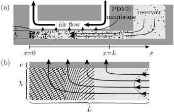
Figure 1: (a) Schematic side view of the micro-evaporator device. It comprises a thin PDMS membrane (thickness $e{\approx}20\mu\textrm{m}$) which allows water to pervaporate out of the lower channel which is filled by a solution ($h{\approx}100\mu\textrm{m}$, $L{\approx}1\textrm{cm}$). (b) More details of the flow pattern: The pervaporating solvent induces also a concentration profile of trapped solute at the end of the channel, here in several dense phases as indicated by the different patterns.

The thermodynamic and dynamic properties of dilute and dense mixtures are usually measured by experimental techniques such as sedimentation/centrifugation, ultra-filtration or reverse osmosis PepEllWor05 ; LebLewSch02 ; Paul04 . Depending on the properties of the solution under investigation, one or the other technique proves to be advantageous. Recently, a promising new microfluidic tool for the analysis of aqueous solutions has been introduced, the microevaporator LenLonTabJoaAjd06 ; LenJoaAjd07 . The employed method is applicable to a wide range of different solutes, such as electrolytes, surfactants, colloids, or polymers. It makes use of the pervaporation of the solvent water through a thin membrane (short vertical arrows in Fig. 1a). The solutes cannot pass the membrane and build up a concentration profile in an underlying microfluidic channel (black dots in Fig. 1a). This profile of solute concentration contains information on the transport coefficients of the mixture. In experiments, the method has been successfully employed for the semi-quantitative screening of equilibrium phase diagrams and the determination of transport coefficients near equilibrium SalLen08 . As a tool for determining phase diagrams, the microevaporator resembles the functionality of the “phase chip” Fraden ; Baitz . However, the microevaporator allows to go one step further towards the controlled analysis of out-of-equilibrium situations.

The quantitative interpretation of the experimental observations in the microevaporator, that is the extraction of the transport coefficients, requires a theoretical model. The observed quantities are spatio-temporal profiles of solute densities, the texture of occurring phases, and the growth dynamics of dense phases which present a moving phase interface. The link between these observables on one side and the underlying thermodynamic equation of state, the transport coefficients of the mixture, and possibly more detailed kinetic parameters on the other side can only be achieved by a sufficiently detailed theoretical model. At the moment, no theoretical model exists for the concentration process caused by pervaporation. We here start to fill this gap.

A model for the phase behavior in microevaporation is subject to the following constraints: On one hand, the microevaporator device can be applied to very different types of solutes, such as colloids, surfactants and electrolytes. Consequently, a sufficiently general theoretical modeling is required which includes phase transitions and out-of-equilibrium phenomena namely metastable phases and precursor phases. It must further take into account the influences of the driving conditions and of the design parameters of the channels. On the other hand, the model should turn the microevaporator into a quantitative tool, making the extraction of thermodynamic and kinetic properties of mixtures possible in a systematic and unambiguous way. This aim requires a sufficiently simple model which permits to approach several limits analytically, and which lends itself to a fast numerical solution of the equations.

The model proposed here can thus be seen as a first compromise between the complexity of the subject, including out-of-equilibrium properties, and the requirement to allow a fast and direct comparison of its solutions with experimental observations.

In order not to overload the description, we restrict it to binary mixtures (water plus a single solute) which are described by two spatio-temporal fields, namely the concentration of solute $\phi(x,t)$ and a velocity $v(x,t)$ of the mixture. The evolution of these two variables is governed by equations of the convection–diffusion type, which comprise two transport coefficients, namely $D(\phi)$ for inter-diffusion of solute and water, and $q(\phi)$ for the pervaporation. Both coefficients are state-dependent, which is indicated by their dependence on the concentration profile $\phi$.

The structure of the paper is the following: In the rest of the current section we give a rough and qualitative description of the physics at work, exemplified for a typical pattern of dense phases such as the one in Fig. 1b. This specific example will be taken up again in the last section of the paper. Section 2 is dedicated to the detailed derivation of the model proposed in this paper. It addresses in two distinct subsections the modeling of the mixture behavior in the microfluidic channel and the pervaporation through the membrane. All steps and assumptions made during the derivation of the final equations are explained in the subsections. After the derivation of the general equations we continue to explore several limit cases. The section ends with a summary of the model equations and the underlying assumptions. In Sec. 3 we focus on situations without phase change, where we will study the smooth concentration profile of solute in the dilute and the dense limits. In the following Sec. 4 we then treat interfaces between different phases occurring in the mixture. The motion of a single moving interface is described first, with the aim to extract its dependence on the properties of the mixture. Then, we return to the introductory example and analyze the thicknesses of several phase slabs. This last analysis is done in a quasi-stationary approximation. Both sections 3 and 4 employ numerically obtained solutions of the model equations and their analytical approximations. We finish with a summary and an outlook in Sec. 5.

1.1 The experimental parameters

The experimental technique and the production of the microevaporator device are detailed in Refs. LenLonTabJoaAjd06 ; LenJoaAjd07 ; SalLen08 . In the theoretical treatment in the present paper, we refer only to the most essential properties of the device. They are displayed in Fig. 1. We use three geometrical parameters, the length $L$ of the PDMS membrane, its thickness $e$ and the height $h$ of the channel containing the solution. The mixture enters the channel from a reservoir with a given solute concentration $\phi_{L}$. This concentration is fixed from outside by the experimenter.

The mixture is driven out of equilibrium by the application of an air flow above the PDMS membrane (thick arrows in Fig. 1a). The air flow guarantees that the pervaporated water is constantly removed from the membrane and that the permeation continues until the solute “dries” out. The out-of-equilibrium situation is thus limited by the slow pervaporation. The experimenter’s second control parameter is the humidity in the air flow. In the case of nearly saturated wet air no pervaporation takes place, because the chemical potentials of water on both sides of the PDMS membrane will become equal. In general, the two external “knobs,” namely the reservoir concentration $\phi_{L}$ and the air humidity need not be constant but can be changed according to a temporal protocol.

Due to the slow pervaporation process, a typical experiment takes hours to days. According to Ref. LenLonTabJoaAjd06 , the intrinsic time scales of the device are in the range of seconds (for the evaporation and the mechanical adjustment of the membrane) up to fifteen minutes (for the diffusion). We may therefore hope that the mixture is not too “far from equilibrium,” which is a necessary requirement for the following description.

During the evaporation, several quantities can be measured, such as the total amount of mixture which passes through the device during the experiment. It gives some information on the amount of solute in the channel and on the rate of water pervaporation. Within the channel, more information on the mixture can be gathered: If there are several phases in the mixture and if they can be differentiated e.g. by their texture, then the position of the interfaces can be tracked as a function of time. This has been done for the case of the surfactant AOT (docusate sodium salt) in water in Ref. LenJoaAjd07 and for a salt solution in Ref. LenLonTabJoaAjd06 . More information is obtained if the full density profile can be measured as a function of time LenLonTabJoaAjd06 . These types of observables are in the focus of the present theoretical description.

1.2 An intuitive example

The central interest of the present theoretical description is the precise functional forms of two coefficients, one of which is the inter-diffusion coefficient $D(\phi)$ of solute and solvent, the other one $q(\phi)$ quantifies the pervaporation of solvent through the PDMS membrane. Both coefficients do depend on the local concentration $\phi(x,t)$ of solute. All thermodynamic and kinetic properties of the mixture are implicitly contained in these two coefficients. In particular, they can be expressed in terms of the chemical potentials and of the kinetic properties of the mixture, both of which depend on $\phi$.

Suppose the situation in Fig. 1b, which has been explored experimentally using the surfactant AOT (docusate sodium salt) in water LenJoaAjd07 : The channel is filled by four different phases of the mixture, which are ordered by their solute concentration. Three of them are dense, indicated by different patterns in Fig. 1b, the fourth phase is dilute. The pervaporation of water, quantified by introducing the coefficient $q(\phi)$ gives rise to a flow from the reservoir (long curved arrows) which compensates the water loss at the PDMS membrane. On its way through the phases the water drags the solute with it. It thereby induces the concentration of solute, and, at higher and higher concentration, the appearance of the three dense phases which would be absent without flow.

The final concentration profile is thus a dynamic equilibrium between convective and diffusive processes: Within each phase slab the concentration gradient gives rise to diffusion which in turn tries to shrink the phases. While the diffusion emerges together with the concentration gradients, the convective transport, or “drag” is reduced by the solute becoming dense. The solvent has to permeate through the dense phases of solute before it reaches the membrane and pervaporates. The denser the solute, the less solvent may pass. Furthermore, the more the water flow tries to compress, or to “squeeze” the dense phases, the harder it becomes to squeeze them even further. One or the other of the mentioned mechanisms may remind the reader of terms such as “osmotic compressibility,” “diffusion,” “mobility,” “permeability,” depending on the liking and the experience of the reader. In fact, all these effects are linked to one another, and we will provide the connection between some of these terms in Sec. 2.3. We thereby also show the equivalence of these terms, in so far as they can expressed one by the other. In our model we abandon the use of terms such as mobility, osmotic compressibility and permeation in favor of the diffusion coefficient $D(\phi)$ and the coefficient of pervaporation $q(\phi)$, which are expressed in terms of the chemical potential of water and of the phenomenological coefficient for inter-diffusion.

An important observation in the situation of Fig. 1b is the following: As more and more solute is transported from the reservoir, all three dense phases grow. It has been observed experimentally that the two interior “sandwiched” phases apparently grow at constant thickness. They loose as much solute as they gain, while the last, the most dense phase continues to grow. Keeping in mind the dynamic equilibrium between convective and diffusive processes within each phase we therefore find in the thicknesses of these middle phases a fingerprint of the diffusion coefficient and of the pervaporation coefficient.

One may now ask whether a large diffusion coefficient will finally lead to a thinner or to a thicker slab, as compared to one with a smaller diffusion coefficient? On one hand, the diffusion coefficient scales the gradients of the concentration profile which try to dissolve the phases. It should thus lead to small thicknesses of the quenched dense phases. On the other hand, for fixed values of the concentration at the phase interfaces, a large diffusion coefficient will render the profiles flat and therefore lead to thick phases. This may appear paradoxical on a first sight, but it only reflects the same feedback mechanism as between flow of solvent and permeability. The resolution is that we really need the full concentration profile and the velocity field in order to understand the phase thicknesses.

2 Detailed derivation of the model

In this section we derive a set of equations which model the evolution of a binary system, reduced to one spatial dimension $x$ along the evaporation channel. As variables of state we use a concentration $\phi(x,t)$ of solute and a mixture velocity $v^{0}(x,t)$. Special focus will be put on their precise meaning in the evolution equation that will be derived in the following sections,

$$\partial_{x}v^{0}=-\nu_{w}q(\phi),$$ (1)

$$\partial_{t}\phi=-\partial_{x}\bigl{[}\phi v^{0}-D(\phi)\partial_{x}\phi\bigr{]}.$$ (2)

Here, $\nu_{w}$ denotes the specific mass of water; $\partial_{t}$ and $\partial_{x}$ are partial derivatives with respect to time and space. The physical content of the equations is the independent balance of solvent and solute mass. The variables are chosen such that $q(\phi)$ reflects the loss of solvent (water) via pervaporation, and $D(\phi)$ is a state-dependent inter-diffusion coefficient, which contains information on the thermodynamic and dynamic properties of the mixture. The expressions for $D(\phi)$ and $q(\phi)$ will be provided by equations (31) and (46) below.

2.1 Diffusion model for the binary solution

The aim here is to state clearly all underlying assumptions which lead to the model equations (1) and (2), starting from mass conservation. This procedure will allow to point out the restrictions of the model. We employ the theory of linear out-of-equilibrium thermodynamics as summarized in the book by de Groot and Mazur GroMaz84 . We try to adopt the notation used there, also for an easier comparison with the results by Peppin et al. PepEllWor05 for the link to sedimentation, ultra-filtration, and reverse osmosis.

2.1.1 Balance equations for binary mixtures

The balance equations for the mass densities $\rho_{s}(\mathbf{r},t)$ and $\rho_{w}(\mathbf{r},t)$ of solute (index $s$) and solvent (index $w$) read

$$\partial_{t}\rho_{k}=-\operatorname{div}(\mathbf{j}_{k}),\quad\text{with $k\in\{s,w\}$.}$$ (3)

The mass current densities $\mathbf{j}_{k}$ are split into an advected and a diffusive part,

$$\mathbf{j}_{s}=\rho_{s}\mathbf{v}_{s}=\rho_{s}\mathbf{v}+\mathbf{J}_{s},$$ (4)

$$\mathbf{j}_{w}=\rho_{w}\mathbf{v}_{w}=\rho_{w}\mathbf{v}+\mathbf{J}_{w}.$$ (5)

The $\mathbf{J}_{i}$ denote the “diffusive currents”, simply defined by the difference $\rho_{i}(\mathbf{v}_{i}-\mathbf{v})$. A common choice for the mixture velocity is the mass-average of the individual constituent velocities $\mathbf{v}_{k}$, weighted by the mass fractions $c_{k}$,

$$\mathbf{v}:=\sum_{i}c_{i}\mathbf{v}_{i}$$ (6)

$$\text{with}\quad c_{i}:=\frac{\rho_{i}}{\rho}\quad\text{and}\quad\rho:=\sum_{k}\rho_{k}.$$ (7)

This choice makes the two diffusive currents opposite to each other,

$$\mathbf{J}_{w}=-\mathbf{J}_{s}.$$ (8)

Formally, the mass densities are taken to be functions of the local thermodynamic variables of state as $\rho_{i}(T,P,c_{s})$. The use of local temperature and pressure fields shows that here and in the following we will assume local thermodynamic equilibrium. The evolution equations (3) are accompanied by the following constraint, which is an immediate consequence of the chemical potentials being intensive quantities (or of the Euler relation),

$$1=\nu_{s}\rho_{s}+\nu_{w}\rho_{w}.$$ (9)

The specific volumes per mass, $\nu_{i}$, are defined as the derivatives of the chemical potentials per mass, $\gamma_{i}(T,P,c_{s})$, with respect to the pressure,

$$\nu_{i}(T,P,c_{s}):=\left.\frac{\partial\gamma_{i}}{\partial P}\right|_{T,c_{s}}.$$ (10)

$$\gamma_{i}(T,P,c_{s}):=\frac{\mu_{i}(T,P,c_{s})}{m_{i}}.$$ (11)

Here, $\mu_{i}$ is the chemical potential per molecule, and $m_{i}$ the mass of such a molecule. The derivative in Eq. (10) equals the change of volume induced by adding an infinitesimal amount of mass of type $i$ upon keeping temperature, pressure and all remaining masses constant. Equation (9) can be used to introduce the volume fractions $\phi_{i}(T,P,c_{s}):=\nu_{i}\rho_{i}$. Below, equation (9) will also be the point of entrance for the notion of simple mixtures and of incompressibility of the constituents. Apart from Eq. (9), another consequence of the intensivity of chemical potentials is the following relation between the derivatives of the two chemical potentials with respect to the mass fraction of solvent, $c_{s}$,

$$c_{s}\frac{\partial\gamma_{s}}{\partial c_{s}}\biggr{|}_{T,P}=-(1-c_{s})\frac{\partial\gamma_{w}}{\partial c_{s}}\biggr{|}_{T,P}.$$ (12)

This equation establishes the standard logarithmic behavior of the chemical potentials in the limits $c_{s}\to 0$ and $c_{s}\to 1$.

Together, equations (9) and (12) reduce the number of relevant chemical potentials to one, as one can always be expressed by the other. This fact is important for the number of kinetic coefficients within the theory of linear non-equilibrium thermodynamics. Applying this framework in the present description, the diffusive current $\mathbf{J}_{s}$ is taken to be proportional to the gradients of chemical potentials. The proportionality factor is called the phenomenological coefficient $\mathcal{L}$. Using the relation of Gibbs-Duhem, only the difference of chemical potentials can occur, and we receive for the diffusive current

$$\mathbf{J}_{s}=-\mathcal{L}\>\boldsymbol{\nabla}(\gamma_{s}-\gamma_{w}).$$ (13)

We do not present the details of the derivation of this equation here, as it implies a rather tedious consideration of all possible symmetries in the entropy production. Instead, we refer to Eq. (IV.15) in the book by de Groot and Mazur GroMaz84 or to the summary in the paper by Peppin et al. PepEllWor05 . Note that external forces such as gravity cancel out and do not appear in equation (13). This fact is due to the chemical potentials being defined as energy per mass rather than per number of particles. Furthermore, we have omitted a term proportional to the temperature gradient, as from now on we take the temperature as uniform and constant. We will omit it also from the argument lists of thermodynamic functions. The phenomenological coefficient $\mathcal{L}$ may in principle depend on all thermodynamic variables of state as well as on their derivatives, and even on the mixture velocity $\mathbf{v}$ and its derivatives. However, if the assumption of local thermodynamic equilibrium is well satisfied, the dependence on the mixture velocity field should be negligible, such that we use a function $\mathcal{L}(P,c_{s})$ for the moment. The chemical potentials are also functions of the two thermodynamic parameters: $\gamma_{s}(P,c_{s})$ and $\gamma_{w}(P,c_{s})$. This functional dependence allows to separate the influence of pressure gradients from concentration gradients in Eq. (13),

$$\mathbf{J}_{s}=-\mathcal{L}\>\Bigl{[}(\nu_{s}-\nu_{w})\boldsymbol{\nabla}P+\frac{\partial(\gamma_{s}-\gamma_{w})}{\partial c_{s}}\Bigr{|}_{T,P}\boldsymbol{\nabla}c_{s}\Bigr{]}.$$ (14)

With the aid of relation (12) the diffusive second term can be rephrased using either of the chemical potentials,

$$\frac{\partial(\gamma_{s}-\gamma_{w})}{\partial c_{s}}\Bigr{|}_{T,P}=\frac{1}{1-c_{s}}\frac{\partial\gamma_{s}}{\partial c_{s}}\Bigr{|}_{T,P}=-\frac{1}{c_{s}}\frac{\partial\gamma_{w}}{\partial c_{s}}\Bigr{|}_{T,P}.$$ (15)

Equation (14) has been used by Peppin et al. (PepEllWor05, , Eq. (28)) to demonstrate that Fick’s and Darcy’s laws are limiting cases of the same equation. Below, we will use it to define the diffusion coefficient and to make the connection between the different methods micro-pervaporation, sedimentation, and ultra-filtration.

2.1.2 Reduction to 1D

We shall now disregard the details of the flow pattern in the channel and reduce the three-dimensional evolution equations (3) to one dimension. We do this by averaging over the two spatial dimensions perpendicular to the channel axis, as depicted in Fig. 2. For a given uniform height $h$ and width $b$ of the channel we obtain from integration over a slice $\Omega$ with area $|\Omega|=bh$ the one-dimensional counterparts of (3),

$$\partial_{t}\rho_{s} =-\partial_{x}j_{s}$$ (16)

$$\partial_{t}\rho_{w} =-\partial_{x}j_{w}-q.$$ (17)

The new densities and currents turn out to be

$$\rho_{k}(x,t):=\frac{1}{|\Omega|}\int_{\Omega}dy\,dz\>\rho_{k}(x,y,z,t),$$ (18)

$$j_{k}(x,t):=\frac{1}{|\Omega|}\int_{\Omega}dy\,dz\>\mathbf{e}_{x}\boldsymbol{\cdot}\mathbf{j}_{k}(x,y,z,t).$$ (19)

The water loss due to pervaporation through the PDMS membrane is all included in $q(x,t)$. It represents the integral of water current in normal direction over the boundary of the channel,

$$q(x,t) :=\frac{1}{|\Omega|}\int_{\partial\Omega}\mathbf{N}\boldsymbol{\cdot}\mathbf{j}_{w}(x,y,z,t)$$ (20)

$$\approx\frac{1}{b\,h}\int_{0}^{b}\mathbf{N}\boldsymbol{\cdot}\mathbf{j}_{w}(x,y,h,t)\,dy.$$ (21)

The pervaporation has a dominant contribution from the upper boundary where the thin layer of PDMS allows a steady water pervaporation. In addition to equations (16) and (17) we expect an averaged version of constraint (9) to hold. In the same manner as above in Eqs. (4) and (5) we may subdivide the total currents into advective and diffusive parts.

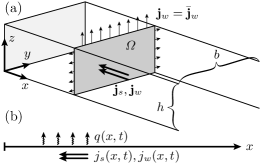
Figure 2: Visualization of the averaging used for reducing the balance equations to one dimension. (a) The area of integration $\Omega$ in three dimensions. (b) The one-dimensional representation.

2.1.3 Incompressibility and simplicity of mixtures

We now assume both constituents of the mixture to be individually incompressible, having constant specific volumes $\nu_{i}$. This assumption will allow to reduce the set of three equations (16), (17), and (9) to only two equations. The assumption, however, is quite strong as it implies the mixture to be both incompressible and simple,

$$\frac{\partial 1/\rho}{\partial P}\biggr{|}_{T,c_{s}}=0,\qquad\frac{\partial 1/\rho}{\partial c_{s}}\biggr{|}_{T,P}=\nu_{s}-\nu_{w}=\textit{const.}$$ (22)

The term simple mixture here means that the total mass density is a linear function of the mass fraction. It implies linear relations between mass density, mass fraction and volume fraction. We will therefore use the terms “density”, “fraction” and “concentration” interchangeably. Simple mixtures are for example glycerol in water JosHuaHu96 or rigid spheres in an incompressible solvent of much smaller particles. The constraint (9) allows to write one density as a function of the other, $\rho_{w}=\rho_{w}(\rho_{s})$. The evolution equation (17) for $\rho_{w}(\rho_{s})$ then becomes

$$\Bigl{(}\rho_{w}(\rho_{s})-\frac{\partial\rho_{w}}{\partial\rho_{s}}\rho_{s}\Bigr{)}\partial_{x}v+\partial_{x}J_{w}-\frac{\partial\rho_{w}}{\partial\rho_{s}}\partial_{x}J_{s}=-q.$$ (23)

This equation can be understood as a differential equation for the velocity field, similar to the one we are looking for (1). However, the occurrence of the diffusive currents $J_{s}$ and $J_{w}$ makes it unfavorably dependent on the concentration variable, see equations (14) and (8). A more convenient equation is obtained by using from the beginning the volume-averaged mixture velocity

$$v^{0}:=\sum_{i}\phi_{i}v_{i}$$ (24)

instead of the mass-averaged one. The total currents are then written with modified diffusive currents,

$$j_{k}=\rho_{k}v^{0}+J^{0}_{k},\quad k\in\{s,w\}.$$ (25)

With the volume-averaged mixture velocity, and by setting the specific volumes constant, one obtains as relation between the new diffusive currents,

$$J^{0}_{w}=-\frac{\nu_{s}}{\nu_{w}}J^{0}_{s}$$ (26)

instead of equation (8). This property makes the diffusive currents vanish from the differential equation for $v^{0}(x,t)$, which now comes close to the form we seek (1),

$$\partial_{x}v^{0}=-\nu_{w}q(P,\phi).$$ (27)

In terms of the volume-averaged mixture velocity, and with constant $\nu_{s}$, the volume fraction of solute evolves as

$$\partial_{t}\phi_{s}=-\partial_{x}\Bigl{[}\phi_{s}v^{0}+\bigl{(}\nu_{w}\phi_{s}+\nu_{s}(1{-}\phi_{s})\bigr{)}\,J_{s}\Bigr{]}.$$ (28)

Or, omitting the index $s$ and collecting also equations (14) and (15), we finally arrive at

$$\partial_{t}\phi=-\partial_{x}\Bigl{[}\phi v^{0}-K(P,\phi)\partial_{x}P-D(P,\phi)\partial_{x}\phi\Bigr{]},$$ (29)

with the shortcuts

$$K(P,\phi)=[\nu_{s}+\phi(\nu_{w}-\nu_{s})]\>\mathcal{L}(P,\phi)\>(\nu_{s}-\nu_{w}),$$ (30)

$$D(P,\phi)=-\frac{[\nu_{s}+\phi(\nu_{w}-\nu_{s})]^{2}}{\nu_{w}\phi}\>\mathcal{L}(P,\phi)\>\frac{\partial\gamma_{w}}{\partial\phi}\Bigr{|}_{T,P}.$$ (31)

Equations (27) and (29) with the coefficients $q$ and $D$ from (20) and (31) come close to the model we announced in the introduction. They nicely separate the effect of pervaporation, which is all contained in the coefficient $q$, from the bulk thermodynamic and kinetic properties of the mixture. These properties are implicitly contained in the functional dependence of $\mathcal{L}$ and $\gamma_{w}$ on $P$ and on $\phi$.

2.1.4 The role of the pressure gradient

With equations (27) and (29) we have found two equations for yet three variables $v^{0}$, $\phi$, and $P$. We thus have to seek for a closure of the above set of equations. The contribution by the pressure requires some further attention. The pressure occurs as an argument in several functions, but also its gradient adds a contribution to the diffusive current in Eq. (29). This gradient appears also in the (compressible) Stokes equation. In principle, it would have been possible to assume local mechanical equilibrium already in the 3D theory, such as the $x$-component of the compressible Stokes equation,

$$0=-\partial_{x}P+\eta\Delta v_{x}+(\lambda+\eta/3)\partial_{x}\operatorname{div}\mathbf{v}$$ (32)

and then reduce it to one dimension together with fitting boundary conditions. The shear and bulk viscosities are denoted by $\eta$ and $\lambda$, respectively. However, this procedure raises fundamental difficulties: We showed above that the natural description of pervaporation of incompressible mixtures involves the volume-averaged velocity $v^{0}$. The natural formulation of the Stokes equation uses the mass-averaged velocity. Only for the special case $\nu_{s}=\nu_{w}$ both velocities do coincide—but in this very case the term with $\partial_{x}P$ vanishes due to $K=0$. When expressing $\mathbf{v}$ by $\mathbf{v}^{0}$, the term with $\partial_{x}P$ in Eq. (29) will contribute to both other terms in the expression for the diffusive current in (29). We do even expect a coupling of velocity and density variables, as well as a second derivative $\partial_{x}^{2}\phi$ due to the second derivatives in the Stokes equation (32).

The precise analysis of this splitting is beyond the scope of the present paper. Here, we have to restrict the validity of the model to cases where the influence of the pressure gradient is negligible. An estimation footnote3 indicates that this restriction is indeed weak: In the dilute limit, using values from the experiment LenLonTabJoaAjd06 , the term with the pressure gradient in Eq. (29) is several magnitudes smaller than the diffusion term with the concentration gradient. In what follows we therefore use the simplistic model with a homogeneous pressure variable (which we omit in the notation from now on):

$$\partial_{x}v^{0}=-\nu_{w}q(\phi),$$ (33)

$$\partial_{t}\phi=-\partial_{x}\Bigl{[}\phi v^{0}-D(\phi)\partial_{x}\phi\Bigr{]}.$$ (34)

with the evaporation coefficient $q(\phi)$ and the diffusion coefficient $D(\phi)$, both depending only on the volume fraction $\phi$.

As we take the microevaporation channels to be horizontal, our assumption of setting the pressure gradient to zero coincides with the assumptions employed by Peppin et al. PepEllWor05 and also in the context of sedimentation RusSavSch89 where the pressure gradient balances gravitational forces. It therefore opens the possibility to consistently compare with their model equations, see Sec. 2.3.

2.1.5 Boundary conditions

Equations (33) and (34) are to be accompanied by an appropriate number of boundary conditions. For the hyperbolic differential equation (33) we require one, for the parabolic equation (34) we need two boundary conditions. At the end of the channel, both the mixture velocity and the total solute current vanish,

$$v^{0}(0,t)=0,$$ (35)

$$\partial_{x}\phi(0,t)=0.$$ (36)

As a third boundary condition we use a fixed concentration at the inlet of the channel, reflecting the concentration in the reservoir,

$$\phi(L,t)=\phi_{L}.$$ (37)

The model equations could equally handle a time-dependent reservoir concentration $\phi_{L}(t)$. In a setup with a fixed total amount of solute in the channel, it is mathematically also possible to replace the latter boundary condition by an integral condition setting $\int_{0}^{L}\phi(x,t)\,dx$ to a given value.

2.1.6 Moving interfaces between phases

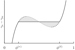
Figure 3: Sketch of the modeling of sharp interfaces between different phases. The concentration values left and right of the interface are fixed by a Maxwell construction on the chemical potential (upper panel), the two regions shaded in gray have equal area.

In the introductory example we mentioned that the positions of phase interfaces and their velocities are convenient observables in the pervaporation experiments. Such experimental observations have been reported in Ref. LenLonTabJoaAjd06 and in more detail in Ref. LenJoaAjd07 for a solution of the surfactant AOT (docusate sodium salt) in water. The essential observation in the latter reference is the decrease of the interface velocity with time, which will be investigated in more detail below in section 4.1. A quantitative analysis of this decrease can give insight into the mechanisms at work, especially on the relative importance of diffusion and advection caused by pervaporation.

Throughout this paper, we model the interfaces within the framework of local equilibrium thermodynamics, which implies that the interfaces are infinitely sharp and that for each such interface there are two unique concentration values at its left-hand and its right-hand sides. These values are determined by a Maxwell construction on the local chemical potential function. Figure 3 sketches this construction and the resulting concentration profile around the interface. The fixed concentration variables serve as two Dirichlet boundary conditions for the evolution equation (34),

$$\phi\bigl{(}X^{(\ell)},t\bigr{)}=\phi^{(\ell)},\quad\phi\bigl{(}X^{(r)},t\bigr{)}=\phi^{(r)}.$$ (38)

The superscripts ${(\ell)}$ and ${(r)}$ indicate the left and right limits towards the interface position $X(t)$.

The conservation of solute mass, which is valid also across the interface, provides us with a continuity condition at the interface. If the boundary does not move, the solute currents at the left-hand and at the right-hand sides of the interface must coincide. Any possible difference between these incoming and outgoing currents must lead to a growth of one phase and thus to the movement of the interface position $X(t)$. Its velocity times the concentration jump at the surface must equal the difference between the currents,

$$\dot{X}(t)=\frac{j_{s}\bigl{(}X^{(\ell)},t\bigr{)}-j_{s}\bigl{(}X^{(r)},t\bigr{)}}{\phi^{(\ell)}-\phi^{(r)}}.$$ (39)

We further require continuity conditions for the velocity field. As we did in the derivation of the bulk equations, we also here want the mixture velocity to reflect only the influence of the pervaporation. As we do not expect the pervaporation to diverge near phase interfaces, the velocity field should be continuous across such an interface,

$$v^{0}(X^{(\ell)},t)=v^{0}(X^{(r)},t).$$ (40)

This continuity equation is consistent with the conservation of solvent mass across the interface.

2.2 Pervaporation through the PDMS membrane

The pervaporation of water through the PDMS layer can be described on the same level as the advective and diffusive currents in the evaporation channel. We now focus on the binary mixture of water and PDMS, as solutes cannot enter the PDMS domain. The notation is such that the properties inside the PDMS membrane will be denoted by an overbar. As we did above, we also here split the total current density $\bar{\mathbf{j}}_{w}$ of water into convective and diffusive terms. This time it is more convenient to take the velocity of PDMS, which is zero, as the reference velocity of the mixture. The mass current density of water in the layer then becomes

$$\bar{\mathbf{j}}_{w}=\frac{1}{1-\bar{c}_{w}}\bar{\mathbf{J}}_{w},$$ (41)

where $\bar{c}_{w}$ is the mass fraction of water inside the layer, and $\bar{\mathbf{J}}_{w}$ is the corresponding diffusive current. In complete analogy to equation (13), the diffusive current can be written in terms of a phenomenological coefficient $\bar{\mathcal{L}}$,

$$\bar{\mathbf{j}}_{w}=-\frac{\bar{\mathcal{L}}(P,\bar{c}_{w})}{1-\bar{c}_{w}}\boldsymbol{\nabla}(\bar{\gamma}_{w}-\bar{\gamma}_{\text{PD}}).$$ (42)

with the chemical potential of PDMS denoted by $\bar{\gamma}_{\text{PD}}$. We understand the pervaporation as a diffusive process and again omit the pressure-dependence of the chemical potentials. Then, the water current is proportional to the gradient of water concentration. The diffusion process is further assumed to be sufficiently established that the water current does not vary within the membrane. In the dilute limit, where the chemical potential exhibits a logarithmic behavior,

$$\bar{\gamma}_{w}(T,P,\bar{c}_{w})=\bar{\gamma}_{w}^{\ast}(T,P)+\frac{kT}{m_{w}}\,\ln\bar{c}_{w},$$ (43)

the uniform water current then corresponds to a constant gradient of water concentration inside the membrane. The water current through the membrane is then proportional to the concentration difference across the membrane of thickness $e$,

$$\mathbf{N}\boldsymbol{\cdot}\bar{\mathbf{j}}_{w}=\frac{\bar{c}_{w}(z{=}h{+}e)-\bar{c}_{w}(z{=}h)}{e}\lim_{\bar{c}_{w}\to 0}\frac{\bar{\mathcal{L}}(P,\bar{c}_{w})}{(1-\bar{c}_{w})^{2}}\frac{\partial\bar{\gamma}_{w}}{\partial\bar{c}_{w}}.$$ (44)

To make the connection with the conditions in the adjacent channels of the mixture and of the air flow, we assume that the chemical potentials at both sides of both boundaries of the PDMS membrane have matching values,

$$\bar{\gamma}_{w}(z{=}h)=\gamma_{w}\quad\text{and}\quad\bar{\gamma}_{w}(z{=}h{+}e)=\gamma_{w}^{\text{air}}.$$ (45)

The evaporation coefficient $q$ can now be expressed as a function of the chemical potential $\gamma_{w}(\phi)$ in the mixture channel. From equations (44), (43), and its definition (21) we finally obtain the following dependence of the pervaporation coefficient on the volume fraction,

$$q(\phi)=\frac{1}{\nu_{w}}\frac{\bar{D}}{eh}\biggl{[}\exp\Bigl{\{}\frac{m_{w}}{kT}\gamma_{w}(\phi)\Bigr{\}}-\exp\Bigl{\{}\frac{m_{w}}{kT}\gamma_{w}^{\text{air}}\Bigr{\}}\biggr{]}.$$ (46)

We have collected several of the above constants in the shortcut $\bar{D}$,

$$\bar{D}=\nu_{w}\exp\Bigl{\{}-\frac{m_{w}}{kT}\bar{\gamma}_{w}^{\ast}\Bigr{\}}\lim_{\bar{c}_{w}\to 0}\bar{\mathcal{L}}\,\frac{\partial\bar{\gamma}_{w}}{\partial\bar{c}_{w}}.$$ (47)

Expression  (46) contains the further assumption that the chemical potential directly at the interface between mixture channel and PDMS layer is the same as the average chemical potential in the mixture which we obtained from the reduction to one spatial dimension. In the present framework of a one-dimensional description, there is no alternative to this approximation.

At the present point we have completed the derivation of the model, consisting of the two differential equations (33) and (34) for the volume fraction $\phi$ and the volume-averaged velocity field $v^{0}$, together with the concentration-dependent diffusion coefficient (31) and the evaporation coefficient (46).

2.3 Connection with sedimentation and ultra-filtration

We now make the connection between the two coefficients $D(\phi)$ and $q(\phi)$ and other pairs of coefficients. This will allow to compare different techniques of measuring chemical potentials and phenomenological coefficients and to verify the consistency of the outcomes. We will not make use of these connections in the present paper. The equations in this section can rather be seen as a convenient reference for the reader working on different techniques. However, the comparisons give some more intuition on the variables and coefficients which are used. Above, in equations (31) and (46) we have already found the link to the pair $\gamma(\phi)$ and $\mathcal{L}(\phi)$. We continue by expressing also the coefficients of sedimentation and of permeability in terms of $\gamma(\phi)$ and $\mathcal{L}(\phi)$. Each of these two coefficients forms together with the diffusion coefficient a pair which allows to determine $\gamma(\phi)$ and $\mathcal{L}(\phi)$ and thus to make the link to our original coefficients $D(\phi)$ and $q(\phi)$.

2.3.1 Sedimentation factor and osmotic compressibility factor

In the context of sedimentation of colloids, Russel, Saville, and Schowalter RusSavSch89 express the thermodynamic and dynamic properties in terms of the sedimentation factor $K^{\text{RSS}}(\phi)$ and the osmotic compressibility factor $Z^{\text{RSS}}(\phi)$. Both can be introduced by rewriting Eq. (29) as follows (RusSavSch89, , compare Eq. 12.5.6),

$$\partial_{t}\phi=-\operatorname{div}\Bigl{(}\phi\mathbf{v}^{0}+\mathbf{U}_{0}\phi K^{\text{RSS}}(\phi)-D(\phi)\boldsymbol{\nabla}\phi\Bigr{)}$$ (48)

with the diffusion coefficient

$$D(\phi)=D_{0}K^{\text{RSS}}(\phi)\frac{d}{d\phi}\bigl{[}\phi Z^{\text{RSS}}(\phi)\bigr{]}$$ (49)

and with the shortcuts

$$D_{0}:=\frac{kT}{6\pi\eta\,a},\quad\mathbf{U}_{0}:=-\frac{2a^{2}}{9\eta}\Bigl{(}\frac{1}{\nu_{w}}-\frac{1}{\nu_{s}}\Bigr{)}\mathbf{g}$$ (50)

with $\eta$ denoting the viscosity of pure solvent, $a$ the radius of a colloidal sphere, and $\mathbf{g}$ the acceleration by gravity. The volume-averaged velocity in Eq. (48) vanishes by construction of the sedimentation experiment in a closed container. In the comparison with Eq. (29) the remaining two terms thus lead us to the sedimentation coefficient $K^{\text{RSS}}$ given as

$$K^{\text{RSS}}(\phi)=\frac{|\boldsymbol{\nabla}P|}{\rho g}\frac{9\eta}{2a^{2}}\nu_{s}^{2}\Bigl{(}1+\phi\frac{\nu_{w}{-}\nu_{s}}{\nu_{s}}\Bigr{)}^{2}\frac{\mathcal{L}(\phi)}{\phi}.$$ (51)

The osmotic compressibility factor, originally defined by the osmotic pressure of solute $\Pi(\phi)$ can equivalently be expressed in terms of the chemical potential of water,

$$Z^{\text{RSS}}(\phi)=\frac{3}{4\pi\,a^{3}}\frac{\Pi(\phi)}{\phi kT}=\frac{3}{4\pi\,a^{3}}\frac{\gamma_{w}(0)-\gamma_{w}(\phi)}{\nu_{w}\phi kT}.$$ (52)

Peppin, Elliott, and Worster PepEllWor05 define the sedimentation coefficient $S^{\text{PEW}}$ in a marginally different way. Their definition leads to the following variant of the transport equation (48) (see Eq. (32) of Ref. PepEllWor05 ),

$$\partial_{t}\phi=-\operatorname{div}\Bigl{(}\phi\mathbf{v}^{0}+\mathbf{g}\phi K^{\text{PEW}}(\phi)-D(\phi)\boldsymbol{\nabla}\phi\Bigr{)}$$ (53)

In their treatment, the pressure gradient is assumed to balance the force density by gravitation, $\boldsymbol{\nabla}P=\rho\mathbf{g}$. In our notation of Eq. (30), their sedimentation coefficient reads

$$S^{\text{PEW}}(\phi)=\frac{K(\phi)}{\phi\nu_{w}}\Bigl{(}1+\phi\frac{\nu_{w}-\nu_{s}}{\nu_{s}}\Bigr{)}.$$ (54)

2.3.2 Permeability

For the coefficient of permeability $k^{\text{PEW}}$ Peppin et al. give the result (Eq. (37) of Ref. PepEllWor05 )

$$\frac{k^{\text{PEW}}}{\eta}=\frac{\mathcal{L}(\phi)\nu_{s}}{\phi^{2}\nu_{w}^{2}}\Bigl{(}1+\phi\frac{\nu_{w}-\nu_{s}}{\nu_{s}}\Bigr{)}^{2}.$$ (55)

Except for the dilute limit, the phenomenological coefficient $\mathcal{L}(\phi)$ can be understood as a direct measure of the permeability of the solute with respect to the solvent. This will be useful below when choosing a model function for $\mathcal{L}(\phi)$. In particular, Eq. (55) helps choosing the value of $\mathcal{L}(1)$, which has influence on the qualitative behavior of the solutions, see the discussion of Fig. 8. In the opposite limit, Eq. (51) indicates that $\mathcal{L}(\phi)\propto\phi$ for small $\phi$. This last requirement leads to a finite non-zero diffusion coefficient in the dilute limit, see below in Fig. 14.

2.4 Summary of the model equations, and their preparation for a numerical implementation

We here summarize the model equations (1), (2), (31), and (46) for their further use in the following sections. We repeat their boundary conditions and the condition for the interface movement. We also reformulate the model equations in such a way that they may be discretized and implemented more easily. The dimensionless equations of evolution (1) and (2) read

$$\partial_{x^{\prime}}v^{0\prime}=-q^{\prime}(\phi),$$ (56)

$$\partial_{t^{\prime}}\phi=-\partial_{x^{\prime}}j^{\prime}=-\partial_{x^{\prime}}\Bigl{[}v^{0\prime}\phi-\frac{D^{\prime}(\phi)}{\mbox{{Pe}}}\partial_{x^{\prime}}\phi\Bigr{]}.$$ (57)

They describe the evolution of an incompressible binary mixture in one effective spatial dimension under the further assumption of homogeneous temperature and pressure. The variables carrying a prime are made dimensionless by the following scales for length ($x$), time ($t$) and the mixture velocity ($v^{0}$). The volume fraction $\phi$ needs no further rescaling. The scales have been chosen such that all dimensionless variables are of the order unity as far as possible,

$$x=Lx^{\prime},\quad t=t^{\prime}/\bigl{(}\nu_{w}q(0)\bigr{)},\quad v^{0}=L\nu_{w}q(0)\,v^{0\prime},$$ (58)

$$q(\phi)=q(0)\,q^{\prime}(\phi),\quad D(\phi)=D(0)\,D^{\prime}(\phi),$$ (59)

$$\mbox{{Pe}}=\frac{L^{2}\nu_{w}q(0)}{D(0)}.$$ (60)

Here, the Peclet number Pe is a global Peclet number of the system. The scales for the diffusion coefficient and the coefficient of evaporation, which are simply the coefficients evaluated at zero concentration density ($D(0)$ and $q(0)$) are chosen such that Pe presents an upper bound for the true (local) Peclet number $\mbox{{Pe}}_{\textit{loc}}(x,t)$ which can only be determined a posteriori from the solution. In numerical solutions we have found the local Peclet number to be always maximal at the entrance of the channel and unity at the end. However, it does not need to be monotonous.

The dimensionless version $q^{\prime}(\phi)$ of the pervaporation coefficient is, according to the expression we found in (46),

$$q^{\prime}(\phi)=\frac{\exp\Bigl{\{}\frac{m_{w}}{kT}\bigl{(}\gamma_{w}(\phi)-\gamma_{w}^{\text{air}}\bigr{)}\Bigr{\}}-1}{\exp\Bigl{\{}\frac{m_{w}}{kT}\bigl{(}\gamma_{w}(0)-\gamma_{w}^{\text{air}}\bigr{)}\Bigr{\}}-1}.$$ (61)

It depends on the volume fraction $\phi$ only via the chemical potential of water $\gamma_{w}(\phi)$, all other parameters are constants or external driving parameters. The dimensionless diffusion coefficient reads, according to equation (31),

$$D^{\prime}(\phi)=\frac{[1+\phi(\nu_{w}/\nu_{s}-1)]^{2}}{\phi}\>\frac{\mathcal{L}(\phi)\>\partial_{\phi}\gamma_{w}(\phi)}{\partial_{\phi}\gamma_{w}(0)\>\lim\limits_{\varphi\to 0}\mathcal{L}(\varphi)/\varphi}.$$ (62)

It obtains it dependence on $\phi$ from $\gamma_{w}(\phi)$ and from the phenomenological coefficient $\mathcal{L}(\phi)$ for inter-diffusion.

The boundary conditions (35), (36), (37) read in their rescaled version,

$$v^{{0}\prime}(x^{\prime},t^{\prime})=0 \quad\text{at $x^{\prime}=0$},$$ (63)

$$\partial_{x^{\prime}}\phi(x^{\prime},t^{\prime})=0 \quad\text{at $x^{\prime}=0$},$$ (64)

$$\phi(x^{\prime},t^{\prime})=\phi_{L} \quad\text{at $x^{\prime}=1$},$$ (65)

as well as the boundary/continuity conditions at moving phase interfaces (38) and (40). The velocity (39) of an interface becomes

$$\partial_{t^{\prime}}X^{\prime}(t)=v^{0\prime}(X^{\prime},t)\\ +\frac{-D(\phi^{(\ell)})\partial_{x^{\prime}}\phi(X^{\prime{(\ell)}},t)+D(\phi^{(r)})\partial_{x^{\prime}}\phi(X^{\prime{(r)}},t)}{\mbox{{Pe}}\>[\phi^{(\ell)}-\phi^{(r)}]}$$ (66)

The following sections will require solutions for the model equations, partly for arbitrary functions $q(\phi)$ and $D(\phi)$. Such solutions are available only by numerical methods. For the numerical discretization we transform equations (56) and (57) into time-dependent systems of coordinates $\xi(x^{\prime},t^{\prime})$ which range from $0$ to $1$ in each phase. $x^{\prime}(\xi,t^{\prime})$ interpolates linearly between the (moving) boundaries,

$$x^{\prime}(\xi,t^{\prime})=X^{\prime{(\ell)}}(t^{\prime})+\xi\bigl{[}X^{\prime{(\ell)}}(t^{\prime})-X^{\prime{(r)}}(t^{\prime})\bigr{]}$$ (67)

Here, $X^{\prime{(\ell)}}$ and $X^{\prime{(r)}}$ are the positions left and right of the phase in question. We further use the shortcut $\Delta X^{\prime}:=X^{\prime{(r)}}-X^{\prime{(\ell)}}$. The coordinate transformation adds a second advection-like term with velocity $\partial_{t}x^{\prime}(\xi,t^{\prime})$ to the evolution equation, such that we obtain for the model equations in each phase,

$$\partial_{\xi}v^{0\prime}(\xi,t^{\prime})=-\Delta X^{\prime}q^{\prime}(\phi),$$ (68)

$$\partial_{t^{\prime}}\phi(\xi,t^{\prime})=\frac{\partial_{t}x^{\prime}(\xi,t^{\prime})}{\Delta X^{\prime}}\partial_{\xi}\phi-\partial_{\xi}\biggl{[}\frac{v^{0\prime}\phi}{\Delta X^{\prime}}-\frac{D^{\prime}(\phi)}{\mbox{{Pe}}\>(\Delta X^{\prime})^{2}}\partial_{\xi}\phi\biggr{]}.$$ (69)

Equations (66), (68), and (69) are then solved using the method of lines, with a finite-volume discretization and linear interpolation of $\phi$ in space. The time-stepping is done by a standard explicit fourth-oder Runge–Kutta algorithm NumRecipes .

3 Prototype solutions: a single phase

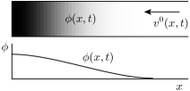
Figure 4: Sketch of the typical single-phase situation described in Sec. 3

.

In this and in the following sections we discuss several different solutions of the above model equations, which are (1) and (2), completed by the coefficient functions $q(\phi)$ and $D(\phi)$ from Eqs. (31) and (46)—Or, in their dimensionless versions, Eqs. (68), (69), (62), and (61). We here choose two functions $q(\phi)$ and $D(\phi)$ and solve the equations numerically, accompanied by analytical approximations. The aim is to display typical solutions and to explore the variety of solutions by using different functions $q(\phi)$ and $D(\phi)$. These solutions are meant to guide future experiments and their interpretation, where the final target is to employ the model for extracting the functions $q(\phi)$ and $D(\phi)$ from experimental data and to invert them to obtain the chemical potentials and the phenomenological coefficients. This will then require to solve the inverse problem of what we do in the present paper. We start with the description of three typical situations with a single phase and smooth concentration profiles, see also Fig. 4 for a sketch.

3.1 Solvent only

For setups containing only water and no solutes, the water loss is the constant $q(0)$, which has been measured experimentally by the total consumption of water per time LenJoaAjd07 . A situation with water only therefore permits to identify the constants in expression (46) for the pervaporation coefficient. A corresponding series of experiments with varying parameters can be used to verify that the assumptions we made for (46) are indeed fulfilled. Possible variations can either be geometrical such as changing the length $L$ or the height $h$ of the channel, or the membrane thickness $e$. Other variations concern the driving parameters, such as the solute concentration $\phi_{L}$ in the reservoir, or the principal control parameter during the experiment, which is the external chemical potential $\gamma_{w}^{\text{air}}$ of water in the air flow. This chemical potential is controlled by the humidity of the air circulating through the top channel. Equation (46) predicts a linear dependence of the pervaporation on the specific humidity $c_{w}^{\text{air}}$, with an offset,

$$q(0)=\frac{1}{\nu_{w}}\frac{\bar{D}}{eh}\biggl{[}\exp\Bigl{\{}\frac{m_{w}}{kT}\gamma_{w}(0)\Bigr{\}}-c_{w}^{\text{air}}\exp\Bigl{\{}\frac{m_{w}}{kT}\gamma_{w}^{\text{air}\ast}\Bigr{\}}\biggr{]},$$ (70)

where the slope of the line and the offset may in principle depend on the pressure. Quantitative information on this dependence would thus offer a validation of the current model and yield insight into the thermodynamic mechanisms inside the PDMS layer. Previous studies RanDoy05 assumed that the pervaporation is driven by a gradient of concentration and not of pressure, as we did it in Sec. 2.2.

3.2 Dilute solutions

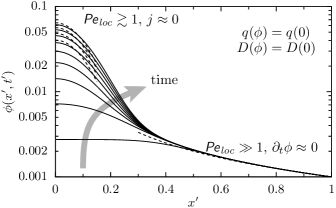
Figure 5: Growth of a dilute solute density according to the two regimes “Gaussian” and “hyperbolic ramp.” The plot shows the numerical solution with parameters ($q^{\prime}=1$, $D^{\prime}=1$, $\mbox{{Pe}}=100$, solid curves) together with the analytical approximation from Eqs. (71) and (72) (dashed curves), see also Ref. LenLonTabJoaAjd06 .

The situation with dilute solutions, in which both the evaporation coefficient $q$ and the diffusion coefficient $D$ are essentially constant, has already been explored in Ref. LenLonTabJoaAjd06 . Two different regimes were identified in the solution, first a hyperbolic ramp corresponding to a steady uniform current at high Peclet numbers, and second a Gaussian growing linearly in time, corresponding to the accumulation zone at Peclet number equal one. Both regimes can be identified in Fig. 5 where a numerical solution of equations (1) and (2) is depicted together with the analytical approximation from Ref. LenLonTabJoaAjd06 . These approximations are given by the solution of

$$\begin{gathered}j^{\prime}(1)=j^{\prime}(x^{\prime})\approx v^{0\prime}\phi=-q^{\prime}x^{\prime}\phi\\ \Longrightarrow\phi(x^{\prime})\approx-\frac{j^{\prime}(1)}{q^{\prime}x^{\prime}}\end{gathered}$$ (71)

for the hyperbolic ramp, and by the solution of

$$0=j^{\prime}(x^{\prime})=-q^{\prime}x^{\prime}\phi-\frac{D^{\prime}}{\mbox{{Pe}}}\partial_{x^{\prime}}\phi$$ (72)

for the Gaussian profile. The width of the Gaussian hump thus scales as $L/\sqrt{\mbox{{Pe}}}$. The values given in Ref. LenLonTabJoaAjd06 indicate a Peclet number of $100$.

3.3 From dilute to dense single-phase solutions

The mere model equations (1) and (2) include no mechanism to prevent unphysical values $\phi(x,t)>1$. We thus have to ask what mechanisms the model provides to ensure $\phi\leq 1$ in the dense limit when $\phi$ approaches unity. For dense solutions, both coefficients $q(\phi)$ and $D(\phi)$ exhibit non-trivial dependences on $\phi$ which provide two independent physical mechanisms to keep $\phi$ below unity. These mechanisms are described in the following paragraphs. Numerical examples for both are depicted in Fig. 6.

3.3.1 Vanishing pervaporation

One mechanism for keeping the volume fraction bounded is governed by the pervaporation coefficient $q(\phi)$. Equation (46) for this coefficient implies an equilibrium value $\phi^{\text{eq}}$ at which the pervaporation vanishes. If the concentration exceeds this value, the pervaporation direction is inverted, which stabilizes $\phi$ around the equilibrium value, see Fig. 8. In combination with the boundary condition (35) for the velocity field we find a flattening of the concentration profile at $\phi=\phi^{\text{eq}}$, at least in an interval starting with $x=0$. In this interval, the velocity remains approximately zero. A numerical example of such a profile is given in Fig. 6b.

3.3.2 Diverging diffusion coefficient

The other mechanism leading to volume fractions $\phi(x,t)$ which strictly cannot exceed unity is that the chemical potential of water diverges at $\phi\to 1$. In this case, the solvent becomes dilute in the solute, leading to the standard logarithmic form of the chemical potential of water in the solute concentration (cf. Eq. (12) or Eq. (43)). Together with the chemical potential also its derivative diverges in the limit $\phi\to 1$. In other words, the osmotic compressibility of the solute phase diverges as well: The more the solute is concentrated, the more difficult it becomes to concentrate it even further—and it cannot be concentrated beyond a value $\phi^{\text{td}}$ which is given by thermodynamics as the point where the chemical potential diverges. $\phi^{\text{td}}$ will be unity in most cases.

Mathematically speaking, the diffusive currents tend to flatten the spatial concentration profile. In the limit of an infinite diffusion coefficient—which is proportional to the derivative of the chemical potentials—the volume fraction $\phi(x,t)$ become arbitrarily flat. It will then not grow beyond the value $\phi^{\text{td}}$ at which the diffusion coefficient diverges. A numerical example for such a situation is depicted in Fig. 6a. This flattening poses a bounding mechanism which is absent if the diffusion coefficient stays finite or even vanishes.

It depends on the values of $\phi^{\text{eq}}$ and $\phi^{\text{td}}$ which of the two mechanisms takes place first in a given mixture. In the present description, however, which is based on thermodynamics, the logarithmic divergence must be located at $\phi^{\text{td}}=1$ which is always larger than the equilibrium value $\phi^{\text{eq}}$. In a mixture of small solutes, which are of molecular size, the value $\phi^{\text{td}}=1$ should indeed be approachable. It is not approachable in a system of rigid spheres in a much smaller solvent, where there is a close-packing limit $\phi^{\text{td}}<1$. In such systems with large solute particles, the solvent can still pass through the holes between the spheres, and the pervaporation never ceases footnote2 . We acknowledge that such a system cannot be described by our model—a deficiency which stems from the treatment of the pressure, and which is therefore shared by any other thermodynamic model that assumes mechanical equilibrium in form of the pressure gradient balancing all external forces. In the following, we will therefore focus the discussion on the case where the pervaporation vanishes before the diffusion coefficient diverges,

$$\phi^{\text{eq}}<\phi^{\text{td}}.$$ (73)

For our treatment of $q$ and $D$, this implies that the divergence of $D$ is not reached, because $q$ vanishes first. We thus expect the effect of drying out at least for very high densities. (Strictly speaking, this is true only for non-diverging $\mathcal{L}(\phi)$.) In dense solutions, especially at the end of the pervaporation channel, we thus expect a flat concentration profile with a nearly vanishing pervaporation and a large but finite diffusion coefficient.

We have to add a technical point here, as the diffusion coefficient depends not only on the osmotic compressibility but also on the phenomenological coefficient $\mathcal{L}(\phi)$. There are three different possibilities, which are all sketched in Fig. 8: If $\mathcal{L}(1)$ is non-zero, the diffusion coefficient diverges as $\phi\to 1$. This is the case which we have discusses so far. In the cases with vanishing phenomenological coefficient $\mathcal{L}(1)=0$ the diffusion coefficient remains finite or eventually vanishes.

Figure 6: Two different mechanisms to keep the density profile bounded from above: Panel (a) shows the influence of a diverging diffusion coefficient $D^{\prime}(\phi)=1/(1-\phi)$ while the pervaporation coefficient is constant ($q^{\prime}=1$, $\mbox{{Pe}}=10^{3}$). In this case, the velocity profile is linear for all times (not shown). In the two lower panels (b) the diffusion coefficient is constant and the pervaporation coefficient varies with $\phi$ as $q^{\prime}(\phi)=1-\phi$ ($D^{\prime}=1$, $\mbox{{Pe}}=10^{3}$). This leads to a time-dependent velocity profile.

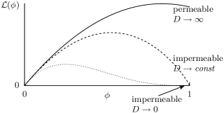
Figure 7: A sketch of the chemical potential $\gamma_{w}(\phi)$ of water with the maximal concentration permitted by thermodynamics, $\phi^{\text{td}}$. The pervaporation vanishes at the equilibrium value $\phi^{\text{eq}}$ because of the equilibrium $\gamma_{w}(\phi^{\text{eq}})=\gamma_{w}^{\text{air}}$.

Figure 8: Three possible functions $\mathcal{L}(\phi)$ for the phenomenological coefficient of inter-diffusion: They lead to qualitatively different behavior of the diffusion coefficient at $\phi\to 1$.

4 Prototype solutions: several phases

After the treatment of smooth concentration profiles such as the one in Fig. 4, we now continue with situations comprising several distinct thermodynamic phases, see Figs. 9 and 12. As more and more solute is transported from the reservoir into the channel the concentration rises and may lead to a phase transition. The position of such a phase interface and its movement in time is a convenient observable in experiments. The velocity of such an interface is governed both by the advective and the diffusive currents around it, and it thus presents a fingerprint of the mixture properties which have here been reduced to the two coefficients $D(\phi)$ and $q(\phi)$. It does not provide as much information on these coefficients as for example the full concentration profile. The interesting question is how much information on the coefficients can be extracted from the velocity of an interface as a function of time.

In addition to the model Eqs. (1) and (2) we now take the positions $X_{i}(t)$ of the interfaces into account as unknown variables. This type of problem is known as a free-surface or Stefan problem. The interface movement is governed by Eq. (39), or in its dimensionless variant by Eq. (66). The typical situation with one moving interface is sketched in Fig. 9.

4.1 Two phases: Moving phase interfaces

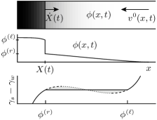
Figure 9: Sketch of the typical situation with one moving phase boundary, described in Sec. 4.1

.

To start with, we repeat the argument in Ref. LenJoaAjd07 on the experiment of solution of AOT in water. It led to an exponential decrease of the interface velocity, or equivalently to an interface position of the form

$$\frac{X(t)}{L}=1-\exp\Bigl{\{}-\frac{\phi_{L}\nu_{w}q(0)}{\Delta\phi}(t-t_{0})\Bigr{\}}$$ (74)

with an effective nucleation time $t_{0}$. This result is based on several assumptions: first, that all incoming solute current is transferred into the interface movement. This means that the total solute current $j(x,t)$ is a step-function, being zero in the dense phase (left-hand side) and a non-zero constant in the dilute phase (right-hand side). Equation (74) assumes further that the velocity profile vanishes everywhere left of the interface and that it is linear otherwise, $v^{0}(x)=-\nu_{w}q(0)\bigl{(}x-X(t)\bigr{)}$. With these two assumptions, the solute current which enters the channel at the reservoir ($x=L$) is

$$j(L,t)=\phi_{L}v^{0}(L,t)=-\nu_{w}q(0)\phi_{L}[L-X(t)].$$ (75)

The amount of solute coming from the reservoir thus depends on the position of the interface. As all solute current arrives at the phase interface, we find its movement from Eq. (66) to be

$$\dot{X}(t)=-\frac{j(X(t),t)}{\Delta\phi}=\frac{\nu_{w}q(0)\phi_{L}}{\Delta\phi}(L-X(t)).$$ (76)

This differential equation leads to the solution (74).

The two assumptions are quite strong, since the temporal change of the volume fraction $\phi$ does lead to a spatial change of solute current. Nevertheless, the solution (74) has been successfully fitted to experimental data, at least for short times. For longer times, however, it over-estimated the velocity. It is this deviation which we like to explore in the following.

For a more detailed analysis of the interface movement we have to develop a global view on the spatial solute profile. In general, whatever value the solute current has at the entrance of the channel (i. e. the concentration $\phi_{L}$ times the velocity there), it drops to zero at the end of the channel. We may therefore identify three major possible growth mechanisms due to the spatial change of the solute current along the channel: One possibility is the case we discussed around Eq. (74), where the solute current is constant in both phases with a discontinuity at the interface. The current leads to the growth of the dense phase and to the movement of the interface. The two other possibilities are losses in the bulk of the dilute and the dense phases, leading to a temporal change of the concentration profiles there.

Independent of the total solute current, the mixture velocity $v^{0}$ may be zero or not in the dense and dilute phases. In the following three subsections we discuss three different combinations of vanishing/non-vanishing currents/velocities left and right of the interface.

4.1.1 Solute accumulation at the phase boundary: the spatial profile in the dilute phase

We first investigate the spatial concentration profile which results from the assumptions taken above for Eq. (74), namely that all incoming solute is accumulated at the phase interface. The dense phase plays no role, i. e. $v^{0}(x)=0$, $j(x)=0$ for $x<X(t)$. The velocity of the interface then depends only on the concentration profile in the dilute phase,

$$\dot{X}(t)=\frac{D\partial_{x}\phi}{\Delta\phi}.$$ (77)

In a system of coordinates moving together with the interface the evolution equation for the density reads (compare with Eq. (69)),

$$\partial_{t}\phi=\dot{X}\partial_{x}\phi-\partial_{x}j.$$ (78)

A steady solution in this moving frame corresponds to a uniform current $j_{0}=-\Delta\phi\dot{X}$ in the reference frame. The uniformity of the current corresponds to the above mentioned assumption that all solute entering the dilute phase leaves it at the interface. We then find the profile stationary with respect to the moving frame as the solution of

$$(v^{0}-\dot{X})\phi-D\partial_{x}\phi=j_{0}$$ (79)

As this equation is to be solved in the dilute phase, we may assume constant coefficients $q(\phi)\approx q(0)$ and $D(\phi)\approx D(0)$ which allows to find the spatial profile

$$\phi(X(t)+y)=\exp\Bigl{\{}-\Bigl{(}\frac{y+\beta}{\alpha}\Bigr{)}^{2}\Bigr{\}}\times\\ \biggl{[}\phi^{(r)}\exp\Bigl{\{}\frac{\beta^{2}}{\alpha^{2}}\Bigr{\}}+2\Delta\phi\frac{\beta}{\alpha}\Bigl{[}G\Bigl{(}\frac{y+\beta}{\alpha}\Bigr{)}-G\Bigl{(}\frac{\beta}{\alpha}\Bigr{)}\Bigr{]}\biggr{]},$$ (80)

with the shortcuts

$$\alpha:=\sqrt{\frac{2D}{\nu_{w}q}}=L\,\sqrt{\frac{2}{\mbox{{Pe}}}},\quad\beta:=\frac{\dot{X}}{\nu_{w}q},\quad G(x):=\int_{0}^{x}e^{\xi^{2}}d\xi.$$ (81)

Figure 10: Visualization of the solution (80) which is stationary in the frame moving with the interface. The parameters are arbitrary ($\mbox{{Pe}}=10^{3}$, $\dot{X}^{\prime}=0.05$, $\phi^{(r)}=0.3$, $\phi^{(\ell)}=0.8$).

An example of this solution is shown in Fig. 10. It exhibits the same two regimes as the dilute equation described above in Sec. 3.2 and in Fig. 5: There is a hump dominated by diffusion and a hyperbolic ramp.

The solution from Eq. (80), depicted in Fig. 10 gives insight into the implications of the taken assumptions: It shows that the diffusive hump exceeds the binodal concentration value $\phi^{(r)}$. Evidently, there is a zone of higher concentration which moves together with the phase interface, and which continuously feeds the dense phase. As long as both the velocity and the total solute current vanish at the interface, the diffusive hump must exceed the value $\phi^{(r)}$ since there must be a negative current causing the interface to move to the right. The only contribution to the solute current is the one caused by the concentration gradient, thus having to be positive. The assumptions $j(X,t)=0$ and $v^{0}(X,t)=0$ create a situation in which it is in principle possible that the peak which is clearly visible in Fig. 10 reaches a spinodal value, which is larger than $\phi^{(r)}$ but smaller than $\phi^{(\ell)}$. As the concentration reaches the spinodal, it will undergo local phase changes and exhibit local blobs of a metastable phase. Such blobs have occasionally been observed in the experiments using a KCl solution LenLonTabJoaAjd06 .

The diffusive hump in Fig. 10 appears pronounced due to the large Peclet number chosen in this example. The Peclet number renders the length scale $\alpha$ small, which reduces the lateral extension of the hump and increases its maximum value. In experimental realizations, its height is limited by several factors, first by the overall Peclet number, second by the spinodal concentrations which enforce a local phase transition instead of the smooth maximum, and third by the pervaporation in the dense phase. For a non-vanishing velocity $v^{0}(X,t)$ the necessity of having a positive slope $\partial_{x}\phi$ at $x=X(t)$ gradually vanishes, allowing the height of the maximum to decrease or to vanish completely.

We continue to discuss the solution (80) by showing how the result (74) follows from the spatial form of the solute concentration. The hyperbolic ramp, which is the asymptotic solution for large $x$, here reads (in rescaled units)

$$\phi(X(t)+y)\sim\frac{\Delta\phi}{1+y^{\prime}/\dot{X}^{\prime}}.$$ (82)

We may use the asymptotic form to calculate an approximate velocity of the interface: Of course, this result corresponds to a stationary solution in a reference frame moving at constant velocity. Therefore, the input concentration at the end of the channel must be increased consistently in order to find this solution. Reversely, if the input concentration is held constant at $\phi(L)=\phi_{L}$, the current arriving at the phase interface decreases in time. As long as the diffusive hump does not reach the inlet of the channel, this change of current is small and we may use $\phi(L)$ as a slowly varying parameter. Setting $\phi(L)=\phi_{L}$ in the asymptotic solution (82) then yields essentially the same expression for the evolution of the interface position as in equation (74),

$$X^{\prime}(t)=1-\exp\Bigl{\{}-\frac{\phi_{L}}{\Delta\phi-\phi_{L}}(t^{\prime}-t^{\prime}_{0})\Bigr{\}}.$$ (83)

4.1.2 Solute accumulation at the phase boundary: the velocity field in the dense phase

As a next approximation we relax the assumption of a vanishing velocity left of the interface. However, we continue to keep the total current zero in the dense phase. Also the dilute phase is passive, such that all incoming solute is accumulated at the interface.

As discussed above in section 3.3 the velocity and density profiles in dense phases can behave in two qualitatively different ways: One corresponds to the vanishing of $q(\phi)$ and the other to the divergence of $D(\phi)$. We make the same distinction here. The first case, with vanishing $q(\phi)$, is characterized by a flat velocity profile near the end of the channel. It is likely to lead to a density profile which has maximum density from the end of the channel up to the interface, where it reaches a small region with non-vanishing velocity. After a transient time, the density profile in a small region could become stationary in a reference frame moving together with the interface. This solution supports a mixture velocity at the interface that is constant in time. The position of the interface is then given by

$$\frac{X(t)}{L}=\Bigl{(}1-\frac{v(X)}{L\nu_{w}q(0)}\Bigr{)}\Bigl{(}1-\exp\Bigl{\{}-\frac{\phi_{L}\nu_{w}q(0)}{\Delta\phi}(t-t_{0})\Bigr{\}}\Bigr{)}.$$ (84)

The dilute phase is here characterized by a constant $q$ and $D$.

In the second case, in which the diverging diffusion coefficient leads to a bounded density profile, the velocity field needs not to vanish except at the very end of the channel. For simplicity, we adopt a constant non-zero value for the pervaporation in the dense phase, $q(\phi)\approx q(1)<q(0)$. This solution leads to a piecewise linear mixture velocity and to the interface position

$$\frac{X(t)}{L}=\frac{q(0)}{q(0)-q(1)}\Bigl{(}1-\exp\Bigl{\{}-\frac{\phi_{L}\nu_{w}q(0)}{\Delta\phi}(t-t_{0})\Bigr{\}}\Bigr{)}.$$ (85)

None of the solutions (84) and (85) can explain the velocity decrease found in the AOT experiments. Instead, both velocities are larger than the initial proposition solution (74). Note that we still kept the assumption $j(x)=0$ in the dense phase, which corresponds to a large diffusion coefficient. It must therefore be concluded that in the case of AOT either the diffusion coefficient is not sufficiently large, or the velocity decrease stems from the dilute phase.

4.1.3 Solute accumulation also in the dilute phase

In both preceding subsections we have kept the assumption that all incoming solute contributes to the movement of the interface. We now continue with the more general case where there may be a temporal change of the concentration profile such that there is a gradient of solute current in the dilute phase. The dense phase is still assumed to be passive (no pervaporation).

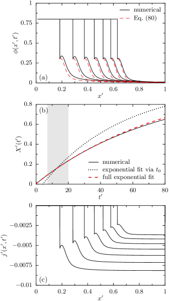
Figure 11: Numerically determined density profile $\phi(x^{\prime},t^{\prime})$ containing a single moving phase interface. The binodal density values at the interface are $\phi^{(\ell)}=0.8$ and $\phi^{(r)}=0.3$; at the channel entry $\phi_{L}=10^{-2}$; $\mbox{{Pe}}=10^{3}$. Panel (a) shows the density profile, panel (b) the position of the interface as a function of time, and panel (c) the evolution of the spatial current profile.

This more general situation cannot be described analytically but has to be treated numerically. A numerical test of the situation with a dense phase growing into a dilute one exhibits the limitations of the assumption taken above in Sec. 4.1.1. Figure 11 shows the full numerical solution of the model. The velocity in the dense part has been kept zero ($q=0$), leading to a flat density profile there. The dilute part of the solution agrees qualitatively with the graph given in Fig. 10. There are, however, deviations. The plot shows the solutions of Eq. (80) with the true position and the true velocity of the interface taken from the numerical solution. Panel b quantifies the difference between the approximation from Sec. 4.1.1 and the true solution. It shows the position of the interface as a function of time. A fit with the exponential function (74) with the known value for $\phi_{L}\nu_{w}q/\Delta\phi$ and $t_{0}$ as the fitting parameter proves that the approximation does not work in this example. A second fit for both parameters indicates that the resulting function is still exponential, but with a different timescale than assumed in the approximation (74). In both fittings only the data in the gray-shaded area has been used. The fit quantifies that around $60\%$ of the incoming solute is accumulated at the interface and leads to the growth of the dense phase. The rest remains in the dilute phase. Panel 11c visualizes this ratio directly. Evidently, the current has not the form of a step function, but takes on different values at the interface and at the channel entry. This clearly falsifies the assumption of a uniform current in the dilute phase.

Upon varying the parameters of the example, we found that the concentration $\phi^{(r)}$ right of the interface has the largest influence on the deposition of current. For $\phi^{(r)}=0.05$ nearly all of the incoming current was found to accumulate at the phase boundary—despite a well developed diffusive hump similar to the one in Fig. 11a, and despite the fact that the solute current still exhibited a pronounced hump. The current apparently overflows the diffusive hump completely, if $\phi(x,t)$ has already reached the value $\phi^{(r)}$ before the hump starts. We may quantify this by stating that approximation (74) is valid if

$$\phi^{(r)}\leq\sqrt{\mbox{{Pe}}}\>\frac{L-X}{L}\>\phi_{L}.$$ (86)

Here, we assumed the width of the diffusive hump to scale as $L/\sqrt{\mbox{{Pe}}\,}$, see the definition of $\alpha$ in (81), and also Ref. LenLonTabJoaAjd06 .

4.2 Several phases: Phase slab thicknesses in stationary solutions

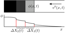
Figure 12: Sketch of the situation with several phase slabs exhibiting characteristic extents, as described in Sec. 4.2

.

We now return to the introductory example of Sec. 1.2 with four phases, one of them dilute. This situation is sketched in Fig. 12. The aim here is to present an example how the thicknesses of phase slabs are governed by the thermodynamic and dynamic properties of all the phases.

For the solution of AOT in water, a remarkable observation has been reported in Ref. LenJoaAjd07 : First, the same phases as in equilibrium have been found in the evaporation channel. They were identified by their polarizability and birefringence, showing hexagonal, cubic and lamellar internal structures for the dense phases, while the dilute phase was isotropic. The spatial pattern showed that the two enclosed slab thicknesses (of the cubic and the lamellar phases) were of comparable extension. This result is remarkable because these two phases occupy a very different range of $\phi$-values in the equilibrium phase diagram. There, the lamellar phase appears much broader than the cubic phase, see the supplementary material of Ref. LenJoaAjd07 . We conclude that there is apparently a much larger concentration gradient in the lamellar phase than in the cubic phase. This larger concentration gradient was stable in the experiment, even when all dense phases were continuously fed with more incoming solute. After a short transient time, the interfaces bounding the cubic and the lamellar phase moved together at constant distance.

We now show that our model possesses qualitatively the same solutions. We also observe stable thicknesses of comparable size for the lamellar and the cubic phases, if we choose the chemical potential and the phenomenological coefficients well. The strategy here is to adopt simple model functions for $\gamma_{w}(\phi)$ and $\mathcal{L}(\phi)$. They are then transferred into diffusion coefficient $D(\phi)$ and pervaporation coefficient $q(\phi)$ using Eqs. (61) and (62) which are then used in the stationary model equations.

We here adopt the most simple models for the chemical potential and for the phenomenological coefficients. The functions used below are displayed in Fig. 14. The values of $\phi$ are taken from the equilibrium phase diagram of AOT (see supplementary material of Ref. LenJoaAjd07 ). The regions shaded in gray indicate phase coexistence, where the chemical potentials are constant. Within the most dense phase we use a logarithmic behavior of the form $\gamma^{\prime}_{w}(\phi)\propto\ln(1-\phi)$, whereas in the other three phases we linearly connect some coexistence values which have been chosen as model parameters. The phenomenological coefficient has been chosen constant in each phase except in the dilute phase where a linear function of $\phi$ is required (see Sec. 2.3.2). The coefficients $q^{\prime}(\phi)$ and $D^{\prime}(\phi)$ follow from equations (61) and (31), see Fig. 14.

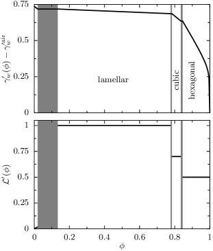
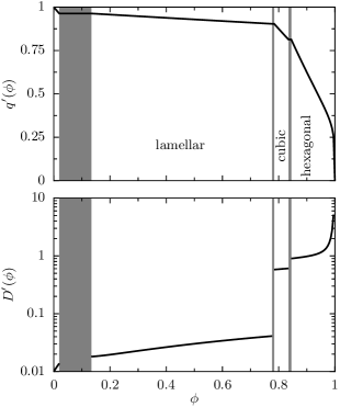
Figure 13: Simple model functions for the rescaled chemical potential difference of water across the PDMS layer and for the phenomenological coefficient, both as functions of the volume fraction $\phi$. Note the different slopes of the chemical potential in the lamellar and the cubic phases which lead to the same slab thickness in Fig. 16.

Figure 14: The rescaled coefficients for evaporation $q^{\prime}(\phi)$ and for diffusion $D^{\prime}(\phi)$ resulting from the model in Fig. 14.

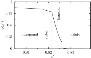
Figure 15: An example solution of the stationary equations in which the thickness of phase slabs is controlled by the slope of chemical potential in Fig. 14. Note the equal thickness of the lamellar and the cubic phases.

Figure 16: The development of phase thicknesses for (a) the model given in Fig. 14; and in (b) for a chemical potential in the cubic phase having the same slope as the one in the lamellar phase.

Figure 16 shows a typical profile of the volume fraction of solute, $\phi(x^{\prime})$, as it results from the model functions given in Figs. 14 and 14. The lamellar and cubic phases are indeed found to have approximately the same extent. It is mainly the different slope of the chemical potential in Fig. 14a which has been adjusted manually to achieve the comparable extent of the two phases. The physical content of these slopes are the very different osmotic compressibilities of these two phases. Of course, also the phenomenological coefficient plays a role. We do not claim that the presented chemical potentials are the only ones which may lead to comparable phase extensions. However, it is evident in this very example that the osmotic compressibilities of the chemical potential directly influence the extension of the phase slabs. The profile in Fig. 16 has been calculated as the stationary solution of the model equations (56) and (57). The use of the stationary equations will be explained in the following.

4.2.1 Stationary and quasi-stationary solutions

The full evolution of the phase thicknesses in time is subject to many parameters including not only the model parameters for $D(\phi)$ and $q(\phi)$ and the incoming volume fraction and the Peclet number. It depends also on the initial state, or in other words, on the precise conditions of phase creation at the end of the channel. We do not want to treat the issues of phase creation here, the more as a reasonably fast numerical method for this parameter regime is not at hand. Instead, we employ a quasi-stationary treatment, which is focused on the main features of the phase thicknesses. The idea is to assume a very small input current and to assume at any time an equilibrated stationary profile. Such a stationary profile is shown in Fig. 16 for the model functions of Fig. 14. Note the slab thicknesses of the lamellar and the cubic phases which are of the same extent. This behavior has been achieved by choosing the slopes of the chemical potential in Fig. 14, which is $20$ times larger in the cubic phase than in the lamellar one. Of course, the variation of the chemical potential also has its influence on the evaporation. We thus cannot clearly separate between thickness due to a variation of diffusion and due to modified pervaporation. This ambiguity is a systematic issue in the interpretation of the experimental results, and it is reflected in our model by the two coefficients $D$ and $q$.

In order to obtain the ensemble of all boundary positions, which is given in Fig. 16, we parametrized the solutions by the total amount of solute $\int\phi(x^{\prime})\,dx^{\prime}$. In a quasi-stationary setting with extremely small input current, this amount may be understood as time multiplied by the input current. A numerical test of the full time-dependent equations revealed similar lines as a function of time (not shown). It can be seen that the interior slab thicknesses relax to constant values, and that only the last, the hexagonal phase continues to grow. This behavior stems from the vanishing pervaporation in the hexagonal phase which leads at the interfaces to a mixture velocity constant in time. If the velocity does not vanish in the dense phase, then the interior thicknesses do not truly become stationary.

In order to demonstrate the effect of the slopes of the chemical potential on the slab thicknesses, Fig. 16b presents the result for a modified model chemical potential. We took the curve in Fig. 14a and changed the slope in the cubic phase to the slope in the lamellar phase. This situation implies the same osmotic compressibilities in both phases, and also a comparable spatial concentration gradient. As a result, the cubic phase has shrunk and is hardly visible in Fig. 16b.

The numerical solutions in Figs. 16 and 16 have been created by a Runge–Kutta algorithm solving the stationary equations (1) and (2). On the analytical side, they may be solved formally by integration over $\phi$. The stationary equations can be rewritten such that

$$\frac{d}{dx}(v^{0})^{2}=-\frac{D(\phi)\partial_{x}\phi}{\phi}\nu_{w}q(\phi)\quad\text{and}$$ (87)

$$\frac{dx}{d\phi}=\frac{D(\phi)}{v^{0}\phi}.$$ (88)

The formal solution of the problem then reads

$$v^{0}(x,x_{0})=-\biggl{[}{\textstyle\bigl{(}v^{0}(x_{0})\bigr{)}^{2}+2\nu_{w}\int\limits_{\phi(x)}^{\phi(x_{0})}\frac{D(\xi)q(\xi)}{\xi}d\xi}\biggr{]}^{\frac{1}{2}}$$ (89)

$$x=x_{0}+\int\limits_{\phi(x)}^{\phi(x_{0})}\frac{D(\varphi)}{\varphi}\biggl{[}{\textstyle\bigl{(}v^{0}(x_{0})\bigr{)}^{2}+2\nu_{w}\int\limits_{\varphi}^{\phi(x_{0})}\frac{D(\xi)q(\xi)}{\xi}d\xi}\biggr{]}^{-\frac{1}{2}}d\varphi.$$ (90)

This expression describes in principle any stationary solution, but in the unusual way $x(\phi)$. This formulation is especially convenient for the determination of phase slab thicknesses. For the first phase at the end of the evaporation channel, the expression simplifies due to the boundary condition $v^{0}(0)=0$. In case of the phase interface $x=X(t)$ the lower bound of the integrals is fixed to the binodal value $\phi^{(\ell)}$ of the phase transition. We then find

$$v^{0}(X(t))=-\biggl{[}{2\nu_{w}\int_{\phi^{(\ell)}}^{\phi(0,t)}\frac{D(\xi)q(\xi)}{\xi}d\xi}\biggr{]}^{\frac{1}{2}}$$ (91)

$$X(t)=\int_{\phi^{(\ell)}}^{\phi(0,t)}\frac{D(\varphi)}{\varphi}\biggl{[}{2\nu_{w}\int_{\varphi}^{\phi(0,t)}\frac{D(\xi)q(\xi)}{\xi}d\xi}\biggr{]}^{-\frac{1}{2}}d\varphi$$ (92)

4.2.2 Phase nucleation

The treatment of the phase thickness in the present section resembles to some extent the treatment of nucleation as it has been presented by Evans, Poon, and Cates EvaPooCat97 . Both include the assumption of local equilibrium, leading to a diffusion-type equation, while the total system is out of equilibrium. Both allow the occurrence of metastable phases which are absent in equilibrium. Here, these phases are the dense ones growing because of the non-zero solvent flow; in Ref. EvaPooCat97 it is a freshly nucleated metastable phase which grows because the whole system is quenched in temperature.

We have not included the details of phase nucleation near the end of the channel, as it would require a more advanced numerical treatment. The general framework, however, should be applicable to the nucleation in a similar manner as in Ref. EvaPooCat97 .

5 Summary

We have derived a model for the behavior of binary solute–solvent mixtures in recently developed microevaporator devices. The final target of the model is to allow an interpretation of experimentally observed data in terms of well-defined thermodynamic and dynamic properties of the mixture which are measurable also by different means. As a first step towards this goal we have developed the model equations (1) and (2) which relate the phase behavior in the microevaporator to an inter-diffusion coefficient $D$ and another coefficient $q$ quantifying the pervaporation of solute. We have shown in Eqs. (31) and (46) how these two coefficients depend on the chemical potentials in the mixture and on the phenomenological coefficient for inter-diffusion. This relation has then been extended to make also the connection to other quantities such as the coefficients of sedimentation, permeability and osmotic compressibility.

The presented model is focused on the transport equations of solute and solvent mass in binary mixtures, using the hypothesis of local thermodynamic equilibrium. We provide in detail all the necessary assumptions to reduce the description to two variables, one of which is the volume fraction of solute, the other one is the volume-averaged mixture velocity. We further assume incompressibility of the mixture and reduce the spatial dimensions to the one parallel to the evaporation channel.

We solved the model equations in a number of typical limit cases which still allow analytical approximations and compared these with full numerical solutions. In particular we found good agreement in the case of dilute solutions, where the diffusion and pervaporation coefficients may be treated as constants. In dense binary mixtures, where this is no longer the case, we were able to show that there are two qualitatively different mechanisms which both lead to a saturation of the concentration at its maximal possible value. One of them is due to vanishing evaporation at an equilibrium concentration. The other case comes from the singular behavior of the chemical potential of water in this limit.

We have further analyzed the growth velocity of a dense phase into a dilute one and have found several expressions which allow to extract quite some information on the properties of the mixture only from tracking a single interface between two phases. Further, we have analyzed the resulting thicknesses of phase slabs in the microevaporator in a stationary setting. In particular, the experimentally observed case of equal phase thicknesses has been regarded. We were able to explained this remarkable fact as the result of very different osmotic compressibilities in the two phases.

In total, the results presented here show that the interpretation of the experimental results is possible but far from trivial. In all cases, there is some ambiguity in the interpretation of the observed behavior: As the physical properties of the mixture are summarized in two coefficients, also the reasons for the flattening at high solute concentrations are twofold. In a similar manner, the thicknesses of the phase slabs are not only governed by their thermodynamic properties, but also by the phenomenological coefficient containing dynamic information.

It is precisely this twofold information contained in the microevaporator data as well as in the two coefficients $D$ and $q$ which presents the core of the present work. We are convinced that the presented model establishes a good first compromise between the complexity of the phenomenon being out of equilibrium and the need for simplicity in the equations. Our model will help on the experimental plan to identify sets of measurements which allow to lift the ambiguity in the coefficients. It is the detailed derivation of the model and the numerical treatment of the equations which allows to improve the interpretation of the experimentally measured quantities and to extract from them the chemical potentials and the transport coefficients as full functions of the solute concentration.

Acknowledgements: We are grateful to J. Leng for valuable discussions on the experiments. For comments on the manuscript we thank K. Sekomoto and D. Lacoste. This work was financed by the German DFG via grant Schi/1-1 and by the French ANR via project “Scan 2”.

References

- (1) W. Machtle, in: S. E. Harding, A. J. Rowe, J. C. Horton (Eds.), Analytical Ultracentrifugation in Biochemistry and Polymer Science (The Royal Society of Chemistry, Cambridge 1992) 147–175.
- (2) Q. G. Wang, H. D. Tolley, D. A. LeFebre, and M. L. Lee, Anal. Bioanal. Chem. 373, (2002) 125.
- (3) W. B. Russel, D. A. Saville, and W. R. Schowalter, Colloidal Dispersions (Cambridge University Press, Cambridge, 1989).
- (4) S. S. L. Peppin, J. A. W. Elliot, and M. G. Worster, Phys. Fluids 17, (2005) 053301.
- (5) J. Lebowitz, M. S. Lewis, P. Schuck, Protein Sci. 11, (2002) 2067.
- (6) D. R. Paul, J. Membrane Sci. 241, (2004) 371.
- (7) J. Leng, B. Lonetti, P. Tabeling, M. Joanicot, and A. Ajdari, Phys. Rev. Lett 96, (2006) 084503.
- (8) J. Leng, M. Joanicot, and A. Ajdari, Langmuir 23, (2007) 2315.
- (9) J.-B. Salmon, J. Leng, to appear.
- (10) J. Shim, G. Cristobal, D. R. Link, T. Thorsen, Y. Jia, K. Piattelli, and S. Fraden, J. Am. Chem. Soc. 129, (2007) 8825.
- (11) B. T. C. Lau, C. A. Baitz, X. P. Dong, and C. L. Hansen, J. Am. Chem. Soc. 129, (2007) 454.
- (12) S. R. de Groot and P. Mazur, Non-Equilibrium Thermodynamics (Dover Publications, New York 1984).
- (13) D. D. Joseph, A. Huang, and H. Hu, Physica D 97, (1996) 104.
-
(14)
The comparison of the two terms in Eq. (29) requires
several individual estimations: (A) The pressure gradient is approximated by
the one in a Poiseuille flow in the same rectangular channel. This should be a
good approximation for a dilute solution at the entrance of the channel near
the reservoir. We take typical values from Ref. LenLonTabJoaAjd06 ,
namely , , , together with the
viscosity of water, . This leaves us with a
pressure gradient of
with the shape-factor taken from Ref. MorOkkBru05 . As a further approximation (B) we take the chemical potentials in their dilute limit, where becomes logarithmic in , yielding(93)
We also anticipate (C) the “hyperbolic ramp” solution at the entrance of the channel (see Sec. 3.2 and Ref. LenLonTabJoaAjd06 for an experimental evidence), . This approximation leaves us with the concentration gradient of the order . Putting all pieces together, the ratio of the two terms in Eq. (29) is(94)
If we say that the solute is ten times lighter than the solvent water (approximation D), the difference of specific volumes will be dominated by that factor. Together with a molecular weight of a few hundred atom units, we end up with the factor in Eq. (95) to be less than , which justifies the approximation in Sec. 2.1.4.(95) - (15) W. H. Press and S. A. Teukolsky and W. T. Vetterling and B. P. Flannery, Numerical Recipes in C (Cambridge University Press, Cambridge 1992).
- (16) G. C. Randall, P. S. Doyle, Proc. Natl. Acad. Sci. USA. 102, (2005) 10813.
- (17) The pervaporation may cease if the spheres exhibit some compressibility which enters the chemical potential.
- (18) R. M. L. Evans, W. C. K. Poon and M. E. Cates, Europhys. Lett. 38, (1997) 595.
- (19) N. A. Mortensen, F. Okkels, and H. Bruus, Phys. Review E 71, (2005) 057301.