A novel changepoint detection algorithm

Abstract

We propose an algorithm for simultaneously detecting and locating changepoints in a time series, and a framework for predicting the distribution of the next point in the series. The kernel of the algorithm is a system of equations that computes, for each index $i$, the probability that the last (most recent) change point occurred at $i$. We evaluate this algorithm by applying it to the change point detection problem and comparing it to the generalized likelihood ratio (GLR) algorithm. We find that our algorithm is as good as GLR, or better, over a wide range of scenarios, and that the advantage increases as the signal-to-noise ratio decreases.

1 Introduction

Predicting network performance characteristics is useful for a variety of applications. At the protocol level, predictions are used to set protocol parameters like timeouts and send rates [11]. In middleware, they are used for resource selection and scheduling [14]. And at the application level, they are used for predicting transfer times and choosing among mirror sites.

Usually these predictions are based on recent measurements, so their accuracy depends on the constancy of network performance. For some network characteristics, and some time scales, Internet measurements can be described with stationary models, and we expect simple prediction methods to work well. But many network measurements are characterized by periods of stationarity punctuated by abrupt transitions [15] [9]. On short time scales, these transitions are caused by variations in traffic (for example, the end of a high-throughput transfer). On longer time scales, they are caused by routing changes and hardware changes (for example, routers and links going down and coming back up).

These observations lead us to explore statistical techniques for changepoint detection. Changepoint analysis is based on the assumption that the observed process is stationary during certain intervals, but that there are changepoints where the parameters of the process change abruptly. If we can detect changepoints, we know when to discard old data and estimate the new parameters.

Thus, changepoint analysis can improve the accuracy of predictions. It can also provide meta-predictions; that is, it can be used to indicate when a prediction is likely to be accurate.

Statisticians have done extensive work on the general problem of changepoint detection. Variations on the changepoint problem [2] include:

Changepoint detection:

The simplest version of the changepoint problem is testing the hypothesis that a changepoint has occurred. Elementary algorithms for change detection include control charts, CUSUM algorithms and likelihood ratio tests [1].

Location estimation:

For some applications it is important to estimate the location (time) of the changepoint. More generally, it might be useful to find a confidence set or an interval of times that contain a changepoint at some level of confidence.

Tracking:

The goal of the tracking problem is to partition a time series into stationary intervals and estimate the parameters of the process in each interval. A simple approach is to use hypothesis testing to detect a changepoint, estimate the location of the change(s), and then use conventional techniques to estimate the parameters of the process in each interval.

For each of these problems, there is an alternative Bayesian formulation. Instead of testing (and possibly rejecting) the hypothesis that a changepoint has occurred, the Bayesian approach is to compute the subjective probability of the hypothesis. Instead of estimating the location, the Bayesian approach is to compute $P(i)$, the probability that there is a changepoint at index $i$. The Bayesian version of the tracking problem is to compute the probability of a changepoint at a given time and the conditional distribution of the parameters (conditioned on the location).

In this paper, we take the Bayesian approach and apply it to the tracking problem. Our algorithm can also be used for changepoint detection and location estimation.

1.1 Online or off?

Changepoint detection algorithms are sometimes classified as “online” or “offline”, but this is not an intrinsic characteristic of the algorithm; it is a description of the deployment. Online algorithms run concurrently with the process they are monitoring, processing each data point as it becomes available, with the real-time constraint that processing should complete before the next data point arrives. Offline algorithms consider the entire data set at once, and there is no real-time constraint on the run time.

So in most cases, “online” means “fast enough to keep up”. Sometimes it means “incremental”, in the sense that when a new data point arrives, the algorithm can perform an update, based on previously stored results, faster than it could recompute from scratch. Incremental algorithms are particularly appealing in embedded applications, where processing power is at a premium, but it is not generally necessary for online algorithms to be incremental.

“Online” and “offline” are probably best used to describe the problem formulation rather than the algorithm. In the online scenario, the goal is to detect a changepoint as soon as possible after it occurs, while minimizing the rate of false alarms. In the offline scenario, the goal is often to identify all changepoints in a sequence, and the the criteria are sensitivity (detecting true changepoints) and specificity (avoiding false positives).

The algorithm we are proposing can be used for both online and offline problems. It is incremental, so it lends itself to online deployment; on the other hand, it requires computation time proportional to $n^{2}$ for each data point, where $n$ is the number of points in the current window, so for some applications it may not be fast enough to satisfy real time requirements.

Nevertheless, since the applications we are considering (making real time predictions) are online, we evaluate our algorithm by the criteria of online problems.

1.2 Prediction with changepoints

The goal of this work is to generate a predictive distribution from a time series with changepoints. For example, imagine that we have observed $n$ values $x_{1}\ldots x_{n}$, and we want to predict the value of $x_{n+1}$. In the absence of changepoints, we might model the series as a random variable $X$ with a stationary distribution (and, possibly, autocorrelation structure). We could use the observed values to estimate the parameters of $X$ and then use those parameters to compute the distribution of the next value.

If we know that there is a changepoint, and we assume that there is no relation between the parameters of the process before and after the change, then the data before the changepoint are irrelevant for making predictions.

But in the context of network measurements, we usually don’t know when a changepoint occurs. We can only infer it from the time series itself, and we usually don’t know with certainty whether it occurred or exactly when.

There are two ways to handle this uncertainty. The most common approach is to compute from the data a functional that is likely to increase after a changepoint and to compare the resulting values to a previously-chosen threshold. If the value exceeds the threshold, we assume that there was a changepoint and discard older data. Otherwise we assume that there was no changepoint.

The alternative, which we explore here, is to use changepoint probabilities to generate predictive distributions. For example, if we think that there is $p$ chance of a changepoint at $i$, then we can generate two distributions, one that assumes that there was a changepoint, and one that assumes that there wasn’t, and then mix the distributions using $p$ as a weight.

Therefore, our intermediate goal is to compute $P(i^{+})$, which we define as the probability that $i$ is the index of the last (most recent) changepoint. The $+$ notation is intended to distinguish from $P(i)$, which is the probability that $i$ is the index of a changepoint (but not necessarily the last).

1.3 Related Work

In a seminal paper on the tracking problem, Chernoff and Zacks present a Bayesian estimator for the current mean of a process with abrupt changes [4]. Like us, they start with an estimator that assumes there is at most one change, and then use it to generate an approximate estimator in the general case. Their algorithm makes the additional assumption that the change size is distributed normally; our algorithm does not require this assumption. Also, our algorithm generates a predictive distribution for the next value in the series, rather than an estimate of the current mean.

Since then, there has been extensive work on a variety of related problems, using both Bayesian and non-Bayesian approaches. More recent works include extensions to deal with multiple changepoints, autoregressive processes, and long-range dependent processes.

The algorithm we propose can be extended to detect changes in the variance as well as the mean of a process. This kind of changepoint has received relatively little attention; one exception is recent work by Jandhyala, Fotopoulos and Hawkins [8].

Most recently, Vellekoop and Clark propose a nonlinear filtering approach to the changepoint detection problem (but not estimation or tracking) [13].

We are aware of a few examples where these techniques have been applied to network measurements. Blažek et al explore the use of change-point algorithms to detect denial of service attacks [3]. Similarly Deshpande, Thottan and Sikdar use non-parametric CUSUM to detect BGP instabilities [6].

In the context of large databases, Kifer, Ben-David and Gehrke propose an algorithm for detecting changes in data streams [10]. It is based on a two-window paradigm, in which the distribution of values in the current window is compared to the distribution of values in a past reference window. This approach is appropriate when the number of points between changepoints is large and alarm delay is not a critical metric.

1.4 Outline

Before presenting our algorithm we provide a summary of the techniques and results we will use from Bayesian statistics (Section 2). Then we develop our algorithm, starting with a direct method for the case where we know there is exactly one changepoint, and then using that result to develop an iterative method for the case where the number of changepoints is unknown (Section 3). That section includes synthetic examples to demonstrate changes in both mean and variance, and one real series, the ubiquitous Nile dataset. Finally, we apply our algorithm to the changepoint detection problem and compare it with GLR, a standard algorithm for this problem (Section 4).

2 Bayesian Statistics

This section presents an introduction to Bayesian statistics, and develops several examples we will use in later sections.

The fundamental idea behind all Bayesian statistics is the diachronic interpretation of Bayes’ Theorem:

$$P(H|E)=\frac{P(E|H)P(H)}{P(E)}$$ (1)

where $H$ is a hypothesis and $E$ is a relevant body of evidence. $P(H|E)$ is the probability of the hypothesis given the evidence, which is called the posterior probability. $P(H)$ is the probability of the hypothesis before we take account of the evidence, known as the prior probability. $P(E|H)$ is the probability of seeing the evidence, given that the hypothesis is true; this term is sometimes called the likelihood. Finally, $P(E)$ is the probability of seeing the evidence under any possible hypothesis, called the normalizing constant.

If the hypotheses we are interested in are stochastic processes, it is usually straightforward to compute $P(E|H)$. The prior probability $P(H)$ is either based on a previous computation or reflects a subjective degree of belief in the hypothesis before seeing the evidence. The normalizing constant is hard to formulate in general, but if we can identify a mutually exclusive and complete set of hypotheses, S, then

$$P(E)=\sum_{H_{i}\in S}P(E|H_{i})P(H_{i})$$ (2)

In practice it is sufficient to compute any likelihood function, $L(E|H)$, such that

$$L(E|H)=\kappa P(E|H)P(H)$$ (3)

where $\kappa$ is an arbitrary constant that drops out when we compute

$$P(H|E)=\frac{L(E|H)}{\sum_{H_{i}\in S}L(E|H_{i})}$$ (4)

As an example, suppose that $H$ is the hypothesis that a random variable $X$ is distributed $N(\mu,\sigma^{2})$ with known $\mu$ and $\sigma^{2}$. In a continuous distribution, the probability of a given selection $X=x$ is not well defined, but since the probability density function $pdf_{X}(x)$ is proportional to $P(X=x|H)$, we can use it as a likelihood function:

$$L(X=x|H)=pdf_{X}(x)=\\ \frac{1}{\sigma\sqrt{2\pi}}\exp\left[-\frac{1}{2}\left(\frac{x-\mu}{\sigma}\right)^{2}\right]$$ (5)

For a sample $E=x_{i}$ with $i=1\ldots n$

$$L(E|H)=\prod_{i}pdf_{X}(x_{i})$$ (6)

2.1 Posterior distributions

We have been using the notation $P(A)$ to mean the probability of an event $A$. Following the notation of Gelman et al [7], we use $p(x)$ as a shorthand for the probability density function $pdf_{X}(x)$. This notation makes it convenient to write Bayes’ Theorem for distributions. For example, if we observe a set of data, $y$, we might want to compute the distribution of $\theta$, which is the set of parameters of the process that produced $y$. Generalizing Bayes’ Theorem yields

$$p(\theta|y)=\frac{p(y|\theta)p(\theta)}{p(y)}$$ (7)

where $p(\theta)$ is the prior distribution of $\theta$, and $p(\theta|y)$ is the posterior distribution.

As an example, suppose that $y$ is a set of interarrival times between passengers at a bus stop, and the arrival process is Poisson; in this case $\theta$ is the single parameter of the Poisson model (the mean arrival rate), and $p(\theta|y)$ is the distribution of $\theta$, taking the observed data into account. In frequentist statistics, $\theta$ is not a random variable, so it is not meaningful to talk about its distribution, but in the Bayesian interpretation, probability can reflect a degree of belief about a non-random quantity.

As another example, which we will use in Section 3, suppose that we have a set of observations $y$ that come from a normal distribution with unknown mean $\mu$ and variance $\sigma^{2}$. We would like to compute posterior distributions for $\mu$ and $\sigma$. For this problem it is common to use a noninformative prior distribution that is uniform on ($\mu$, $\log(\sigma)$), in which case the posterior distribution of $\sigma^{2}$ is a scaled inverse chi-square distribution:

$$\sigma^{2}|y\sim\mbox{Inv-}\chi^{2}(n-1,s^{2})$$ (8)

where $n$ is the number of observations in $y$ and $s^{2}$ is the estimated variance,

$$s^{2}=\frac{1}{n-1}\sum_{i=1}^{n}(y_{i}-\bar{y})^{2}$$ (9)

where $\bar{y}$ is the estimated mean $\frac{1}{n}\sum_{i=1}^{n}y_{i}$.

Then for a given value of $\sigma$ the conditional posterior distribution of $\mu$ is Gaussian:

$$\mu|y,\sigma^{2}\sim N(\bar{y},\sigma^{2}/n)$$ (10)

For the derivation of this result, see Gelman et al [7], pages 74–76.

3 Estimating $P(i^{+})$

Imagine that we have observed a series of $n$ values. We would like to estimate $P(i^{+})$, the probability that $i$ is the index of the last (most recent) changepoint, for all $i$.

We start with a simplified version of the problem and work up to the most general version. To get started, we assume

1. Exactly one changepoint occurred during the observed interval, and it is equally likely to be anywhere in the interval.

2. Between changepoints, the distribution of values is normal with constant mean and variance.

3. Before the changepoint, the mean is known to be $\mu_{0}$. After the changepoint the mean is unknown.

4. The variance is known to be $\sigma^{2}$ both before and after the changepoint.

The first assumption is useful because it means that the series of hypotheses, $i^{+}$, is mutually exclusive and complete, which makes it practical to compute the normalizing constant in Equation 1. The other assumptions make it easy to compute a likelihood function.

In the following sections, we present an algorithm for this simplified problem and then gradually relax the assumptions.

3.1 Exactly one changepoint

We would like to compute $P(E|i^{+})$, which is the probability of seeing the observed data $E$ given the hypothesis $i^{+}$. If we know there is only one changepoint in an interval, $i^{+}$ is equivalent to the hypothesis that the only changepoint is at $i$, so the likelihood function is

$$P(E|i^{+},\mu_{0},\sigma^{2})=\\ \prod_{j=1}^{i}P(x_{j}|\mu_{0},\sigma^{2})\prod_{j=i+1}^{n}P(x_{j}|\mu_{1},\sigma^{2})$$ (11)

where $\mu_{1}$ is the mean after the changepoint. Since $\mu_{1}$ is unknown, it has to be estimated from the data $x_{i+1}\ldots x_{n}$. Given the sample mean and variance, we can compute the posterior distribution $p(\mu_{1})$ using Equation 10, and then

$$P(E|i^{+})=\int P(E|i^{+},\mu_{0},\mu_{1},\sigma^{2})p(\mu_{1})d\mu_{1}$$ (12)

It is not practical to evaluate this integral, but since the algorithm we are proposing is iterative, we can approximate it by making a random selection from $p(\mu_{1})$ during each iteration.

If the changepoint is equally likely to occur anywhere, the prior probabilities are all equal, so they drop out of the computation. The set of hypotheses is exclusive and complete, so the normalizing constant is

$$P(E)=\sum_{i=1}^{n}P(E|i^{+})$$ (13)

3.2 Zero or one changepoints

If we know that there are zero or one changepoints in the interval, we can generalize this technique by adding $H_{0}$, which is the hypothesis that there are no changepoints.

If we assume that the probability of a changepoint at any time is $f$, then the prior probabilities are

$$\begin{gathered}P(i^{+})=f(1-f)^{n-1}\\ P(H_{0})=(1-f)^{n}\end{gathered}$$ (14)

The likelihood of $H_{0}$ is

$$P(E|H_{0},\mu_{0},\sigma^{2})=\prod_{j=1}^{n}P(x_{j}|\mu_{0},\sigma^{2})$$ (15)

Again, we have a set of hypotheses that is exclusive and complete, so the normalizing constant is

$$P(E)=P(E|H_{0})P(H_{0})+\sum_{i=1}^{n}P(E|i^{+})P(i^{+})$$ (16)

3.3 Iterative algorithm

As the next step, we drop the assumption that we know that exactly one changepoint has occurred. In that case we can’t evaluate the $P(i^{+})$ directly, but we can write the following system of equations for the $P(i^{+})$ and the $P(i^{++})$, where $i^{++}$ is the hypothesis that the second-to-last changepoint is at $i$. This system is the kernel of the algorithm we are proposing.

$$\begin{split}&P(i^{+})=P(i^{+}|H_{\oslash})\ P(H_{\oslash})+\sum_{j<i}P(i^{+}|j^{++})\ P(j^{++})\\ &P(i^{++})=\sum_{k>i}P(i^{++}|k^{+})\ P(k^{+})\end{split}$$ (17)

where

• $H_{\oslash}$ is the hypothesis that there are fewer than two changepoints during the observed interval (the subscript is meant to look like “zero or one”):

  $$P(H_{\oslash})=1-\sum P(j^{++})$$ (18)

• $P(i^{+}|j^{++})$ is the probability that $i$ is the last changepoint, given that $j$ is the second-to-last. Computing this probability reduces to the problem in Section 3.1 because if $j$ is the second-to-last changepoint, we know that there is exactly one changepoint between $j$ and $n$.

• $P(i^{+}|H_{\oslash})$ is the probability that $i$ is the last changepoint, given that there are fewer than two changepoints in the interval. This reduces to the problem in Section 3.2, where we know that there are zero or one changepoints.

• $P(i^{++}|k^{+})$ is the probability that $i$ is the second-to-last changepoint given that $k$ is the last. If $k$ is a changepoint, then all data after time $k$ is irrelevant, so $P(i^{++}|k^{+})=P_{k}(i^{+})$, where $P_{k}$ indicates the probability that was computed at time $k$. If we store previous results, we don’t have to compute this value; we can just look it up.

At each time step, we have to recompute $P(i^{+}|j^{++})$ and $P(i^{+}|H_{\oslash})$. Then we estimate a solution to the system of equations for $P(i^{+})$ and $P(i^{++})$ by Jacobi’s method. Since the result from the previous time step is a good starting approximation, one iteration is usually sufficient.

3.4 Time and space requirements

After we have seen and processed $n$ data points, we have accumulated the following data:

• $P_{k}(i^{+})$ for all $k\leq n$ and $i\leq k$, which is roughly $n^{2}/2$ entries.

• The partial sums

  $$\sum_{j=i}^{k}x_{j}\quad\mbox{and}\quad\sum_{j=i}^{k}x_{j}^{2}$$ (19)

  for all $k\leq n$ and $i\leq k$. In total we have to store roughly $n^{2}$ partial sums.

When we see the next data point, $x_{n+1}$, we have to

• Update the partial sums (Equation 19).

• Compute the likelihood functions (Equation 11).

• Compute the probabilities $P_{n+1}(i^{+})$ and $P_{n+1}(i^{++})$ for all $i$ (Equation 17).

Updating the partial sums is linear in $n$, but computing the likelihoods and probabilities takes time proportional to $n^{2}$.

This complexity is a drawback of this algorithm in an application where the time between changepoints is long. But if there are fewer than 1000 timesteps between changepoints, this algorithm is feasible for online applications with modest real time constraints ($<10$ timesteps per second).

3.5 An example

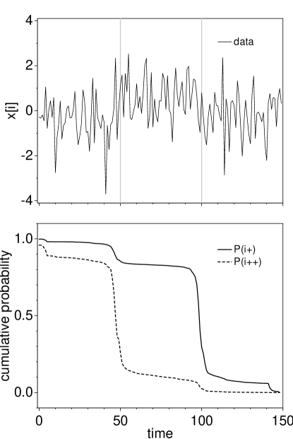
Figure 1: A time series with two changepoints (marked with gray lines), and estimated cumulative probabilities $P(i^{+})$ and $P(i^{++})$.

Figure 1 shows a time series with changepoints at $t=50$ and $t=100$. At the first changepoint, $\mu$ shifts from -0.5 to 0.5. At the second changepoint, it shifts to 0. Throughout, $\sigma$ is 1.0.

The bottom graph shows the cumulative sums of $P(i^{+})$ and $P(i^{++})$, estimated at $t=150$. Appropriately, $P(i^{+})$ shows a large mode near $t=100$, which actually is the most recent changepoint. There is a smaller mode near $t=50$, the location of the second-most-recent changepoint, and another near $t=142$, which is due to chance.

The estimated probabilities are not normalized, so they don’t always add up to one. In this case, the sum of $P(i^{++})$ for all $i$ is $0.96$, which indicates a 4% chance that we have not seen two changepoints yet.

3.6 Generalization to unknown $\mu_{0}$, $\sigma^{2}$

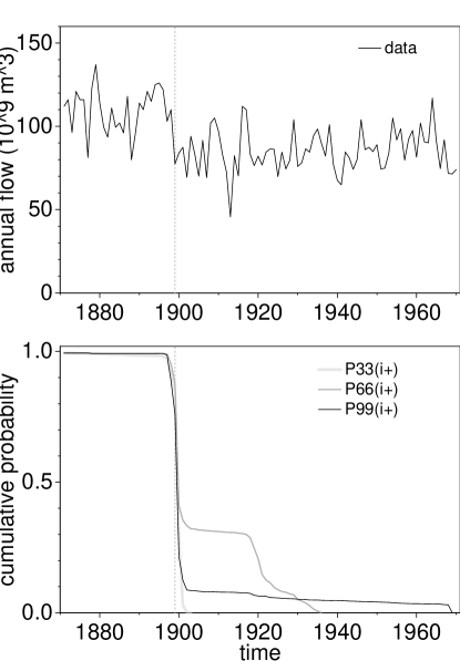
Figure 2: Average annual flow in the Nile river at Aswan from 1871 to 1970, and the estimated $P(i^{+})$ at $k=33,66,99$.

A feature of the proposed algorithm is that it extends easily to handle the cases when $\mu_{0}$ or $\sigma^{2}$, or both, are unknown. There are two possible approaches.

The simpler option is to estimate $\mu_{0}$ and/or $\sigma^{2}$ from the data and then plug the estimates into Equation 11. This approach works reasonably well, but because estimated parameters are taken as given, it tends to overestimate the probability of a changepoint.

An alternative is to use the observed $\bar{y}$ and $s^{2}$ to compute the posterior distributions for $\mu_{0}$ and/or $\sigma^{2}$ using Equations 8 and  10, and then make a random choice from those distributions (just as we did for $\mu_{1}$ in Section 3.1).

As an example, we apply our algorithm to the ubiquitous Nile data, a standard example in changepoint detection since Cobb’s seminal paper in 1978 [5]. This dataset records the average annual flow in the Nile river at Aswan from 1871 to 1970.

Figure 2 shows this data along with the estimated probability $P(i^{+})$ computed at three different times (after 33, 66 and 99 years). The salient feature at all three times is a high probability of a changepoint near 1898, which is consistent with the conclusion of other authors working with this data. At $k=66$, there is also a high probability of a changepoint near 1920, but by $k=99$ that hypothesis has all but vanished. Similarly, at $k=99$, there is a small probability that the last four data points, all on the low side, are evidence of a changepoint.

As time progresses, this algorithm is often quick to identify a changepoint, but also quick to “change its mind” if additional data fail to support the first impression. Part of the reason for this mercurial behavior is that $P(i^{+})$ is the probability of being the last changepoint; so a recent, uncertain changepoint might have a higher probability than a more certain changepoint in the past.

3.7 Detecting changes in variance

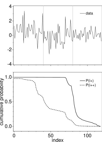
Figure 3: A time series with a change in mean and a change in variance.

To detect changes in variance, we can generalize the algorithm further by estimating $\sigma$ separately before and after the changepoint. In this case, the likelihood function is

$$P(X|i^{+})=\\ \prod_{j=1}^{i}P(x_{j}|\mu_{0},\sigma_{0}^{2})\prod_{j=i+1}^{n}P(x_{j}|\mu_{1},\sigma_{1}^{2})$$ (20)

where $\mu_{0}$ and $\sigma_{0}^{2}$ are drawn from the posterior distribution for the mean and variance before the changepoint, and likewise $\mu_{1}$ and $\sigma_{1}^{2}$ after the breakpoint.

Figure 3 shows a time series with a change in mean followed by a change in variance. Before the first changepoint, $\mu,\sigma=(1,1)$; after the first changepoint, $\mu,\sigma=(0,1)$; and after the second changepoint, $\mu,\sigma=(0,0.5)$.

Correctly, the estimated $P(i^{+})$ indicate a high probability near the last changepoint. The estimated $P(i^{++})$ indicate less certainty about the location of the second-to-last changepoint.

For this example the generalized algorithm works well, but its behavior is erratic when a series of similar values appear in the time series. In that case the estimated values of $\sigma_{1}^{2}$ tend to be small, so the computed probability of a changepoint is unreasonably high. We are considering ways to mitigate this effect without impairing the sensitivity of the algorithm too much.

4 Evaluation

The examples in the previous section show that the estimated values are reasonable, but not that they are accurate or more useful than results from other algorithms. Since there are no previous algorithms for computing $P(i^{+})$, there is no direct basis for comparison, but there are two evaluations we could perform:

• There are Bayesian methods that estimate $P(i)$; that is, the probability that there is a changepoint at any time $i$. From this we can compute $P(i^{+})$ and compare to our algorithm. We would like to pursue this approach in future work.

• Changepoint detection algorithms are often used “online” to raise an alarm when the evidence for a changepoint reaches a certain threshold. These algorithms are relatively simple to implement, and the criteria of merit are clear, so we start by evaluating our algorithm in this context.

The goal of online detection is to raise an alarm as quickly as possible after a changepoint has occurred while minimizing the frequency of false alarms.

Basseville and Nikiforov [1] propose a criterion for comparing algorithms in the case where an actual changepoint is equally likely to occur at any time, so the time of the first changepoint, $t_{0}$ is distributed geometrically.

During any given run, an algorithm has some probability of raising an alarm before $t_{0}$; this false alarm probability is denoted $\alpha$. Then, for a constant value of $\alpha$, the goal is to minimize the mean delay, $\tau=t_{a}-t_{0}+1$, where $t_{a}$ is the time of the alarm. In our experiements, we use a trimmed mean, for reasons explained below.

4.1 GLR

The gold standard algorithm for online changepoint detection is CUSUM (cumulative sum), which is optimal, in the sense of minimizing mean delay, when the parameters of the distribution are known before and after the changepoint [1].

When the parameters after the changepoint are not known, CUSUM can be generalized in several ways, including Weighted CUSUM and GLR (generalize likelihood ratio).

For the experiments in this section, we consider the case where the distribution of values before the changepoint is normal with known parameters $\mu_{0}$, $\sigma^{2}$; after the changepoint, the distribution is normal with unknown $\mu_{1}$ and the same known variance. We compare the performance of our algorithm to GLR, specifically using the decision function $g_{k}$ in Equation 2.4.40 from Basseville and Nikiforov [1].

The decision function $g_{k}$ is constructed so that its expected value is zero before the changepoint and increasing afterwards. When $g_{k}$ exceeds the threshold $h$, an alarm is raised, indicating that a changepoint has occurred (but not when). The threshold $h$ is a parameter of the algorithm that can be tuned to trade off between the probability of a false alarm and the mean delay.

4.2 CPP

It is straightforward to adapt our algorithm so that it is comparable with GLR. First, we adapt the likelihood function to use the known values of $\mu_{0}$ and $\sigma$, so only $\mu_{1}$ is unknown. Second, we use the decision function:

$$g_{k}=\sum_{i=0}^{k}P(i^{+})$$ (21)

This $g_{k}$ is the probability that a changepoint has occurred somewhere before time $k$. Our algorithm provides additional information about the location of the changepoint, but this reduction eliminates that information.

We call this adapted algorithm CPP, for “change point probability”, since the result is a probability (at least in the Bayesian sense) rather than a likelihood ratio.

Both GLR and CPP have one major parameter, $h$, which has a strong effect on performance, and a minor parameter that has little effect over a wide range. For GLR, the minor parameter is the minimum change size, $\nu_{min}$. For CPP, it is the prior probability of a changepoint, $f$.

4.3 Results

In our first experiment, $\mu_{0},\sigma=(0,1)$ and $\mu_{1}=1$, so the signal to noise ratio is $S/N=|\mu_{1}-\mu_{0}|/\sigma=1$. In the next section we will look at the effect of varying $S/N$.

In each trial, we choose the actual value of $t_{0}$ from a geometric distribution with parameter $\rho$, so

$$P(t_{0}=n)=(1-\rho)^{n-1}\rho$$ (22)

We set $\rho=0.02$, so the average value of $t_{0}$ is 50.

Each trial continues until an alarm is raised; the alarm time is denoted $t_{a}$. If $t_{a}\leq t_{0}$, it is considered a false alarm. Otherwise, we compute the delay time $t_{a}-t_{0}+1$.

To compute mean delay, we average over the trials that did not raise a false alarm. We use a trimmed mean (discarding the largest and smallest 5%) for several reasons: (1) the trimmed mean is generally more robust, since it is insensitive to a small numbers of outliers, (2) very short delay times are sometimes “right for the wrong reason”; that is, the algorithm was about to generate a false positive when the changepoint occurred, and (3) when $t_{0}$ is small, we see very few data points before the changepoint and $t_{a}$ can be arbitrarily large. In our trials, we quit when $k>t_{0}+100$ and set $t_{a}=\inf$. The trimmed mean allows us to generate a meaningful average, as long as fewer than 5% of the trials go “out of bounds”.

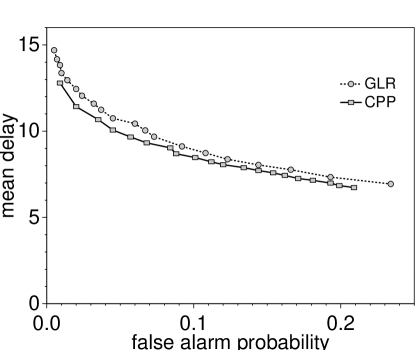
Figure 4: Mean delay versus false alarm probability for a range of threshold values.

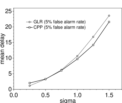
Figure 5: Mean delay versus $\sigma$ with false alarm probability $\alpha=0.05$.

The performance of both algorithms depends on the choice of the threshold. To compare algorithms, we plot mean delay versus false alarm probability for a range of thresholds. Then for a fixed false alarm probability, $\alpha$, we can see which algorithm yields a shorter mean delay.

Figure 4 shows the results averaged over 1000 runs. Both algorithms use the same random number generator, so they see the same data.

Across a wide range of $\alpha$, the mean alarm time for CPP is slightly better than for GLR; the difference is 0.5–1.0 time steps. For example, at $\alpha=0.05$, the mean alarm time is 9.7 for CPP and 10.7 for GLR (estimated by linear interpolation between data points).

This advantage increases as $\sigma$ increases (or equivalently as $S/N$ decreases). Figure 5 shows the mean alarm time with $\alpha=0.05$ for a range of values of $\sigma$. When $\sigma$ is small, the mean alarm time is small, and GLR has an advantage. But for $\sigma>0.7$ ($S/N<1.4$) CPP is consistently better.

We conclude that CPP is as good as GLR, or better, over a wide range of scenarios, and that the advantage increases as the signal-to-noise ratio decreases.

5 Conclusions

We have proposed a novel algorithm for estimating the location of the last changepoint in a time series that includes abrupt changes. The algorithm is Bayesian in the sense that the result is a joint posterior distribution of the parameters of the process, as opposed to a hypothesis test or an estimated value. Like other Bayesian methods, it requires subjective prior probabilities, but if we assume that changepoints are equally likely to occur at any time, the required prior is a single parameter, $f$, the probability of a changepoint.

This algorithm can be used for changepoint detection, location estimation, or tracking. In this paper, we apply it to the changepoint detection problem and compare it with a standard algorithm for this problem, GLR. We find that the performance is as good as GLR, or better, over a wide range of scenarios.

In this paper, we focus on problems where values between changepoints are known to be normally distributed. In some cases, data from other distributions can be transformed to normal. For example, several Internet characteristics are lognormal [12], which means that they are normal under a log transform. Alternatively, it is easy to extend our algorithm to handle any distribution whose pdf can be computed, but there is likely to be a performance penalty (the normal assumption is convenient in our implementation because its sufficient statistics can be updated incrementally with only a few operations).

We think that the proposed algorithm is promising, and makes a novel contribution to the statistics of changepoint detection. But this work is at an early stage; there is still a lot to do:

1. We have evaluated the proposed algorithm in the context of the changepoint detection problem, and demonstrated its use for estimating the location of a changepoint, but we have not evaluated its performance for location estimation and tracking. These problems take advantage of the full capability of the algorithm, so they will test it more rigorously.

2. In Section 3.7 we identified an intermittent problem when we use our algorithm to detect changes in variance. We are working on mitigating this problem.

3. A drawback of the proposed algorithm is that it requires time proportional to $n^{2}$ at each time step, where $n$ is the number of steps since the second-to-last changepoint. If the time between changepoints is more than a few thousand steps, it may be necessary to desample the data to control run time.

4. So far we have not addressed the autocorrelation structure that has been seen in many network measurements, but this work raises an intriguing possibility. If a time series actually contains abrupt changepoints, but no correlation structure between them, it will appear to have autocorrelation if we ignore the changepoints. In future work we plan to use changepoint detection to divide a time series of measurements into stationary intervals, and then investigate the autocorrelation structure within intervals to see whether it is possible that observed correlations are (at least in part) an artifact of stationary models.

References

- [1] M. Basseville and I. Nikiforov. Detection of abrupt changes: theory and application. Information and system science series. Prentice Hall, Englewood Cliffs, NJ., 1993., 1993.
- [2] P.K. Bhattacharya. Some aspects of change-point analysis. 23:28–56, 1994.
- [3] Rudolf B Blažek, Hongjoong Kim, Boris Rozovskii, and Alexander Tartakovsky. A novel approach to detection of denial-of-service attacks via adaptive sequential and batch-sequential change-point detection methods. In IEEE Systems, Man, and Cybernetics Information Assurance Workshop, 2001.
- [4] H. Chernoff and S. Zacks. Estimating the current mean of a normal distribution which is subject to changes in time. Annals of Mathematical Statistics, pages 999–1018, 1964.
- [5] G.W. Cobb. The problem of the Nile: Conditional solution to a changepoint problem. Biometrika, 65:243–252, 1978.
- [6] S. Deshpande, M. Thottan, and B. Sikdar. Early detection of BGP instabilities resulting from Internet worm attacks. In IEEE Global Telecommunications Conference, volume 4, pages 2266– 2270, 2004.
- [7] Andrew Gelman, John B. Carlin, Hal S. Stern, and Donald B. Rubin. Bayesian Data Analysis, Second Edition. Chapman & Hall/CRC, July 2003.
- [8] V. K. Jandhyala, S. B. Fotopoulos, and D. M. Hawkins. Detection and estimation of abrupt changes in the variability of a process. Comput. Stat. Data Anal., 40(1):1–19, 2002.
- [9] Thomas Karagiannis, Mart Molle, Michalis Faloutsos, and Andre Broido. A nonstationary Poisson view of Internet traffic. In INFOCOM, volume 3, pages 1558–1569, 2004.
- [10] Daniel Kifer, Shai Ben-David, and Johannes Gehrke. Detecting change in data streams. In Proceedings of the 30th International Conference on Very Large Data Bases, 2004.
- [11] Wael Noureddine and Fouad Tobagi. The Transmission Control Protocol. Technical report, Stanford University, July 2002.
- [12] Vern Paxson. Empirically derived analytic models of wide-area TCP connections. IEEE/ACM Transactions on Networks, 2(4):316–336, 1994.
- [13] M. H. Vellekoop and J. M. C. Clark. A nonlinear filtering approach to changepoint detection problems: Direct and differential-geometric methods. SIAM Review, 48(2):329–356, 2006.
- [14] Rich Wolski, Neil T. Spring, and Jim Hayes. The Network Weather Service: a distributed resource performance forecasting service for metacomputing. Future Generation Computer Systems, 15(5–6):757–768, 1999.
- [15] Y. Zhang, Nick Duffield, Vern Paxson, and Scott Shenker. On the constancy of Internet path properties. In ACM SIGCOMM, 2001.