Internal Extinction in the SDSS Late-Type Galaxies

Abstract

We study internal extinction of late-type galaxies in the Sloan Digital Sky Survey. We find that the degree of internal extinction depends on both the concentration index $c$ and $K_{s}$-band absolute magnitude $M_{K}$. We give simple fitting functions for internal extinction. In particular, we present analytic formulae giving the extinction-corrected magnitudes from the observed optical parameters. For example, the extinction-corrected $r$-band absolute magnitude can be obtained by $M_{r,0}=-20.77+(-1+\sqrt{1+4\Delta(M_{r,obs}+20.77+4.93\Delta)})/2\Delta$, where $\Delta=0.236\{1.35(c-2.48)^{2}-1.14\}\log(a/b)$, $c=R_{90}/R_{50}$ is the the concentration index, and $a/b$ is the isophotal axis ratio of the 25 mag/arcsec² isophote in the $i$-band. The $1\sigma$ error in $M_{r,0}$ is $0.21{\rm log}(a/b)$. The late-type galaxies with very different inclinations are found to trace almost the same sequence in the $(u-r)$-$M_{r}$ diagram when our prescriptions for extinction correction are applied. We also find that $(u-r)$ color can be a third independent parameter that determines the degree of internal extinction.

1. Introduction

Dust in spiral galaxies causes internal extinction. For example, due to dust, edge-on spiral galaxies in general look fainter than face-on spirals with the same intrinsic luminosity in short wavelength optical bands, in particular (see Fig. 12 of Choi, Park, & Vogeley 2007). The study of internal extinction is important for determination of distances and absolute magnitude of galaxies. Giovanelli et al. (1995) demonstrated that inadequate treatment of internal extinction has strong effects on the distances estimated using the Tully-Fisher relation (Tully & Fisher 1977). Internal extinction also causes biased measurements of galaxy star formation rates (see, for example, Bell & Kennicutt 2001; Sullivan et al. 2000) and affects determination of galaxy luminosity function (Shao et al. 2007). Earlier studies of internal extinction include Giovanelli et al. (1994, 1995), Tully et al. (1998), and Masters, Giovanelli, & Haynes (2003). Recent works that contain relevant discussions on the topic are Rocha et al. (2008), Unterborn & Ryden (2008), and Maller et al. (2008).

The amount of obscuration by dust is larger when the observing wavelength is shorter. Therefore, the effect of inclination is more pronounced in short-wavelength bands, such as $u$ or $r$ band, and it may be much smaller in $K_{s}$ (2.17$\mu$m) band. As a consequence, when the viewing angle changes for a given galaxy, $u$- or $r$-band magnitude changes while $K_{s}$-band magnitude does not change much. Therefore, $u-K_{s}$ or $r-K_{s}$ color tends to be larger when the galaxy is viewed more edge-on.

Internal extinction depends on many factors. Perhaps, the most important factor is the amount of dust. How dust is distributed can also be an important factor. The study of extinction versus inclination will ultimately reveal how dust is distributed and how much dust is contained in spiral galaxies. Then, what determines the amount and distribution of dust in spiral galaxies?

Earlier works have discussed dependence of internal extinction on luminosity. Giovanelli et al. (1995) found that the amount of internal extinction in $I$ band depends on the galaxy luminosity. Tully et al. (1998) also found a strong luminosity dependence using a magnitude-limited samples drawn from the Ursa Major and Pisces Clusters. Masters, Giovanelli, & Haynes (2003) studied internal extinction in spiral galaxies in the near infrared and also found a luminosity dependence. On the other hand, there are suggestions that internal extinction depends on galaxy type (de Vaucouleurs et al. 1991; Han 1992).

In this paper, we study the internal extinction in SDSS late-type galaxies. We investigate the dependence of the inclination effects on luminosity, concentration index $c$, and $u-r$ color. In §2, we describe the data set used in this paper. In §3, we study dependence of internal extinction on the concentration index $c$ and $K_{s}$-band luminosity separately. In §4, we measure dependence of internal extinction on the concentration index $c$ and $K_{s}$-band luminosity simultaneously. In §5, we derive dependence of inclination effects on $r$-band luminosity. The result in §5 is useful when $K$-band magnitude is not available. In §6, we present dependence on $u-r$ color. We give discussion in §7 and conclusion in §8.

2. Data and Method

In this study, we investigate how $u$- and $r$-band magnitudes behave as the inclination angle changes. The physical parameters we consider are $r$-band absolute magnitude $M_{r}$, $u-r$ color, the axis ratio $a/b$, and the concentration index $c$.

The primary data set we use is a subset of volume-limited SDSS (DR5) galaxy sample (the data set D1 in Choi et al. 2007). The redshift of the galaxies is between 0.0250 and 0.04374 and the minimum $r$-band absolute magnitude, $M_{r}$, is $-18.0+5{\rm log}h$, where $h$ is the Hubble constant divided by 100 km s^-1 Mpc^-1. In this paper, we assume the Hubble constant is 75km/sec/Mpc. Therefore, the absolute magnitude in this paper can be transformed to the $h$-dependent form by

$$M_{\lambda}^{h}=M_{\lambda}^{h=0.75}+5\log(h/0.75),$$ (1)

where $M_{\lambda}^{h=0.75}$ is the absolute magnitude we use in this paper. The rest-frame absolute magnitudes of galaxies are computed in fixed bandpasses, shifted to $z=0.1$, using Galactic reddening corrections (Schlegel, Finkbeiner, & Davis 1998) and $K$-corrections as described by Blanton et al. (2003). Therefore, all galaxies at $z=0.1$ have a $K$-correction of $-2.5{\rm log}(1+0.1)$, independent of their spectral energy distribution. We then apply the mean luminosity evolution correction given by Tegmark et al. (2004), $E(z)=1.6(z-0.1)$. The comoving distance limits of our volume-limited sample are 74.6 and 129.8 $h^{-1}$Mpc if we adopt a flat $\Lambda$CDM cosmology with density parameters $\Omega_{m}=0.27$ and $\Omega_{\Lambda}=0.73$. The galaxies in the volume-limited sample are divided into early (E and S0) and late (S and Irr) morphological types based on the location of galaxies in the $u-r$ color, $g-i$ color gradient, and concentration index space (Park & Choi 2005).

There are 14,032 late-type galaxies in the data set and, among them, $\sim$8,700 galaxies have matching data in the 2 Micron All-Sky Survey (2MASS) Extended Source Catalog. If the distance between the center of a SDSS galaxy and that of a 2MASS galaxy is less than the semimajor axis in the SDSS $i$-band, we consider they are identical. When there are multiple matches, we simply discard the data. We also remove data when the absolute value of the color gradient parameter ($\Delta(g-i)$; see Park & Choi 2005) is larger than 0.7, the $u-r$ color is larger that 4 or less than 0, or the H_α line width is less than 0 or larger than 200Å. About 700 galaxies have been discarded from this procedure.

2.1. Parameters

1) $M_{r}$, $M_{u}$, and $u-r$: We use $r$-band absolute Petrosian magnitudes and $u-r$ model color from the SDSS data. We obtain $u$-band absolute magnitude $M_{u}$ from the relation

$$M_{u}=M_{r}+(u-r).$$ (2)

Since the uncertainties in the extinction-corrections are large, we ignore the differences between the Petrosian $u$-band absolute magnitude and that derived from Equation (2).

2) $c$: The concentration index is defined by $R_{90}/R_{50}$ where $R_{50}$ and $R_{90}$ are the semimajor axis lengths of ellipses containing 50% and 90% of the Petrosian flux in the SDSS $i$-band image, respectively. It is corrected for the seeing effects by using the method described in Park & Choi (2005). It is basically a numerical inverse mapping from the image convolved with the PSF to the intrinsic image having a Sersic profile and a fixed inclination. The concentration index used here is the inverse of the one used by Park & Choi.

3) $a/b$: The isophotal axis ratio $a/b$ is from the SDSS $i$-band image. Here, $a$ is the major axis length and $b$ the minor axis length, corrected for the seeing effects. We choose the isophotal axis ratio because the isophotal position angles correspond most accurately to the true orientation of the major axis, which is true for barred galaxies in particular. Here we assume that outside the central region, the disk of a late-type galaxy can be approximated as a circular disk, which thus appears as an ellipse in projection. If the disk of late-type galaxies has an intrinsic non-circularity, our estimation of the $a/b$ ratio will have some error due to our assumption.

4) $M_{K}$: We use $K_{s}$-band magnitude (more precisely, magnitude within the 20th mag arcsec^-2 elliptical isophote set in $K_{s}$ band) from the 2 Micron All-Sky Survey (2MASS) data. We also apply $K$-corrections and Galactic extinction corrections for the 2MASS data as described by Masters, Giovanelli, & Haynes (2003). As in the SDSS case, the $K$-corrections are made for a fixed redshift of $z=0.1$. Most matched galaxies in our sample have $M_{K}$ brighter than $-20$.

Figure 1.— Distribution of the galaxies in our volume-limited sample in the $K_{s}$-band absolute magnitude $M_{K}$ and the concentration index $c=R_{90}/R_{50}$ space divided into $25\times 25$ cells.

2.2. Method

We adopt the popular parameterization of the effects of internal extinction:

$$A_{\lambda}=\gamma_{\lambda}\log_{10}(a/b),$$ (3)

where $A_{\lambda}$ is the amount of extinction. In this parameterization, $\gamma_{\lambda}$ is the slope of a scatter plot drawn on the $\log_{10}(a/b)$ - $A_{\lambda}$ plane. We will see in section 4 that this is actually a very reasonable model in the case of the SDSS galaxies even though some recent studies reported that better models can be found (Masters et al. 2003; Rocha et al. 2008; Unterborn & Ryden 2008).

Our goal is to find the values of $\gamma_{r}$ and $\gamma_{u}$. To find $\gamma_{r}$ (or $\gamma_{u}$), we first plot $r-K_{s}$ (or $u-K_{s}$) against $\log_{10}(a/b)$. Then, the slopes of the scatter plot are

$$\gamma_{r-K} \approx \gamma_{r}-\gamma_{K},\mbox{~{}~{}~{}~{}~{} and}$$

$$\gamma_{u-K} \approx \gamma_{u}-\gamma_{K}.$$ (4)

When no strong extinction is present in $K_{s}$ band, we can write

$$\gamma_{r-K} \approx \gamma_{r},\mbox{~{}~{}~{}~{}~{} and}$$

$$\gamma_{u-K} \approx \gamma_{u}.$$ (5)

In this paper, we assume that $K_{s}$-band magnitude is almost free of inclination effects. Masters et al. (2003) analyzed galaxies in the 2MASS Extended Source Catalog and concluded that the internal extinction is indeed small in $K_{s}$ band. Their results are consistent with the earlier result that $\gamma_{K}\sim 0.22$ (Tully et al. 1998).

Figure 2.— Dependence of colors on the concentration index $c$ ($\equiv R_{90}/R_{50}$). When $c$ is small, the colors only weakly depend on the axial ratio $a/b$. The axial ratio is derived from the SDSS $i$-band image.

Figure 3.— Dependence of the slope of the extinction law on $c$ ($\equiv R_{90}/R_{50}$). Solid lines are the slopes of the linear fit to the most probable values in $\log(a/b)$ bins between $\log(a/b)=0$ and 0.5. Dotted lines are the slopes of the linear fit to the median. (Left panel) $\gamma_{r-K}$. (Middle panel) $\gamma_{u-K}$. (Right panel) $\gamma_{u-r}$.

As shown by earlier studies, $\gamma_{\lambda}$ depends on luminosity (Giovanelli et al. 1995; Tully et al. 1998) and/or galaxy type (de Vaucouleurs et al. 1991; Han 1992). In this study, our primary concern is the dependence of $\gamma_{\lambda}$ on $K_{s}$-band luminosity and the concentration index $c$. In Figure 1, we plot the galaxies on the $c-M_{K}$ plane. On the plot, we show $25\times 25$ cells. The coordinates of the cell centers, $(c_{m},K_{n})$, are given by

$$c_{m} = 1.68+0.06m,\mbox{~{}~{}~{}m= 0, 1,..., 24,~{}~{}~{} and}$$ (6)

$$K_{n} = -23.4+0.15n,\mbox{~{}~{}~{}n= 0, 1,..., 24.}$$ (7)

Note that $c_{2}=1.8$, $c_{22}=3.0$, $K_{2}=-23.1$, and $K_{22}=-20.1$.

When we investigate the dependence of $\gamma_{\lambda}$ on $M_{K}$ and $c$, we may simply use galaxies in each cell in Figure 1. However, some cells in Figure 1 are not sufficiently populated. Therefore, for smooth results, we use galaxies in $5\times 5$ cells for scatter plots. More precisely, we use galaxies with $c_{m}-2.5(\Delta c)\leq c\leq c_{m}+2.5(\Delta c)$ and $K_{n}-2.5(\Delta K)\leq M_{K}\leq K_{n}+2.5(\Delta K)$, where $\Delta c=0.06$ and $\Delta K=0.15$. We allow for a similar overlap when we study $M_{K}$- or $c$-dependence separately.

To find the slopes, we divide $\log(a/b)$ axis into 20 bins between 0 and 1. Then we find a representative value for each bin. We try two methods to obtain the representative value:

$$\begin{array}[]{l}\mbox{1) the median}\\ \mbox{2) the most probable value.}\end{array}$$

To fine the most probable value in each $\log(a/b)$ bin, we use a smoothing function

$$\phi(x,y)=\left\{\begin{array}[]{ll}\exp{(-(y-y_{i})^{2}/2\sigma_{y}^{2})}&\mbox{ if $|x-x_{i}|$ $\leq$ 0.05}\\ 0&\mbox{ otherwise,}\end{array}\right.$$ (10)

where $x=\log_{10}(a/b)$, $x_{i}$ ($y_{i}$) is the $x$ ($y$) value of the $i^{th}$ galaxy, and $\sigma_{y}$ is the standard deviation. After applying the smoothing function, we find the maximum value of the smoothed distribution in each bin. After finding representative values in bins of $\log(a/b)$, we perform the linear fit to the representative values between $\log(a/b)=0$ and 0.5.

Figure 4.— Dependence of colors on $M_{K}$. Faint galaxies in $K_{s}$ band exhibit shallower slopes in all 3 colors, while bright galaxies show steep slopes.

Figure 5.— Dependence of the slope of the extinction law on the $K_{s}$-band absolute magnitude $M_{K}$. Solid lines are the slopes of the linear fit to the most probable values in $\log(a/b)$ bins between $\log(a/b)=0$ and 0.5. Dotted lines are the slopes of the linear fit to the median. (Left panel) $\gamma_{r-K}$. (Middle panel) $\gamma_{u-K}$. (Right panel) $\gamma_{u-r}$.

3. Dependence on $c$ or $M_{K}$

3.1. Dependence on $c$

In this subsection, we consider only $c$-dependence. We plot $r-K_{s}$, $u-K_{s}$, and $u-r$ colors against $\log_{10}(a/b)$ in Figure 2. As we mentioned earlier, when we draw the scatter plot for $c=c_{m}$, we use galaxies with $c_{m}-2.5(\Delta c)\leq c\leq c_{m}+2.5(\Delta c)$, where $\Delta c=0.06$. Therefore, the plot for $c=1.80$ contains galaxies with $1.65\leq c\leq 1.95$, for example.

We can see that the slope, hence $\gamma_{\lambda}$, for $c=1.80$ is smaller than those for other $c$ values. Note that the slope for $c=1.80$ is very close to zero for $u-r$ color.

Figure 3 shows dependence of the slope on $c$. All 3 colors show a common feature: the slope peaks near $c\sim 2.5$. This means that internal extinction is maximum for intermediate late-type galaxies, and is smaller for early and late late-type galaxies. On the other hand, $u-r$ and $u-K_{s}$ show stronger dependence on $c$ than $r-K_{s}$, telling that internal extinction is higher in shorter wavelength bands. The quadratic equations on the plots are the fitting functions. The solid curves are for the most probable values and the dotted curves for the median. The RMS scatters of the measured slope from the fitting functions (for the most probable values) are 0.071, 0.170, and 0.154 for $r-K_{s},u-K_{s}$, and $u-r$ colors, respectively. We list the quadratic fits, $\gamma(c)$’s, in Table 1 and 2.

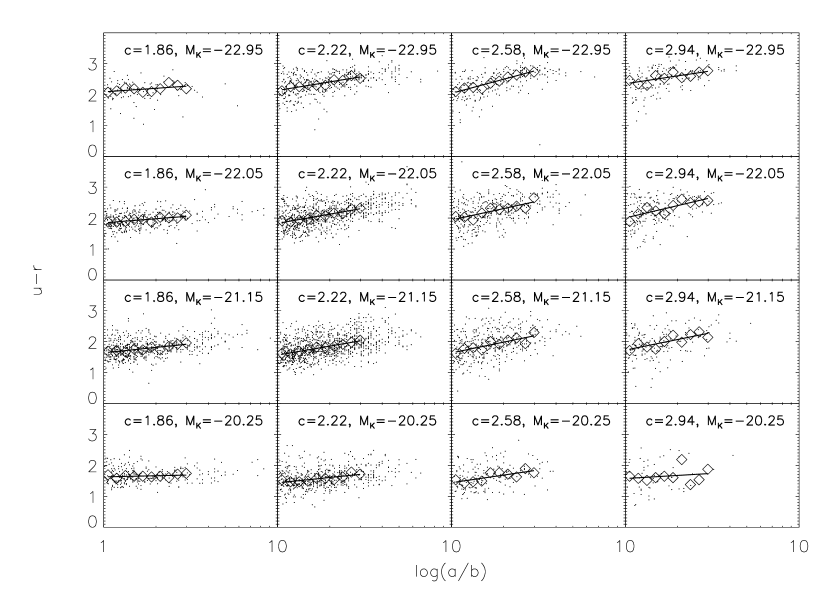
Figure 6.— Scatter plots for $u-r$. Diamonds denote the most probable values in $\log(a/b)$ bins. Lines are the results of the least square fit to the diamonds. Only points with $\log_{10}(a/b)\leq 0.5$ are used for fitting.

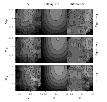
Figure 7.— The measured slopes of the extinction law (left panels), fitting functions (middle panels), and the difference between the measured slopes and the fitting functions (right panels). (Upper panels) $r$-$K_{s}$ color. (Middle panels) $u$-$K_{s}$ color. (Lower panels) $u-r$ color. The horizontal axis of each contour plot is the concentration index $c$ ($\equiv R_{90}/R_{50}$) and the vertical axis is the $K_{s}$-band absolute magnitude $M_{K}$. The contours are drawn at intervals of 0.2 (upper panels), 0.4 (middle panels), and 0.2 (lower panels), respectively.

3.2. Dependence on $M_{K}$

In this subsection, we consider $M_{K}$-dependence of internal extinction. We plot $r-K_{s}$, $u-K_{s}$, and $u-r$ colors against $\log_{10}(a/b)$ in Figure 4. When we draw the scatter plot for $M_{K}=K_{n}$, we use galaxies with $K_{n}-2.5(\Delta K)\leq M_{K}\leq K_{n}+2.5(\Delta K)$, where $\Delta K=0.15$. For example, the plot for $M_{K}=-23.1$ contains galaxies with $-23.475\leq M_{K}\leq-22.725$.

We can clearly see that the slope, hence $\gamma_{\lambda}$, for $M_{K}=-20.1$ is smaller than those for other $M_{K}$ values. Note that the slope for $M_{K}=-20.1$ is very close to zero for all 3 colors.

Figure 5 shows dependence of the slope on $M_{K}$. All 3 colors have a common feature: the slope is higher when galaxies are brighter in $K_{s}$ band. Due to lack of data points, the slope is not clear for $M_{K}\lesssim-23.2$. Therefore, one should be careful when using the fitting functions shown on the plots for galaxies with $M_{K}\lesssim-23.2$. The RMS scatters of the measured slope from the fitting functions (for the most probable values) are 0.071, 0.110, and 0.075 for $r-K_{s},u-K_{s}$, and $u-r$ colors, respectively. We list the quadratic fits, $\gamma(M_{K})$’s, in Table 1 and 2.

4. Dependence on $c$ and $M_{K}$

We now study dependence of $r-K_{s},u-K_{s},$ and $u-r$ colors on the concentration index and $K_{s}$-band absolute magnitude. In Figure 6 we plot $u-r$ against $\log_{10}(a/b)$ as a function of $c$ and $M_{K}$. The diamonds are the most probable values in bins of $\log(a/b)$. The lines are the least square fits to the most probable values. It can be seen that the reddening is fit well by our extinction model linear in ${\rm log}_{10}(a/b)$ (i.e. Equ. 3), and that the slope depends on both $c$ and $M_{K}$. Plots for $r-K_{s}$ and $u-K_{s}$ show behaviors similar to the $u-r$ case. We also obtained the fits to the median, which are qualitatively similar to the most probable case.

In the top panels of Figure 7 we present contour plots of the measured slopes of $r-K_{s}$ color, $\gamma_{r-K}$. The upper-left panel is for $\gamma_{r-K}$ based on the most probable values. The function

$$\gamma_{r-K}(c,M_{K})=1.02\gamma_{r-K}(c)\gamma_{r-K}(M_{K}),$$ (11)

shown in the upper-middle panel, fits well the slopes based on the most probable values (see Table 1). Since we do not have enough bright galaxies in $K_{s}$ band, we do not have a reliable fitting formula for $M_{K}<-23.25$. Although our fitting formula suggests that the slope declines when $M_{K}$ becomes less than $\sim-22.9$, the true behavior of the slope may be different. Therefore, instead of using the fitting formula in Equation (11), one may use

$$\gamma_{r-K}(c,M_{K})=1.02\times 1.14\gamma_{r-K}(c)$$ (12)

for $M_{K}<-22.9$. The upper-right panel of Figure 7 shows the difference between the measured slope and the fitting function. The RMS value of the difference is 0.174 while the peak slope is about 1.4. See Table 2 for a fitting function based on the median.

Similarly, we present contours of $\gamma_{u-K}$ and $\gamma_{u-r}$ in the middle and bottom panels of Figure 7, respectively. The fitting functions for the most probable values are

$$\gamma_{u-K}(c,M_{K})=0.48\gamma_{u-K}(c)\gamma_{u-K}(M_{K}),$$ (13)

$$\gamma_{u-r}(c,M_{K})=0.94\gamma_{u-r}(c)\gamma_{u-r}(M_{K})$$ (14)

(see Table 1). Again the fitting functions are uncertain for $M_{K}\lesssim-23.2$. The RMS differences, shown in the middle-right and lower-right panels of Figures 7, are 0.354 and 0.234, respectively. See Table 2 for fitting functions based on the median.

Figure 8.— Dependence of colors on the intrinsic (i.e. face-on) $r$-band absolute magnitude $M_{r,0}$. We use $\gamma_{R}\sim\gamma_{r-K}\sim\gamma_{r-K}(c,M_{k})$ (see Table 1) to derive $M_{r,0}$. When $M_{r,0}\lesssim-19$, internal extinction is very small.

Figure 9.— Dependence of $\gamma$ on the intrinsic (i.e. face-on) $r$-band absolute magnitude $M_{r,0}$. Solid lines are the slopes of the linear fit to the most probable values in $\log(a/b)$ bins between $\log(a/b)=0$ and 0.5. Dotted lines are the slopes of the linear fit to the median. The RMS scatters of the measured slope from the fitting functions (for the most probable values) are 0.064, 0.095, and 0.070 for $r-K_{s},u-K_{s}$, and $u-r$ colors, respectively. (Left panel) $\gamma_{r-K}$. (Middle panel) $\gamma_{u-K}$. (Right panel) $\gamma_{u-r}$.

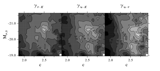
Figure 10.— Dependence of the slope of the extinction law for the $r-K$, $u-K$, and $u-r$ colors on the $r$-band absolute magnitude $M_{r,0}$ and the concentration $c$. The slope $\gamma$ is based on the most probable values. X-axis is the concentration index ($=R_{90}/R_{50}$). The contour intervals for $r$-$K_{s}$, $u$-$K_{s}$, and $u-r$ are 0.2, 0.4, and 0.2, respectively.

5. Dependence on r magnitude

When $K_{s}$-magnitude is not available, we cannot use the fitting functions derived in the previous section. In this section we present a method that utilizes $r$-magnitude, instead of $K_{s}$-magnitude. We consider $\gamma$’s derived from the most probable values.

5.1. Dependence on $M_{r,0}$

We obtain intrinsic (or face-on) $r$-band absolute magnitude, $M_{r,0}$, from

$$M_{r,0}=M_{r,obs}-\gamma_{R}(c,M_{K})\log_{10}(a/b),$$ (15)

where $M_{r,obs}$ is the $r$-band absolute magnitude before inclination corrections and $\gamma_{r}(c,M_{K})\sim\gamma_{r-K}(c,M_{K})$ is given in Table 1. Note that $\gamma_{r-K}(c,M_{K})\geq 0$. The RMS differences between the measured slopes and the fitting functions given in the last column of Table 1, are 0.208, 0.390, and 0.233 for $r-K_{s},u-K_{s}$, and $u-r$ colors, respectively. After obtaining $M_{r,0}$ we investigate how internal extinction depends on the intrinsic $r$-band luminosity.

Scatter plots in Figure 8 clearly shows that the slopes of the extinction in $r-K_{s},u-K_{s}$, and $u-r$ colors depend on the $r$-band absolute magnitude $M_{r,0}$. The slopes of the scatter plots are very small when $M_{r,0}=-18.80$, which means there is very little extinction in galaxies much fainter than the $M_{*}$ galaxies. (But note that late-type galaxies tend to be irregulars at fainter magnitudes and that irregulars have patchy distribution of dust which can cause a weaker dependence of extinction on inclination.)

Figure 10 show the behavior of the slopes on $c-M_{r,0}$ plane. It is interesting that there is a well-defined peak near $(c,M_{r,0})\sim(2.5,-20.8)$. In the $r$-band, the internal extinction is maximum at the absolute magnitude very close to the characteristic magnitude $M_{*}$ (see Table 2 of Choi et al. (2007) for $M_{*}$ measurements for the late-type SDSS galaxies. Note that $h=0.75$ is used in the present work.) The contour spacing for $\gamma_{r-K}$ (left panel) is 0.2 and the value of $\gamma_{r-K}$ at the center of the peak is greater than $\sim 1.6$. We can also see a similar peak for $\gamma_{u-K}$ (middle panel). However, the location of the peak for $\gamma_{u-r}$ (right panel) is somewhat different.

Figure 9 shows the dependence of the slope on $M_{r,0}$. The fitting functions are also shown on the plots.

Figure 11.— Comparisons between the inclination correction method using $\gamma(c,M_{K})$ and $\gamma$’s in the shorter bands. The inclination correction using $\gamma(c,M_{K})$ is straight forward. However, the use of $\gamma(c,M_{r,0})$ requires one more step (see Eq. 20) to get $M_{r,0}$ first.

5.2. Obtaining $M_{r,0}$ from $M_{r,obs}$ and $c$

We cannot observe the intrinsic $r$-band absolute magnitude $M_{r,0}$ directly. But we can obtain $M_{r,0}$ by solving the following equation:

$$M_{r,0}+\gamma_{r-K}(c,M_{r,0})\log_{10}(a/b)=M_{r,obs},$$ (16)

where $M_{r,obs}$, $c$, and $a/b$ are observed quantities. When we use a quadratic approximation as shown in Figure 9, then Eq. 16 becomes

$$M_{r,0}+\Delta[(M_{r,0}+20.77)^{2}-1.10/0.223]=M_{r,obs},$$ (17)

where

$$\Delta\equiv 1.06\times 0.223\times[1.35(c-2.48)^{2}-1.14]\log_{10}(a/b)\leq 0.$$ (18)

Equivalently, we have

$$(M_{r,0}+20.77)+\Delta[(M_{r,0}+20.77)^{2}-4.93]=(M_{r,obs}+20.77).$$ (19)

The solution is

$$M_{r,0}=-20.77+\frac{-1+\sqrt{1+4\Delta(M_{r,obs}+20.77+4.93\Delta)}}{2\Delta},$$ (20)

which gives the correct answer when $\Delta$ goes to zero. This equation is valid for $[(M_{r,0}+20.77)^{2}-4.93]<0$ and $\Delta<0$. When $[(M_{r,0}+20.77)^{2}-4.93]\geq 0$ or $\Delta\geq 0$, we simply have $M_{r,0}=M_{r,obs}$.

Figure 11 shows that extinction corrections using $M_{r}$ and $c$ give results quite close to those using $M_{K}$ and $c$. In the left panel, we obtain the intrinsic r-band absolute magnitude using two methods. For the x-axis, we make inclination corrections using

$$\gamma_{r}\sim\gamma_{r-K}=\gamma_{r-K}(c,M_{K}),$$ (21)

where $\gamma_{r-K}(c,M_{K})$ is given in Table 1. For y-axis, we make inclination corrections using Eq. (20). The left panel shows that the two methods give a good agreement. The middle and right panels are obtained similarly. The $1\sigma$ error in $M_{r,0}$ derived from $M_{r,obs}$ and $c$ is given by the error in $\gamma_{r-K}$(c,$M_{r,0}$) times ${\rm log}(a/b)$ (see Eq. 14) or $0.208{\rm log}(a/b)$ over the range from $M_{r,0}=-18.5$ to $-22.5$.

5.3. Obtaining $M_{u,0}$ and $(u-r)_{0}$

We can estimate $M_{u,0}$ from $M_{r,obs}$ and $c$. First, we need to obtain $M_{u,0}$ as described in the previous subsection. $M_{u,0}$ is

$$M_{u,0}=M_{u,obs}-\gamma_{u-K}(c,M_{r,0})\log_{10}(a/b),$$ (22)

where $\gamma_{u-K}(c,M_{r,0})$ is given in Table 1.

We can also estimate $(u-r)_{0}$ from $a/b$ and $c$. First, we need to obtain $M_{r,0}$. Then, $(u-r)_{0}$ is

$$(u-r)_{0}=(u-r)_{a/b}-\gamma_{u-r}(c,M_{r,0})\log_{10}(a/b),$$ (23)

where $\gamma_{u-r}(c,M_{r,0})$ is given in Table 1.

6. Dependence on $u-r$ color

In this paper, we have mainly considered dependence of $\gamma_{\lambda}$ on $K$ and $c$. There may be more parameters that determine $\gamma_{\lambda}$. In this section, we show that $u-r$ color can be a third independent parameter.

6.1. Slope vs. $(u-r)_{0}$

We obtain the intrinsic color, $(u-r)_{0}$, as follows:

$$(u-r)_{0}=(u-r)_{a/b}-\gamma_{u-r}(c,M_{r,0})\log_{10}(a/b),$$ (24)

or,

$$(u-r)_{0}=(u-r)_{a/b}-\gamma_{u-r}(c,M_{K})\log_{10}(a/b),$$ (25)

where $\gamma_{u-r}(c,M_{r,0})$ and $\gamma_{u-r}(c,M_{K})$ are given in Table 1. In this section, we use Eq. (25).

Figure 12 shows that $\gamma_{r-K}$ strongly depends on $(u-r)_{0}$. The Figure shows that the slope for $r-K_{s}$ is virtually zero when $(u-r)_{0}$ is less than $\sim 1.0$. The slope increases as the color increases. It seems that the slope reaches a maximum at $(u-r)_{0}\sim 2.5$. The behavior of the slope is uncertain for $(u-r)_{0}\gtrsim 2.5$.

Figure 12.— Dependence of $\gamma_{r-K}$ on $(u-r)_{0}$, where the subscript ’$0$’ denotes the inclination corrected value. We use $\gamma_{u-r}=\gamma_{u-r}(c,M_{K})$ (see Table 1) to derive the intrinsic color.

Figure 13.— $(u-r)_{0}$ as a third parameter. This figure shows that the slope depends not only on $c$ and luminosity but also the intrinsic $(u-r)$ color. Internal extinction is more significant when galaxies have larger intrinsic $(u-r)$ color.

6.2. Dependence of $(u-r)_{0}$ on $c$ or $M_{K}$

In this section, we investigate the possibility of $(u-r)_{0}$ as a third parameter. The third parameter should be independent of the first 2 parameters (i.e. $c$ and $M_{K}$ in our case). However, Figure 6 shows that $(u-r)_{0}$, which corresponds to the y intercepts of the linear fits, depends on the both $c$ and $M_{K}$. Therefore, $(u-r)_{0}$ is not a completely independent parameter, which means we cannot tell whether the change in slope observed in Figure 12 is entirely due to $(u-r)_{0}$ or just a different realization of $c$ or $M_{K}$ dependency through the correlation between them and $(u-r)_{0}$.

However, a careful look at Figure 6 reveals that $(u-r)_{0}$ varies between $\sim 1.5$ and $\sim 2.0$. One exception is the $(u-r)_{0}$ (i.e. the y intercept) in the upper-right panel, which is as large as $\sim 2.4$. From this observation, we can conclude that the intrinsic scatter in $(u-r)_{0}$ itself is larger than the systematic change in $(u-r)_{0}$ due to $c$ or $M_{K}$ change. Therefore, if we properly limit the ranges of $c$ and $M_{K}$ and draw a plot similar to Figure 12, then we can tell whether or not $\gamma_{r-K}$ really depends on $(u-r)_{0}$.

For this purpose, we only consider galaxies in the following ranges:

$$\begin{array}[]{l}\mbox{group 1: $-22.0\leq M_{K}\leq-21.4$ and $1.8\leq c\leq 2.1$}\\ \mbox{group 2: $-22.0\leq M_{K}\leq-21.4$ and $2.1\leq c\leq 2.4$}\\ \mbox{group 3: $-21.4\leq M_{K}\leq-20.8$ and $1.8\leq c\leq 2.1$}\\ \mbox{group 4: $-21.4\leq M_{K}\leq-20.8$ and $2.1\leq c\leq 2.4$}\\ \end{array}$$

Then, we study the dependence of $\gamma_{r-K}$ on $(u-r)_{0}$ for each group.

6.3. $(u-r)_{0}$ color as a third parameter

The discussion above indicates that the systematic change in $(u-r)_{0}$ in each group due to changes in $c$ and $M_{K}$ should be marginal. Figure 13 shows the possibility that $(u-r)_{0}$ can be a 3rd parameter: For given $c$ and $M_{K}$, the slope $\gamma_{\lambda}$ shows dependence on $(u-r)_{0}$. The general trend is that the slope is steeper, when $(u-r)_{0}$ is larger. Note, however, that galaxies in group 4 do not show strong dependence on $(u-r)_{0}$, while those in group 3 show a very strong dependence.

Figure 14.— Distributions of late-type galaxies in the color magnitude diagram. Galaxies with $a/b\leq$ 1.25 ($b/a\geq$ 0.8) are shown in the left panel, and those with $a/b\geq$ 2.5 ($b/a\leq$ 0.4) are shown in the middle panel. Distribution of all galaxies after inclination corrections are drawn on the right panel. The median color-magnitude relations are also drawn. We find that the group of highly inclined galaxies is significantly shifted with respect to the almost face-on ones toward fainter magnitudes and redder colors.

7. Discussion

Qualitatively speaking, our results are consistent with earlier claims that the extinction in spirals depends on luminosity (Giovanelli et al. 1995; Tully et al. 1998). Tully et al. (1998) derived an extinction law in $R$ band. They found that galaxies with $M_{R}$ reaching $-21$ mag have $\gamma_{R}\sim 1.16$ and the amplitude of extinction drops rapidly as luminosity decreases. Similarly, our Figure 9 shows that $\gamma_{r-K}\sim 1.1$ for $M_{r}\sim-21$ and it declines rapidly with decreasing luminosity. However, there are also differences. For example, $\gamma_{R}$ in Tully et al. (1998) reaches as large as $\sim 1.4$ for galaxies brighter than -21 mag in the $R$ band. We do not observe such a rise of $\gamma_{r}$ in our results. However, since the definition of $r$-magnitude is different and $\gamma_{r}$ depends on other parameters, such as $c$ and $u-r$, it is very difficult to understand the origin of this discrepancy.

Shao et al. (2007) found $\gamma_{r}\sim 1.37$ when they used the $r$-band axis ratio, which is substantially larger than our values. The difference may stem from the difference in fitting methods. We studied how $r-K_{s}$ color changes as a/b changes. Therefore the value of $\gamma$ in our study is actually $\gamma_{r-K}$, not $\gamma_{r}$. The value of $\gamma_{r}$ will be given by $\gamma_{r}\sim\gamma_{r-K}+\gamma_{K}\sim 1.15+0.26\sim 1.41$, where $1.15$ is the average value of $\gamma_{r-K}$ near the maximum (see Figure 5) and $0.26$ is the estimated $\gamma_{k}$ (Masters et al. 2003). The definition of $a/b$ is also different. Our $a/b$ is the $i$-band isophotal axis ratio, while that of Shao et al. (2007) is the $r$-band axis ratio obtained from the best fit of the images of galaxies with an exponential profile convolved with the point spread function.

On the other hand, there are several observations in $I$ band. Giovanelli et al. (1994) found the extinction in $I$ band of $\gamma_{I}\sim 1.05\pm 0.08$. Masters et al. (2003) found that $\gamma_{I}\sim 0.94$. Therefore, our result of $\gamma_{r}\sim 1.1$ agrees with the common wisdom: there is more extinction in shorter passband.

The concentration index, $c$, is related to morphology of late-type galaxies. Earlier studies show that, on average, early late-type galaxies have higher concentration (see, for example, Shimasaku et al. 2001; Strateva et al. 2001; Goto et al. 2003; Yamauchi et al. 2005). Therefore dependence of inclination effects on the concentration index implies that galaxy morphology is an important factor, which is consistent with earlier findings (see, for example, de Vaucouleurs et al. 1991; Han 1992). It is interesting that internal extinction is maximum when $c\sim 2.5$ which corresponds to Sb galaxies (see Shimasaku et al. 2001).

Choi et al. (2007) have shown that the sequence of late-type galaxies in the color-magnitude diagram can be significantly affected by the internal extinction. When the sequences are compared between late types with $b/a>0.8$ (nearly face-on) and $b/a<0.4$ (nearly edge-on), a very large departure is observed for the sequence of the inclined late-type galaxies relative to that of the face-on late types as the inclined galaxies appear fainter and redder. The degree of departure was found to be maximum for intermediate luminosity late types with $M_{r}\approx-20.5+5{\rm log}h=-21.1$. No such extinction effect was found for early-type galaxies. It will be very interesting to see if our extinction-correction prescription restores the color-magnitude diagram of inclined late-type galaxies.

In Figure 14, we plot our late-type galaxies in the color magnitude diagram. The left panel of Figure 14 shows the galaxies with $a/b\leq$ 1.25 ($b/a\geq$ 0.8) and the middle shows those with $a/b\geq$ 2.5 ($b/a\leq$ 0.4). We find that the group of highly inclined galaxies is significantly shifted with respect to the almost face-on ones toward fainter magnitude and redder colors. The result in Figure 12 indicates that the color of very blue galaxies is less affected by the internal extinction. However, Figure 12 does not tell much about color change of very red galaxies (i.e. redder than $u-r\sim$ 2.5) due to lack of data. Note that Choi et al. (2007) observed that both very blue and very red galaxies are less effected by the internal extinction. The right panel of Figure 14 is the inclination-corrected color magnitude diagram. The inclination correction is done based on $M_{K}$- and $c$-dependence of $M_{r}$ and $u-r$. To be more specific, we use Eqs. (13) and (21) to obtain $M_{r,0}$ and $(u-r)_{0}$. We do not draw the reddening vectors (caused by internal extinction) on the color-magnitude diagram becase, due to $c$-dependency, infinite number of reddening vectors are possible for a given value of ($M_{r}$, $u-r$). If one wish to draw ‘average’ reddening vectors for a fixed value of $\log(a/b)$, one can do that by using $\gamma_{u-r}(M_{r,0})$ and $\gamma_{r}(M_{r,0})$ in Table 1 (or 2). Of course, to get the $\gamma$ values, we first need to obtain $M_{r,0}$ from Eq. (20).

8. Conclusion

Our major conclusions are as follows.

1. We have shown that the slope $\gamma_{\lambda}$ depends on both $K_{s}$-band absolute magnitude $M_{K}$ and the concentration index $c$. The fitting functions for the relations are given in Table 1 and 2.

2. We have also shown that the slope $\gamma_{\lambda}$ depends on both the concentration index $c$ and $r$-band absolute magnitude $M_{r,0}$, where the subscript ‘$0$’ denotes the value after inclination correction. The relations are also given in Table 1 and 2.

3. We have derived analytic formulae giving the extinction-corrected magnitudes from the observed optical parameters (see, for example, Equation (20)).

4. We have shown that $(u-r)_{0}$ can be a third parameter that determines the slope $\gamma_{\lambda}$.

Table 1Fitting Functions (for most probable values)

	Dependence on c	Dependence on $M_{K}$	Dependence on $M_{r,0}$	$M_{K}$ & c	$M_{r,0}$ & c
	$\gamma(c)$	$\gamma$($M_{K}$)	$\gamma$($M_{r,0}$)	$\gamma$(c,$M_{K}$)	$\gamma$(c,$M_{r,0}$)
$r$-$K_{s}$	-1.35(c-2.48)2+1.14	-0.089($M_{K}$+22.9)2+1.16	-0.223($M_{r,0}$+20.8)2+1.10	1.02$\gamma(M_{K})\gamma(c)$	1.06$\gamma(M_{r,0})\gamma(c)$
$u$-$K_{s}$	-3.37(c-2.57)2+2.61	-0.187($M_{K}$+22.9)2+2.24	-0.318($M_{r,0}$+20.8)2+2.04	0.48$\gamma(M_{K})\gamma(c)$	0.52$\gamma(M_{r,0})\gamma(c)$
$u-r$	-2.02(c-2.63)2+1.49	-0.098($M_{K}$+22.9)2+1.09	-0.095(Mr,0+20.9)2+0.94	0.94$\gamma(M_{K})\gamma(c)$	1.03$\gamma(M_{r,0})\gamma(c)$

Table 2Fitting Functions (for the median)

	Dependence on c	Dependence on $M_{K}$	Dependence on $M_{r,0}$	$M_{K}$ & c	$M_{r,0}$ & c
	$\gamma(c)$	$\gamma$($M_{K}$)	$\gamma$($M_{r,0}$)	$\gamma$(c,$M_{K}$)	$\gamma$(c,$M_{r,0}$)
$r$-$K_{s}$	-1.13(c-2.49)2+1.08	-0.072($M_{K}$+23.1)2+1.13	-0.215($M_{r,0}$+20.8)2+1.08	1.07$\gamma(M_{K})\gamma(c)$	1.09$\gamma(M_{r,0})\gamma(c)$
$u$-$K_{s}$	-2.84(c-2.61)2+2.49	-0.154($M_{K}$+23.1)2+2.21	-0.296($M_{r,0}$+20.9)2+1.99	0.52$\gamma(M_{K})\gamma(c)$	0.55$\gamma(M_{r,0})\gamma(c)$
$u-r$	-1.70(c-2.69)2+1.43	-0.082($M_{K}$+23.1)2+1.08	-0.081($M_{r,0}$+21.2)2+0.92	1.02$\gamma(M_{K})\gamma(c)$	1.14$\gamma(M_{r,0})\gamma(c)$

References

- (1) Bell, E. & Kennicutt, R. 2001, Apj, 548, 681
- (2) Blanton, M., et al. 2003, AJ, 125, 2348
- (3) Choi, Y.-Y., Park, C., & Vogeley, M. S. 2007, ApJ, 658, 884
- (4) de Vaucouleurs, G., de Vaucouleurs, A., Corwin, H., Buta, R., Paturel, G., & Fouqué, P. 1991, Third Reference Catalogue of Bright Galaxies (New York: Springer)
- (5) Giovanelli, R., Haynes, M., Salzer, J., Wegner, G., Da Costa, L., & Freudling, W. 1994, AJ, 107, 2036
- (6) Giovanelli, R., Haynes, M., Salzer, J., Wegner, G., Da Costa, L., & Freudling, W. 1995, AJ, 110, 1059
- (7) Goto, T., et al. 2003, MNRAS, 346, 601
- (8) Han, M. 1992, ApJ, 391, 617
- (9) Masters, K., Giovanelli, R., & Haynes, M. 2003, AJ, 126, 158
- (10) Maller, A., Berlind, A., Blanton, M., & Hogg, D. 2008, (arXiv:0801.3286)
- (11) Park, C. & Choi, Y.-Y. 2005, ApJ Lett., 635, 29
- (12) Rocha, M., Jonsson, P., Primack, J., & Cox, T. 2008, MNRAS, 383, 1281
- (13) Shao, Z., Xiao, Q., Shen, S., Mo, H., Xia, X., & Deng, Z. 2007, ApJ, 659, 1159
- (14) Schlegel, D., Finkbeiner, D., & Davis, M. 1998, ApJ, 500, 525
- (15) Shimasaku, K. et al. 2001, AJ, 122, 1238
- (16) Strateva, I. et al. 2001, AJ, 122, 1861
- (17) Sullivan, M., Treyer, M., Ellis, R., Bridges, T., Milliard, B., & Donas, J. 2000, MNRAS, 312, 442
- (18) Tegmark, M., et al. 2004, ApJ, 606, 702
- (19) Tully, R. B. & Fisher, J. 1977, A&A, 54, 661
- (20) Tully, R. B., Pierce, M., Huang, J., Saunders, W., Verheijen, M., & Witchalls, P. 1998, AJ, 115, 2264
- (21) Unterborn, C., & Ryden, B. 2008, (arXiv:0801.2400)
- (22) Yamauchi, C. et al. 2005, AJ, 130, 1545