Jets and multi-phase turbulence

Abstract

Jets are observed to stir up multi-phase turbulence in the inter-stellar medium as well as far beyond the host galaxy. Here we present detailed simulations of this process. We evolve the hydrodynamics equations with optically thin cooling for a 3D Kelvin Helmholtz setup with one initial cold cloud. The cloud is quickly disrupted, but the fragments remain cold and are spread throughout our simulation box. A scale free isotropic Kolmogorov power spectrum is built up first on the large scales, and reaches almost down to the grid scale after the simulation time of ten million years.
We find a pronounced peak in the temperature distribution at 14,000K. The luminosity of the gas in this peak is correlated with the energy. We interpret this as a realisation of the shock ionisation scenario. The interplay between shock heating and radiative cooling establishes the equilibrium temperature. This is close to the observed emission in some Narrow Line Regions. We also confirm the shift of the phase equilibrium, i.e. a lower (higher) level of turbulence produces a higher (lower) abundance of cold gas. The effect could plausibly lead to a high level of cold gas condensation in the cocoons of extragalactic jets, explaining the so called Alignment Effect.

1 Introduction

Jet cocoons are a mixing region, where the subsonic radio synchrotron emitting jet plasma interacts with the ambient gas. X-ray (e.g. Smith et al., 2002) as well as line emitting gas (e.g. Bradley et al., 2004; Nesvadba et al., 2007, also compare Rosario, this proceedings) is observed cospatial with the radio emission. Observations clearly show that the line emitting gas as well as the neutral hydrogen is stirred up and accelerated by the highly turbulent jet cocoon plasma (Morganti et al., 2005), sometimes also by direct hits of the jet beams. The typical velocities reach from a few 100 km/s in the Narrow Line Region (NLR) of Seyfert galaxies to more than 1000 km/s in high redshift radio galaxies. These velocities are much greater than the sound speed in the line-emitting and neutral gas, and therefore drive shock waves into these components. As the density of the clouds is typically of order 100 cm^-3, the cooling time is short, and the shocks will be fully radiative, effectively dissipating the system energy. This will be observable in sources where the level of photo-ionising radiation is low, but the emission from radiative shocks will be outshone by photo-ionisation, if it is strong enough. This has indeed been confirmed by line ratio analysis based on one-dimensional shock models that include detailed atomic physics (Dopita & Sutherland, 1996).

Two-dimensional shock models have shown that shocked clouds are torn apart (Mellema et al., 2002), suppressing star formation in this phase (Antonuccio-Delogu & Silk, 2008), but the fragments remain cold. The kinetic energy is efficiently channelled into radiation at an enhanced level compared to one-dimensional models, and turbulence (Sutherland et al., 2003). In fact, the whole jet cocoon is a turbulent region, and that paradigm was applied in the two-dimensional simulations by Krause & Alexander (2007, KA07). They showed that the Kolmogorov power spectrum establishes from large scales first and that the kinematics is governed by a particular relation between the Mach number and the density. They also showed that the gas preferentially assembles at a temperature around 14,000 K, due to an equilibrium of shock heating and radiative cooling. Another finding was the rapid growth of the cold phase.

Here, we pick up on the simulations of KA07, going to three dimensions and varying the ambient gas temperature.

2 Code and setup

We use the 3D magnetohydrodynamics code Nirvana (Ziegler & Yorke, 1997; Krause & Camenzind, 2001), employing a cooling function for solar metallicity gas, that goes down to arbitrarily low temperatures (KA07 for details). We keep the setup almost identical to KA07: a Kelvin-Helmholtz instability with a density ratio of 10,000 and uniform pressure. The density of the denser part is kept fixed at $10^{-2}$ m${}_{\mathrm{p}}/\mathrm{cm}^{3}$, and its temperature is varied between 1 and 15 Mio K in different runs. The relative Mach number is 0.8 (80) with respect to the sound speed in the lower (higher) density gas. Embedded in the denser medium is a still denser cloud (1, 10 m_p/cm³), also set up in pressure equilibrium. Periodic boundary conditions are employed throughout, i.e. the upper $y$-boundary is a second Kelvin-Helmholtz unstable surface. The resolution is 120³, except for one run, $\mu$1T5HR, where it is $240^{3}$. The simulation time is $10^{7}$ years for each run.

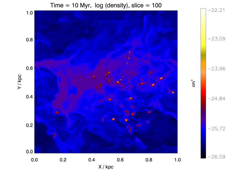
Figure 1: Left: Density slice through the $\mu$1T5 simulation at 10 Myr. Right: corresponding temperature histogram.

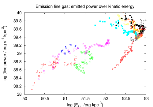
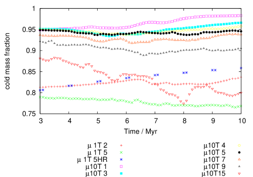
Figure 2: Left: Radiative power, emitted by the emission line gas (temperature in the range from 10,000 K to 20,000 K) over Kinetic energy of this gas. Different symbols are used for different runs shown at many times, as indicated in the legend. $\mu$xTy denotes an initial cloud density of x m_p cm^-3 and an initial temperature of the intermediate component of y Mio. K. Right: Cold gas ($T<10^{6}$ K) fraction over time.

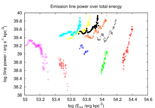
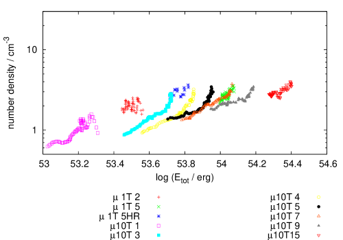
Figure 3: Left: Emission line power over total energy for different runs and simulation times. Right: Number density of the emission line gas over total energy.

3 Results

We show a density slice through run $\mu$1T5HR at the end of the simulation in Fig. 1. The cloud fragments can still be made out as the densest regions They are often embedded into the intermediate density gas. The temperature distribution for this timestep is shown in the same figure. The general trend is flatter than in 2D simulations. Still, we see a prominent peak at 14,000 K. There is also a significant accumulation at lower temperature, and around $10^{5}$ K. As in our previous 2D simulations, we ascribe the gas accumulated in the 14,000 K peak, and probably also in the $10^{5}$ bump to an equilibrium between shock heating and radiative cooling. In the following, we call all the gas with temperature in the range 10,000 K to 20,000 K the emission line gas.

An issue for such simulations is weather sufficient resolution was applied. In principle, the hydrodynamics equations do not include a dissipation scale for turbulence, which is artificially set by the numerical resolution. Also, the cool clumps would fragment further, if resolution would allow. However, the processes of interest may still be adequately represented, as is in fact usually the case for turbulence studies: The radiative cooling time of all gas below about $10^{6}$ K is much shorter than the simulation time. This gas is therefore constantly heated. The heating source is either shocks, or numerical heat conduction due to bad resolution of contact surfaces. In the first case, we would expect a correlation of the emission line power with the ambient temperature, in the second one a correlation with the kinetic energy. As Fig. 2 shows, the correlation with the kinetic energy is clearly the dominant one. The correlation, which most of the simulations follow with a spread of about one Dex, is linear. About $10^{12}$  erg are required for the emission of 1 erg/s in line emission. Interestingly, the two simulations with the highest external temperature follow a slightly offset pattern, emitting about a factor of ten less efficiently. The efficiency drop at high total energy can be seen more clearly in the plots of the emission line power versus total, and total kinetic energy (Fig.3). This confirms that we really simulate a realisation of the shock excitation scenario. The total energy drops monotonically with time, and hence the plots in Fig.3 May also be understood as an inverse time sequence. In general, the simulations follow a rather steep line, first, then levelling off to a flatter relation. The flatter tracks seem to form a kind of equilibrium line, whereas the steeper lines show that the systems evolve fast towards this equilibrium line.

Also shown in Fig. 2 is the fraction of gas colder than $10^{6}$ K against time. There is a dramatic difference between run $\mu$1T5 and $\mu$1T5HR, which is the same setup at double resolution. While the low resolution run shows a decline of the cold gas fraction, it increases in the high resolution one. Yet, for a given resolution, and initial cold gas fraction, there is a clear trend with the external temperature in the sense that at low external temperature, the cold gas fraction drops, whereas it rises at high external temperature.

4 Discussion

While, numerical resolution is an issue here, as always in turbulence simulations, the line power-kinetic energy correlation clearly shows that the dominant energy transfer is by shocks. The emitted power peaks near a kinetic energy density of $10^{54}$ erg/kpc³. Interestingly, some regions in the NLR of M51 (Bradley et al., 2004) are quite close to the correlation between the line power and the kinetic energy of the emission line gas, none are significantly below, and some are above, as expected if photo-ionisation comes on top of the shock excitation. High redshift extended emission line regions have a much higher kinetic energy density than considered here and emit less efficiently than indicated by the correlation. This may be hinted at by our highest energy simulations, but even higher kinetic energy density simulations are required to address this point.

The typical density in our emission line regions is too low (Fig.3), compared to observations, by a factor of about 100. This may be related to the quality of these simulations, but could also be a hint that the density in the sulfur line emitting regions, which is typically used for the density determination (e.g. Nesvadba et al., 2006), may not be typical for the majority of the emission line gas.

An ambient temperature of 5 Mio K is sufficient for turbulence enhanced gas cooling. Given the resolution limitations, higher temperatures might still work. Cosmologically, halo temperatures grow with time, and hence, this gives support to the idea that the external temperature may be a key factor to explain the absence of extended NLRs in low redshift radio galaxies.

References

- Antonuccio-Delogu & Silk (2008) Antonuccio-Delogu, V. & Silk, J. 2008, MNRAS, in press, ArXiv e-prints: 0806.4570
- Bradley et al. (2004) Bradley, L. D., Kaiser, M. E., & Baan, W. A. 2004, ApJ, 603, 463
- Dopita & Sutherland (1996) Dopita, M. A. & Sutherland, R. S. 1996, ApJS, 102, 161
- Krause & Alexander (2007) Krause, M. & Alexander, P. 2007, MNRAS, 376, 465
- Krause & Camenzind (2001) Krause, M. & Camenzind, M. 2001, A&A, 380, 789
- Mellema et al. (2002) Mellema, G., Kurk, J. D., & Röttgering, H. J. A. 2002, A&A, 395, L13
- Morganti et al. (2005) Morganti, R., Oosterloo, T. A., Tadhunter, C. N., van Moorsel, G., & Emonts, B. 2005, A&A, 439, 521
- Nesvadba et al. (2007) Nesvadba, N. P. H., Lehnert, M. D., De Breuck, C., Gilbert, A., & van Breugel, W. 2007, A&A, 475, 145
- Nesvadba et al. (2006) Nesvadba, N. P. H., Lehnert, M. D., Eisenhauer, F., et al. 2006, ApJ, 650, 693
- Smith et al. (2002) Smith, D. A., Wilson, A. S., Arnaud, K. A., Terashima, Y., & Young, A. J. 2002, ApJ, 565
- Sutherland et al. (2003) Sutherland, R. S., Bicknell, G. V., & Dopita, M. A. 2003, ApJ, 591, 238
- Ziegler & Yorke (1997) Ziegler, U. & Yorke, H. W. 1997, Computer Physics Communications, 101, 54