Quantum particle displacement by a moving localized potential trap

Abstract

We describe the dynamics of a bound state of an attractive $\delta$-well under displacement of the potential. Exact analytical results are presented for the suddenly moved potential. Since this is a quantum system, only a fraction of the initially confined wavefunction remains confined to the moving potential. However, it is shown that besides the probability to remain confined to the moving barrier and the probability to remain in the initial position, there is also a certain probability for the particle to move at double speed. A quasi-classical interpretation for this effect is suggested. The temporal and spectral dynamics of each one of the scenarios is investigated.

I Introduction

Recent developments in nanotechnology allow displacing miniscule particles, which can be as small as an atom. These particles’ relocation can be achieved either by optical tweezers tweezers or by Scanning Tunneling Microscopy (STM)STM . The STM moves an atom by creating a potential well at its vicinity. The atom is then trapped in the tip of the STM’s needle and can easily be relocated along with the tip’s position (see Fig.1). Beautiful structures with incredible (sub angstrom) accuracy were achieved STMgallery .

Since the atom is a quantum particle, localization at finite space is always partial. The sudden activation of the trapping well could cause an atom loss like in an equivalent decay process KM05 ; MG08 ; MugaWeiSnider . Moreover, in this paper we show that the sudden movement itself (not only the abrupt capturing) can be responsible for the atom escape. It is also shown that not only do some of the atoms remain (on the average) at their initial state, but some will move beyond the tip’s influence at double velocity.

Bound states subjected to sudden perturbations have been studied in relation to the so-called deuteron problem SM05 . The tunneling dynamics of a bound state has been reported in a time dependent well KM05 and after suddenly weakening the strength of the potential MG08 . Here we describe the transport of particles initially trapped in a well which is shifted at constant velocity along a waveguide. Under strong transverse confinement, the dynamics becomes effectively one-dimensional whenever all relevant energies are much smaller than the excitation quantum in the radial direction.

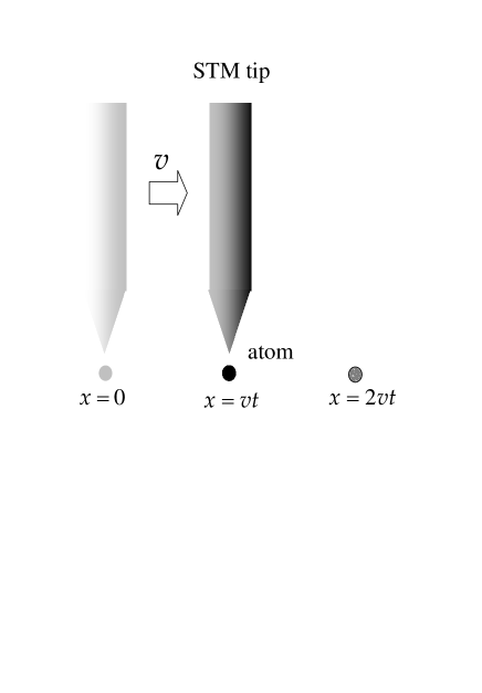
Figure 1: System schematic. A single atom displacement by an STM tip.

II The model

To simplify the system, the well is modelled by a one-dimensional delta function potential well. It should be stressed that a 1D negative(positive) delta potential is, in fact, an exponentially shallow potential well, and can model with great accuracy any well (barrier) whose physical dimensions are smaller than the de-Broglie wavelength of the particle Granot_11 .

Prior to $t=0$ the well is localized at $x=0$; however, for $t>0$ the well moves at constant velocity $v$. The potential well can then be formalized

$$V\left({x,t}\right)=\left\{{{\begin{array}[]{*{20}c}{-\gamma\delta\left(x\right)\hfill}&{\mbox{for}\hfill}&{t\leq 0\hfill}\\ {-\gamma\delta\left(x-vt\right)\hfill}&{\mbox{for}\hfill}&{t>0\hfill}\\ \end{array}}}\right.$$ (1)

Thus, the system dynamics are fully characterized by the Schrödinger equation:

$$i\frac{\partial\psi}{\partial t}=-\frac{\partial^{2}\psi}{\partial x^{2}}+V(x,t)\psi$$ (2)

where we adopted the units $\hbar=2m=1$.

The dynamics begin with the bound state of the $t<0$ potential, i.e.,

$$\psi(x,t=0)=\sqrt{\gamma/2}e^{-\gamma|x|/2}.$$ (3)

III Free evolution of the bound state

If it hadn’t been for the potential well, the particle’s probability density would spread out freely. If it is assumed that for $t>0$ the well is absent, and the Hamiltonian becomes purely kinetic, then for $t>0$ the dynamics is free, and it can be obtained using the superposition principle

$$\psi^{(\infty)}(x,t)=\int_{-\infty}^{\infty}dx^{\prime}{\rm K}_{0}(x,t|x,t^{\prime}=0)\psi(x^{\prime},t^{\prime}=0)$$ (4)

with the free propagator

$${\rm K}_{0}(x,t|x^{\prime},t^{\prime})=\bigg{[}\frac{1}{4\pi i(t-t^{\prime})}\bigg{]}^{\frac{1}{2}}e^{i\frac{(x-x^{\prime})^{2}}{4(t-t^{\prime})}}.$$ (5)

The time evolution of the initial bound state can be then simply written in terms of the Moshinsky function as

$$\psi_{0}(x,t) = \sqrt{\gamma/2}[M\left(x,-i\gamma/2,2t\right)+M\left(-x,-i\gamma/2,2t\right)].$$

where the Moshinsky function reads Moshinsky52 ; Moshinsky76 ; DMK08

$$M(x,k,{\rm t}):=\frac{e^{i\frac{x^{2}}{2{\rm t}}}}{2}w(-z),z=\frac{1+i}{2}\sqrt{{\rm t}}\left(k-\frac{x}{{\rm t}}\right)$$ (7)

in terms of the Faddeyeva function $w(z)$, which is defined as $w(z):=e^{-z^{2}}{\rm{erfc}}(-iz)$. On physical grounds it is clear that each of the $M$ functions corresponds to a freely time-evolved cut-off plane-wave. Such solution entails the well-known diffraction in time phenomenon, which consists of a set of oscillations in the density profile Moshinsky52 ; Moshinsky76 ; DMM07 . However, the imaginary wavector $-i\gamma/2$ makes such transients evanescent MB00 , leading to a uniform expansion.

IV Uniformly moving well

For $t>0$ the propagator should be extended to the $v\neq 0$ case, for which the corresponding propagator can be obtained using Duru’s method Duru89 and as well as by means of the path integral perturbation series Grosche93 . It can be conveniently written in terms of the free propagator and a perturbation term, represented by a Moshinsky function

$${\rm K}_{\delta}^{(v)}(x,t|x^{\prime},t^{\prime})={\rm K}_{0}(x,t|x^{\prime},t^{\prime})$$

$$+(\gamma/2)e^{i\frac{1}{2}\Big{[}v(x-vt)-v(x^{\prime}-vt^{\prime})+\frac{v^{2}(t-t^{\prime})}{2}\Big{]}}$$

$$\times M\left(|x-vt|+|x^{\prime}-vt^{\prime}|,+i\gamma/2,{\rm t}\right)$$ (8)

Figure 2: Transients developed in the density profile of a bound state $|\psi(x,t)|^{2}$, for a moving delta with $v=1.5$ and $\gamma=0.7$. The dotted line follows the trajectory of the well $x=vt$, while the dashed line corresponds to $2vt$. Units $\hbar=2m=1$ are used in all figures.

The time evolution of the state in Eq. (3) can be also obtained in close-form, using the integral EK88

$$\int_{-\infty}^{0}dx^{\prime}e^{ikx^{\prime}}M(|x^{\prime}|+|x^{\prime}|,-iV_{0},t)$$ (9)

$$= \frac{1}{V_{0}-ik}[M(|x|,k,t)-M(|x|,-iV_{0},t)].$$

Taking $t^{\prime}=0$ and using Eqs. (3), (IV) and (9), one can readily find

$$\psi_{\delta}^{(v)}(x,t)=\psi_{0}(x,t)$$

$$-e^{ivx/2-i\frac{v^{2}t}{4}}\frac{(\gamma/2)^{\frac{3}{2}}}{\gamma-iv/2}$$

$$\times\big{[}M(|x-vt|,-v/2-i\gamma/2,2t)-M(|x-vt|,i\gamma/2,2t)\big{]}$$

$$-e^{ivx/2-i\frac{v^{2}t}{4}}\frac{(\gamma/2)^{\frac{3}{2}}}{\gamma+iv/2}$$

$$\times\big{[}M(|x-vt|,v/2-i\gamma/2,2t)-M(|x-vt|,i\gamma/2,2t)\big{]},$$

as the sum of a free term plus a perturbation.

The adiabatic Massey parameter EK88 , which distinguishes the distinct dynamical regimes is therefore

$$\theta\equiv\frac{v}{\gamma},$$ (11)

so that for $\theta\ll 1$ the adiabatic dynamics is recovered while $\theta\gg 1$ corresponds to the infinitely fast displacement of the well (free evolution).

Indeed, the eigenstate of a moving delta well is Duru89

$$\psi_{b}^{(v)}(x,t)=\sqrt{\gamma/2}e^{i\frac{\gamma^{2}-v^{2}}{4}t}e^{ivx/2}e^{-\gamma|x-vt|/2},$$ (12)

which for $t=0$, becomes $e^{ivx/2}\psi(x,0)$. The fraction that remains bounded for $t\rightarrow\infty$ is

$$|\langle\psi_{b}^{(v)}(0)|\psi(0)\rangle|^{2}=\frac{\gamma^{4}}{(\gamma^{2}+v^{2})^{2}}=\frac{16}{(4+\theta^{2})^{2}},$$ (13)

for $v\gamma\ll 1$, the exponential becomes $e^{ivx/2}\sim 1$ in the spatial range of the initial bound state, and the overlap becomes unity.

V Three scenarios

When $t\rightarrow\infty$ the three domains that were discussed at the introduction (the particles that remain at the vicinity of $x=0$, the ones that are localized to the well at uniform velocity and the ones that propagate at double velocity) eventually appear. The wavefunction can be written as a supperposition of three terms:

$$\psi\sim\psi_{free}+\psi_{well}+\psi_{2v}.$$ (14)

where

$$\psi_{free}(x,t) \cong \sqrt{\frac{2}{i\pi\gamma t}}e^{i\frac{x^{2}}{4t}}\frac{1}{1+(x/\gamma t)^{2}},$$

$$\psi_{well}(x,t) \cong \frac{\sqrt{\gamma/2}}{1+(v/2\gamma)^{2}}e^{i\frac{v}{2}x+i\frac{(\gamma^{2}-2v^{2})t}{4}-\frac{\gamma}{2}|x-vt|},$$

$$\psi_{2v}(x,t) \cong \frac{1}{1+iv/2\gamma}\frac{\sqrt{it\gamma/8\pi}}{(x-2vt)+i\gamma t}e^{i\frac{x^{2}}{4t}-iv^{2}t}.$$

The first term $\psi_{free}$ describes the free evolution of the initial state in the absence of the well, as can be appreciated from the structure of the propagator. The second contribution remains localized in the moving trap and follows its classical trajectory $x=vt$, while the last term is responsible for the appearance of a peak in the density profile at $x=2vt$. This contribution results from the partial reflection from the attractive well of the initial state probability density located at $x>vt$.

Since in the initial state, the particle was localized in a region as small as $\Delta x\sim\gamma^{-1}$ the uncertainty in the particle’s velocity behave like $\Delta v\sim\gamma$ and therefore, as can be seen in Eq. 14, the spatial width of the two peaks $0$ and $2v$ gets wider approximately like $\Delta x\sim\gamma t$ (unlike the width of the localized part, which remains $\sim\gamma^{-1}$). Therefore, the distinction between the three parts can appear only when $v>\gamma$ (or $\theta>1$). Moreover, due to their initial width, the peaks shape appears only when $t\gg(v\gamma)^{-1}$.

The probability density of the exact solution with a comparison to the approximation, which focuses on the three terms is illustrated in Fig.3.

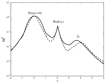
Figure 3: Spatial distribution of the probability density $|\psi|^{2}$ (solid line) and its approximation (dashed line). The three domains ($v=0$,$v$, and $2v$) are marked. The parameters are $\gamma=10$, $v=40$ and $t=0.05$.

VI Asymptotics

The transition from the initial stationary bound state to the final moving one involves the two natural frequencies of the system: The frequency (energy) of the initial state $f_{1}=\gamma^{2}/8\pi$ and the kinetic energy of the moving particle $f_{2}=v^{2}/8\pi$. The $x=0$ and the $x=2vt$ peaks are affected only by the frequency $f_{2}$, however, the $x=vt$ one oscillates with three harmonics $f_{1}$, $f_{2}-f_{1}$ and $2f_{2}-f_{1}$. In Fig.4 the temporal dynamics of the three peaks is shown. The $x=0$ and the $x=2vt$ decay like $\sim t^{-1/2}$, while the $x=vt$ one converges to its final constant value

$$|\psi(x=vt,t\rightarrow\infty)|^{2}=\frac{\gamma/2}{(1+(v/2\gamma)^{2})^{2}}.$$ (16)

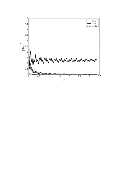
Figure 4: The temporal dynamics of the three peaks ($x=0$, $x=vt$ and $x=2vt$). The system’s parameters are: $\gamma=10$, $v=20$.

In Fig. 5 a numerical spectral distribution $\Psi(f)\equiv FFT[|\psi|^{2}]$ (FFT stands for the Fast Fourier Transform) of each one of the peaks is presented. The four different frequencies are clearly shown.

The ’A’ peak corresponds to the frequency $f_{1}=\gamma^{2}/8\pi$. The ’D’ and ’E’ peaks correspond to the frequency $f_{2}=v^{2}/8\pi$, the ’B’ one stands for $f_{3}=|f_{2}-f_{1}|=|v^{2}-\gamma^{2}|/8\pi$ and finally ’C’ stands for $f_{4}=f_{3}+f_{2}=|2v^{2}-\gamma^{2}|/8\pi$.

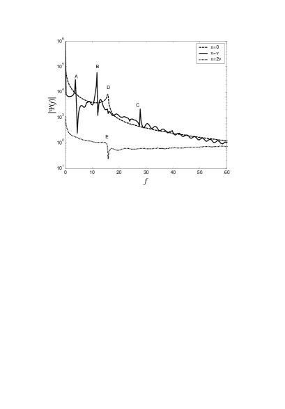
Figure 5: The spectral distribution $\Psi(f)$ of the three peaks (of Fig.4).

VII Semi-classical realization

Clearly, the double velocity effect cannot be classical, since a localized state will remain localized in the classical world. However, the origin of this effect has partially a classical interpretation. Quantum mechanically, the particle in the initial state is not completely localized inside the well. In fact, when the well is very narrow most of the chance is to find the localized particle outside the well.

It is also instructive to investigate the system in a moving frame of reference, in which the well is at rest (originally, at the lab reference the well moves to the right).

At $t=0$ the particle (at the well’s reference frame) begins to move to the left with respect to the well. We can regard it as three different scenarios: particle at the right of the well (gray) at the well (black) at its left (white) At $t=0$ all three types begin to moves simultaneously to the left at velocity $v$ (Fig.6A).

The white is free - so it remains at velocity v to the left. The black is trapped - so its average velocity is zero. But the gray hits the barrier and turns back with velocity $-v$, i.e., the final scenario is shown at Fig.6B.

When we return to the lab frame of reference (where the well moves to the right), we see that the white one didn’t move, the black moved with the well at velocity $v$ and the gray moved with velocity $2v$ (Fig.6C).

Obviously, this semiclassical interpretation is possible only due to the partial localization, which is a manifestation of Quantum mechanics.

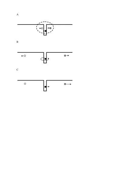
Figure 6: Semiclassical realization of the three domains.

VIII Conclusion and Discussion

We have presented a 1D quantum model for an atom displacement with an STM tip. The model consists of a delta function well, which model the STM’s potential at the vicinity of its tip end, which moves uniformly. It was shown that the probability to remain trapped in the moving tip is $\frac{\gamma^{4}}{(\gamma^{2}+v^{2})^{2}}=\frac{16}{(4+\theta^{2})^{2}}$.

Moreover, it was shown that besides the trapped particles, and the particles that remain close to their initial state, there is also a third group of particles, which propagates at double velocity ($2v$) away from their initial position. We show that the probability for each one of the three groups has a different temporal dynamics.

- (1) Jeffrey R. Moffitt, Yann R. Chemla, Steven B. Smith and Carlos Bustamante,”Recent Advances in Optical Tweezers”, Annual Review of Biochemistry, 77, 205-228 (2008).
- (2) G. Binnig and H. Rohrer, ”Scanning Tunneling Microscopy–from Birth to Adolescence,” Rev. Mod. Phys. 59, 615 (1987).
- (3) http://www.almaden.ibm.com/vis/stm
- (4) T. Kramer and M. Moshinsky, J. Phys. A: Math. Gen. 38, 5993 (2005).
- (5) J.G. Muga, G.W. Wei, and R.F. Snider, Annal. Phys. , 252, 336-356 (1996)
- (6) A. Marchewka and E. Granot, arXiv:0804.3317.
- (7) M. Moshinsky and E. Sadurní, SIGMA 1, 003, (2005).
- (8) E. Granot, Phys. Rev. B 71, 035407 (2005)
- (9) M. Moshinsky, Phys. Rev. 88, 625 (1952).
- (10) M. Moshinsky, Am. Jour. Phys. 44, 1037 (1976).
- (11) A. del Campo, J. G. Muga, M. Kleber, Phys. Rev. A, 77, 013608 (2008).
- (12) A. del Campo, J. G. Muga, and M. Moshinsky, J. Phys. B 40, 975 (2007).
- (13) J. G. Muga and M. Büttiker, Phys. Rev. A, 62, 023808 (2000).
- (14) I. H. Duru, J. Phys. A: Math. Gen. 22, 4827 (1989).
- (15) C. Grosche, Ann. Phys. 6, 557 (1993).
- (16) W. Elberfeld and M. Kleber, Am. J. Phys. 56, 154 (1988).